Article

Turbulent Flow Fields Over a 3D Hill Covered by Vegetation Canopy Through Large Eddy Simulations

1
School of Civil Engineering & Mechanics, Huazhong University of Science and Technology, Wuhan 430074, China
2
Department of Architecture and Building Engineering, Tokyo Institute of Technology, Yokohama, Kanagawa 1528550, Japan
*
Author to whom correspondence should be addressed.
Energies 2019, 12(19), 3624; https://doi.org/10.3390/en12193624
Submission received: 14 August 2019 / Revised: 16 September 2019 / Accepted: 16 September 2019 / Published: 23 September 2019
(This article belongs to the Special Issue Engineering Fluid Dynamics 2019-2020)

Abstract

:
The flow fields over a simplified 3D hill covered by vegetation have been examined by many researchers. However, there is scarce research giving the three-dimensional characteristics of the flow fields over a rough 3D hill. In this study, large eddy simulations were performed to examine the coherent turbulence structures of the flow fields over a vegetation-covered 3D hill. The numerical simulations were validated by the comparison with the wind-tunnel experiments. Besides, the flow fields were systematically investigated, including the examinations of the mean velocities and root means square of the fluctuating velocities. The distributions of the parameters are shown in a three-dimensional way, i.e., plotting the parameters on a series of spanwise slices. Some noteworthy three-dimensional features were found, and the mechanisms were further revealed by assessing the turbulence kinetic energy budget and the spectrum energy. Subsequently, the instantaneous flow fields were illustrated, from which the coherent turbulence structures were clearly identified. Ejection-sweep motion was intensified just behind the hill crest, leading to a spanwise rotation. A group of vertical rotations were generated by the shedding of the vortex from the lateral sides of the hill.

1. Introduction

As we all know, turbulence has a very important research position in many fields, and the turbulent flow field on the topography in different fields is closely watched by many researchers, including the wind turbine sittings [1], the pollution diffusions [2], estimation of aerodynamic loadings on structures [3], identifications of the tree damage with high risk [4], as well as the forest fire propagation [5]. Given the complexity of the flow over real complex topographies, many studies have been conducted to clarify the turbulent boundary layer (TBL) flow over simplified hills. The relevant research is primarily about the smooth topographies. Very little research is about the flow over topographies with the canopy covered, which can be divided into three groups, i.e., the flat topography, the 2D ridge, and the 3D hill.
Dupont and Brunet examined the coherent structures in canopy edge flow over flat terrain by large eddy simulations (LES) [6]. In their research, the development of turbulent structures was revealed, and we can see from the schematic that many of them are strikingly similar to the development of coherent structures observed in mixed layers. Takahashi et al. investigated the turbulence characteristics of the flow over a 2D ridge with a rough surface in wind tunnel experiments [7] and the effects of roughness density were studied. It was found that the mean velocity profiles were not sensitive to the density of the roughness and the roughness served as strong windbreaks, weakening the wind velocity near the hill surface. Cao and Tamura experimentally studied the roughness effects on TBL flow over a 2D ridge [8], in which above the top of the rough hill the acceleration ratio was slightly larger than the smooth hill and because the separation bubble extends to the downstream of the hill, the reattachment length was also larger than the smooth hill. Subsequently, Cao and Tamura further examined the effects of ground roughness on the flow over a 2D ridge with or without sudden roughness change [9]. In their research, four situations were considered, i.e., (i) smooth hill in smooth flow, (ii) rough hill in rough flow, (iii) smooth hill in rough flow, and (iv) rough hill in smooth flow. It was concluded that the velocity deficit varied with roughness conditions on the hill surface or inflow area, thereby creating a completely different turbulence structure. Dupont et al. studied the turbulent flow over a 2D ridge with a vegetation canopy cover using LES [10], in which the coherent structures were identified. According to their research, the turbulence in the wake region is mainly caused by the superposition of the following three turbulent structures: (i) the large turbulent structure caused by the high shear layer, (ii) a turbulent structure caused by a back pressure gradient caused on the back of the ridge, and (iii) a turbulent structure due to the presence of the canopy. Ishihara et al. conducted a study of the flow over a 2D ridge and a 3D hill under smooth and rough ground by wind tunnel experiment [11]. Detailed information was provided, covering the inflow condition, the mean, as well as the fluctuating velocities. Afterwards, Ishihara and Hibi examined the flow over a rough 3D hill by Reynolds-averaged Navier–Stokes (RANS) models [12]. Standard k-ε model and Shin’s nonlinear model were tested and the performance of Shin’s nonlinear model was found to be much better than k-ε model. Tamura et al. adopted LES to reproduce the experimental data by Ishihara et al. [11,13], and the LES results were consistent with the experiments both for the smooth and rough hills. Most recently, Liu et al. numerically studied the flow over a blocks-covered flat ground [14], a vegetation-covered flat ground, a vegetation-covered 3-D hill, as well as a real forest-covered terrain. The method yielding the turbulent inflow, determining the grid spacing, and the settings of LES were validated.
However, most of the studies on the flow over a rough 3D hill only provided the flow information on the symmetry plane. There has been scarce research giving the 3D characteristics of the flow over a rough 3D hill. Therefore, systematic information of the 3D flow fields will be provided in the present study. The representative parameters, i.e., the mean velocities and root means square (r.m.s.) of the velocity fluctuations were examined. Furthermore, the three-dimensional features and the mechanisms were revealed by investigating the turbulence kinetic energy (TKE) budget and the spectrum energy.

2. Numerical Model

2.1. Governing Equations

Time-dependent Navier-Stokes (N-S) equations of large eddy simulations in Cartesian coordinates (x, y, z) are:
ρ u ˜ i x i =   0 ,  
ρ u ˜ i t + ρ u ˜ i u ˜ j x j   =   x j ( μ u ˜ i x j ) p ˜ x i τ ˜ i j x j ,  
where p ˜ and u ˜ i represent the filtered pressure and velocities, respectively, ρ denotes the density, μ denotes the viscosity, and τ ˜ i j is the sub-grid scale (SGS) stress. To close the equations for the filtered velocities, a model for τ ˜ i j is required:
τ ˜ i j   =   2 μ t S ˜ i j + 1 3 τ ˜ k k δ i j ,
S ˜ i j   =   1 2 ( u ˜ i x j + u ˜ j x i ) ,
where S ˜ i j denotes the rate-of-strain tensor, μ t is the SGS turbulent viscosity, and δ i j is the Kronecker delta. The Smagorinsky–Lilly model is used to determine the SGS turbulent viscosity [15]:
μ t = ρ L s 2 | S ˜ | =   ρ L s 2 2 S ˜ i j S ˜ i j ,
L s = min ( κ d ,   C s V 1 / 3 ) ,
where L s is the mixing length, κ is the von Kármán constant (0.42), d is the distance to the wall, and V is the cell volume. Here, Cs is set as 0.1 according to Iizuka and Kondo [16].
When the cells are in the viscous sublayer, the shear stresses are yielded from:
u ˜ u ˜ τ   =   ρ u ˜ τ y μ .
Accurately modeling the inflow is essential for the success of simulating the flow in the 3D hill wake. In the present study, the upstream blocks arrangement in the simulations were identical to those in the experiments by Ishihara et al. [12]. Besides this, the distance between the roughness blocks to the location where the 3D hills were placed was also set identically to that in the wind tunnel experiment. The additional drag force is used to simulate the roughness elements:
ρ u ˜ i t   +   ρ u ˜ i u ˜ j x j   =   x j ( μ u ˜ i x j )     p ˜ x i     τ ˜ i j x j   +   f ˜ u , i ,
where the drag force term f ˜ u , i = CdAf ρ u ˜ i | u ˜ |, Af is the frontal area of the roughness blocks, Cd = 100 to model the large drag effects in the solid roughness blocks, consistent with the method by Lee and Sung [17]. The geometry of the computational domain and the grid system can be used from the previous work, ignoring the effects of different rough block layouts, which saves manpower and material resources and, according to the relevant experimental theory, only the function that determines geometry of the rough block needs to be modified.
To model the canopy, the drag force term, f ˜ u , i , is substituted in the momentum equations in the same form as Equation (8). The drag force term is determined by f ˜ u , i = Cd Af ρ u ˜ i | u ˜ |, where Cd = 0.2 denotes the drag force coefficient, Af = 0.6 m−1 is the leaf-area density, |u| is the velocity magnitude. Cd and Af are determined according to the study by Ishihara and Qi [18].

2.2. Configurations

Before providing the detailed configurations of the computational model, the wind tunnel experiments by Ishihara et al. should be briefly introduced, which is the case the present LES aimed to reproduce [11]. During the experiment, a neutral layered atmospheric boundary layer (ABL) was simulated by two 60 mm high cube arrays followed by 20 m and 10 mm high cubes, covered on the 1.2 m test section. The rough element was covered with an artificial turf with a height of 5 mm and the rest of the floor of the test building was 5.8 m long. At the contraction exit, the mean wind speed   U i n   =   5.4   m   s 1 . The boundary layer thickness, δ , was nearly 0.36 m at the hill center, and the scale, λ, was about 1:1000 of the ABL, based on the power spectra of the longitudinal velocity component. The wind speed outside the boundary layer was measured as U   =   5.8   m   s 1 . As a result, the simulated boundary layer had a bulk Reynolds number,   R e b = U δ / ν   =   1.4   ×   10 5 , and the friction Reynolds number R e τ   =   U τ z 0   /   ν   =   6.4 , where,   U τ =     τ   /   ρ   = 0.32 m s−1, τ is the shear stress in an arbitrary layer, z 0 = 0.3 mm refers to the roughness height determined by comparing the resulted mean streamwise velocity profile based on the logarithmic law: U (z) =   U τ κ   ln   z z 0   .
The computational domain is shown in Figure 1. The origin point (0, 0, 0) was 3.4 m downstream from the roughness blocks. The 3D hill was placed at the origin point, exhibiting a shape: z s ( x ,   y )   =   h   cos 2 π ( x 2   +   y 2 ) 1 / 2 / 2 L when ( x 2   +   y 2 ) 1 / 2   <   L , and z s ( x ,   y )   =   0 when ( x 2   +   y 2 ) 1 / 2   >   L , where h = 40 mm and L = 100 mm. z = zzs (x, y), was employed to determine the height above the ground. A domain size in spanwise direction of approximately Ly = 1.8 δ was adopted. Ly = 1.8 δ was further confirmed to be enough, since the two-point correlations converged to zero in the half-width of Ly. As for the necking zone, in the upstream region, a buffer zone (i.e., 2.0 m long, 5.6 δ ) was used to absorb upward-propagating wave disturbances. Vertical domain size was the same as that in the wind tunnel, Lz = 2.5 δ . The outlet was set at 6.7 δ downstream from the origin point (0, 0, 0). A grid nesting procedure was adopted. Two nested grid domains (coarse and fine) were adopted, as shown by the red dashed lines in Figure 1. The fine grid domain covered a range of (Lx′, Ly′, Lz′) = (12L, 2L, 3L).

2.3. Mesh of the Model

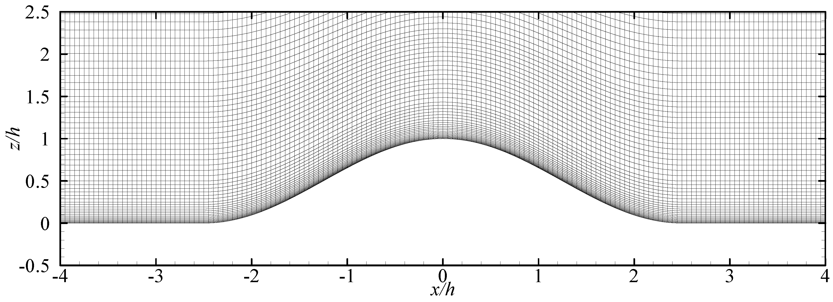
For the grid size, in the vertical direction, the grid was stretched starting with a vertical grid spacing of 0.2 mm on the surface in both the fine and coarse grid domains. The resulting vertical grid resolution on the surface z +   =   U τ Δ z min   /   ν < 1.0 covered most of the domain, except for the windward part of the hill where the maximum z + was less than 2. The vertical grid should be also sufficiently fine enough to capture the turbulent flow fields induced by the large wind shear, which was located at the height of about h. The vertical size of the wind shear-induced eddies is proportional to the shear length-scale Ls = U(z)/[dU(z)/dz], where U denotes the mean streamwise velocity. From a pre-modeling of the case with Δ z = 10 mm in the shear layer region, Ls was found to be nearly 8 mm. In the present LES, Δ z was finally set to be 4 mm at z = 80 mm. In the region z < 80 mm, the vertical grid was increased by a hyperbolic function. Exceedingly large aspect ratios ( Δ x / Δ z ,   Δ y / Δ z ) may cause numerical errors in the horizontal direction and some distortions of the eddies. The value of 10 was adopted in the present LES. Given Δ z min   =   0.2   mm , Δ x and Δ y in the fine grid domain should be about 2 mm. Moreover, in the grid independence examinations, the models with Δ x y = 5.65, 4.0, 2.8, and 2.0 mm were calculated. The meshes Δ x y = 2.8 and 2.0 mm gave roughly the same results, suggesting the grid-independent results were achieved. From this result, we got a more convincing conclusion, that is, in the LES of the current research field, the aspect ratio can very well estimate the actual situation of the turbulent structure on the 3D hill. Thus, a grid size 2.0 mm in horizontal direction was applied in the fine grid region. Finally, the corresponding nondimensional grid resolutions of fine domain in x, y, and z directions were x + = [3.2, 23], y + = [3.2, 23], z + = [0.23, 1.9]. Downstream of the fine grid domain and upstream of the roughness blocks, Δ x was stretched at a ratio of 1.2. Total grid number was 2.6 × 10⁷. The vertical slice showing the grid distribution is provided in Figure 2. The mean skin friction coefficient was determined as:
C f   =   τ w 1 2 ρ U h 2
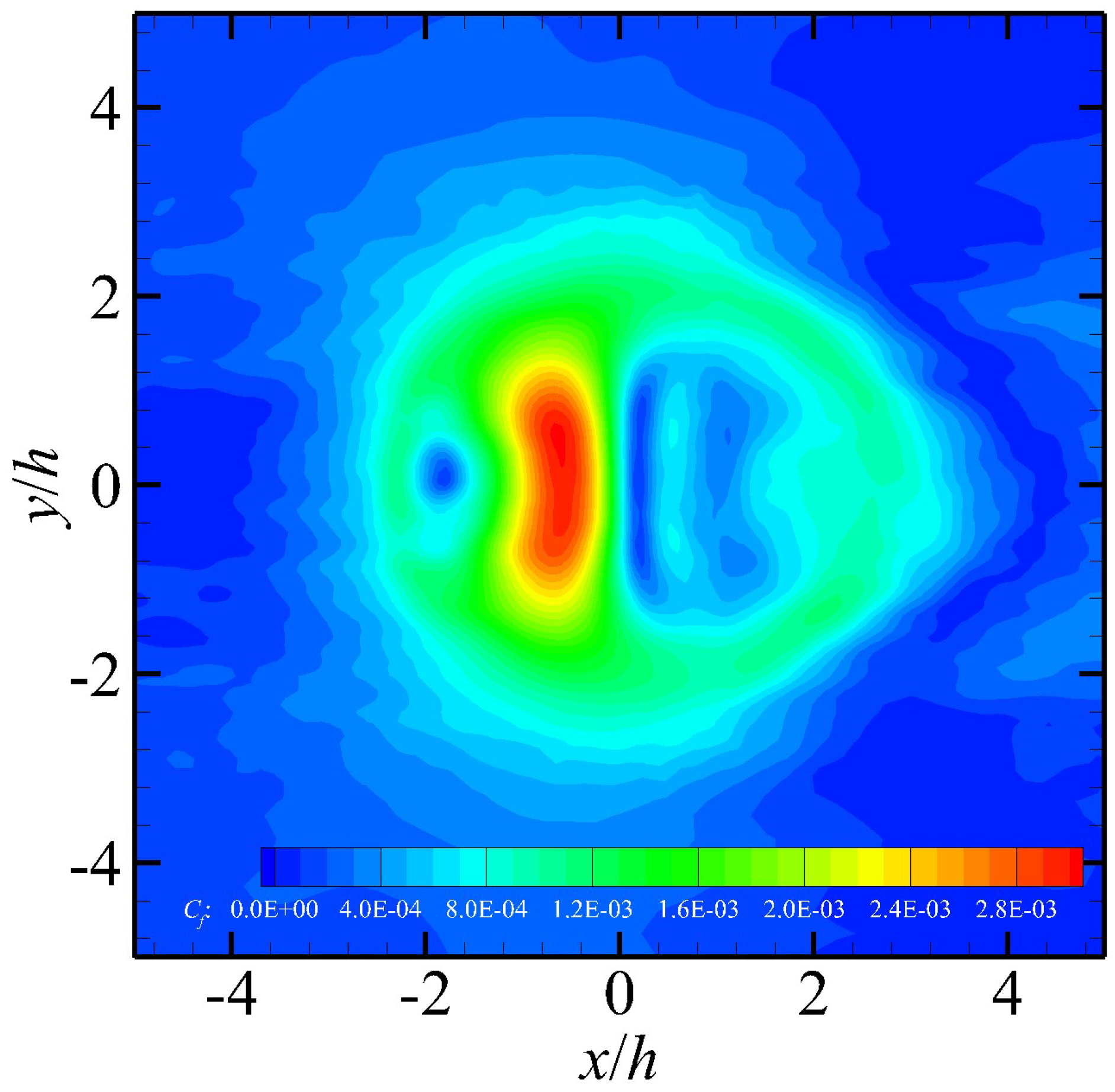
where, τ w is the mean shear stress on the wall, as shown in Figure 3, where it is clear that the maximum Cf is located at the front side of the hill reaching to about 0.003.

2.4. Boundary Conditions

A stress-free condition was used at the top and the spanwise sides. Uniform wind flow with a 5.4 m s−1 was set at the inlet. The gradient-free boundary condition was set at the outlet. The no-slip condition was applied at the bottom. The stress-free condition at the top and the symmetry condition at the lateral sides were different than the no-slip condition in the wind tunnel. However, considering the very thin TBL at those smooth walls in the wind tunnel (at a scale of 10−3 m) and the fact that the induced turbulence at the walls are far from the region of interest, these boundary condition differences are supposed to have negligible effects on the LES solutions. By validating the numerical model, artificially changing the boundary conditions in wind tunnel to those adopted in the present LES was proven to be satisfactory.

2.5. Solution Schemes

Finite volume method (FVM) was applied in LES. For the convection and viscous terms in the LES method, the second-order center difference format was used for calculation, while for the viscous terms, the second-order implicit format was used for processing. Time step size Δt was set as 0.0001 s and in convective time units, Δt* = ΔtUh/h = 0.01, where Uh = 3.9 m s−1 is the mean velocity at the point (x = 0, y = 0, z = h) in the absence of the 3D hill. The Courant–Friedrichs–Lewy (CFL) number is based on the time step size (Δt), velocity (ui), and grid size (Δxi), expressed as C = ΔtΣuixi. It is worth noting that the CFL number is limited to no more than 2 (i.e., Cmax = 0.9) throughout the computational domain. For solving discrete equations, it is possible to use the SIMPLE (semi-implicit pressure linked equations) algorithm, which is very effective and popular. Due to the huge amount of computation, the entire calculation process needs to be performed on a high performance 3PCs in parallel. The simulation process takes 435 hours to complete, but after simulating nearly 400 time units, it was found that the initial transient effects disappeared. Statistical convergence was achieved when | u i y     u i + y /   ( u i y   +   u i + y ) / 2 |   <   1 % in the near wake of the 3D hill, which was over 350 time units, where   denotes the time-averaging process.
Quantifying the relative importance of the SGS viscosity υ s g s is important for determining whether only the resolved fluctuations are sufficient for the statistics. The equivalent eddy-viscosity υ e , evaluated as υ e =   2 3 k δ i j     u i u j /   2 S i j , where k =   1 2 u i u i , u i is the deviation from u i , and the norm   of a matrix ϕij denotes ( ϕ i j ϕ i j ) 1 / 2 , can be adopted to examine the relative importance between the resolved fluctuations and the modeled ones using the SGS model. In the present LES, υ e / υ s g s in the 3D hill wake was found to be less than 5%, indicating that the effects of the SGS model on the present resolved LES results were negligible. As a result, only the resolved eddies in the present LES were considered for the statistics.

3. Numerical Results

3.1. Generated TBL

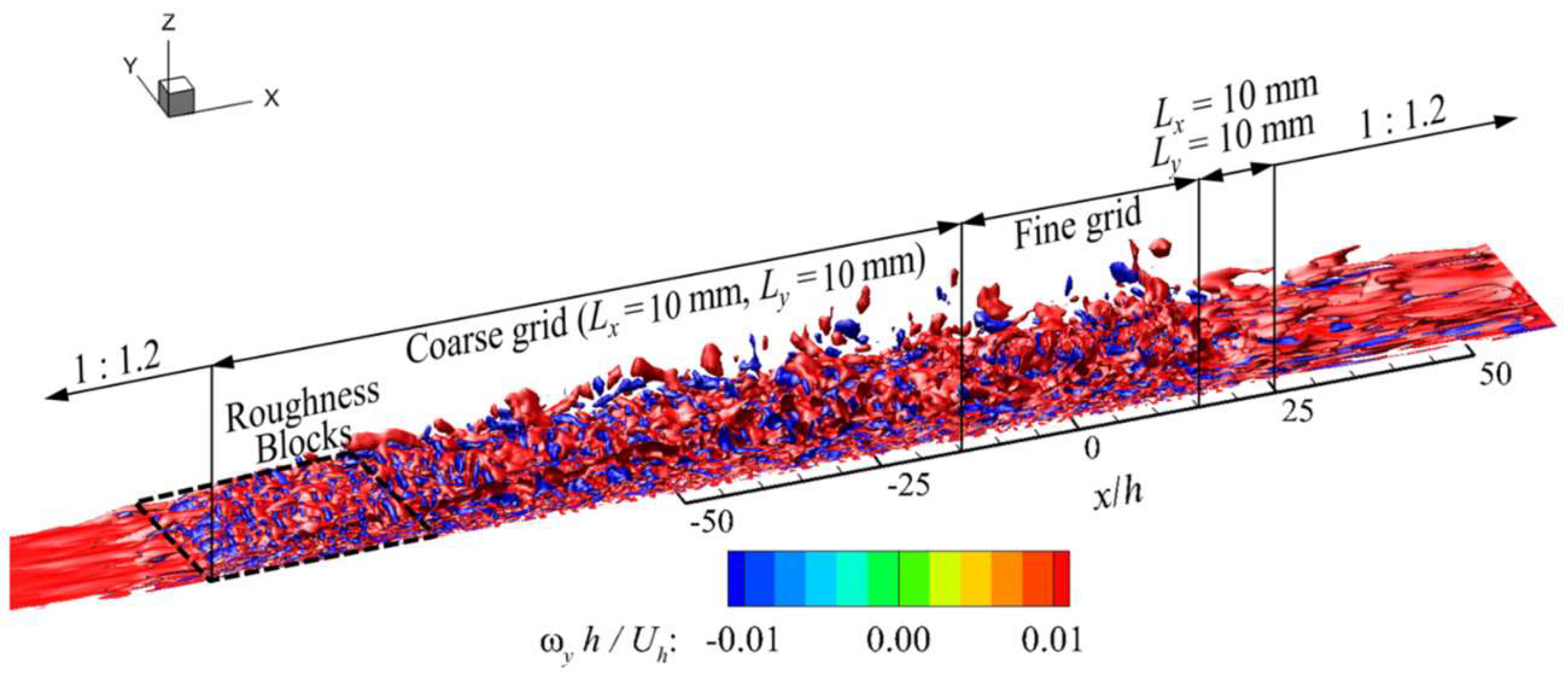
The profiles of incoming TBL, both in terms of u and r.m.s. of fluctuating velocities, σ u i , are critical for a precise reproduction of 3D hill wake flow, playing significant roles in the separation and reattachment, and in return affecting the coherent turbulence structures. Thus, before the detailed discussions of the turbulence properties in the wakes of the 3D hill, it is worthwhile to examine the performance of the adopted incoming TBL generation method. Firstly, it is noteworthy to get an insight of the instantaneous turbulent flow fields before the presentation of the flow fields statistics. Figure 4 displays a snapshot of two iso-surfaces of spanwise vorticity ωy = w / x     u / z = −15 s−1 and 15 s−1 of the TBL in the absence of 3D hills at 400 time units. As soon as the flow travels downstream to the roughness block region, strong coherent turbulence structures are induced. Further propagating downstream, the flow experiences an obvious boundary-layer growth, together with which, the streak structures are enhanced; on the contrary, the ejection-sweep motions are shredded.
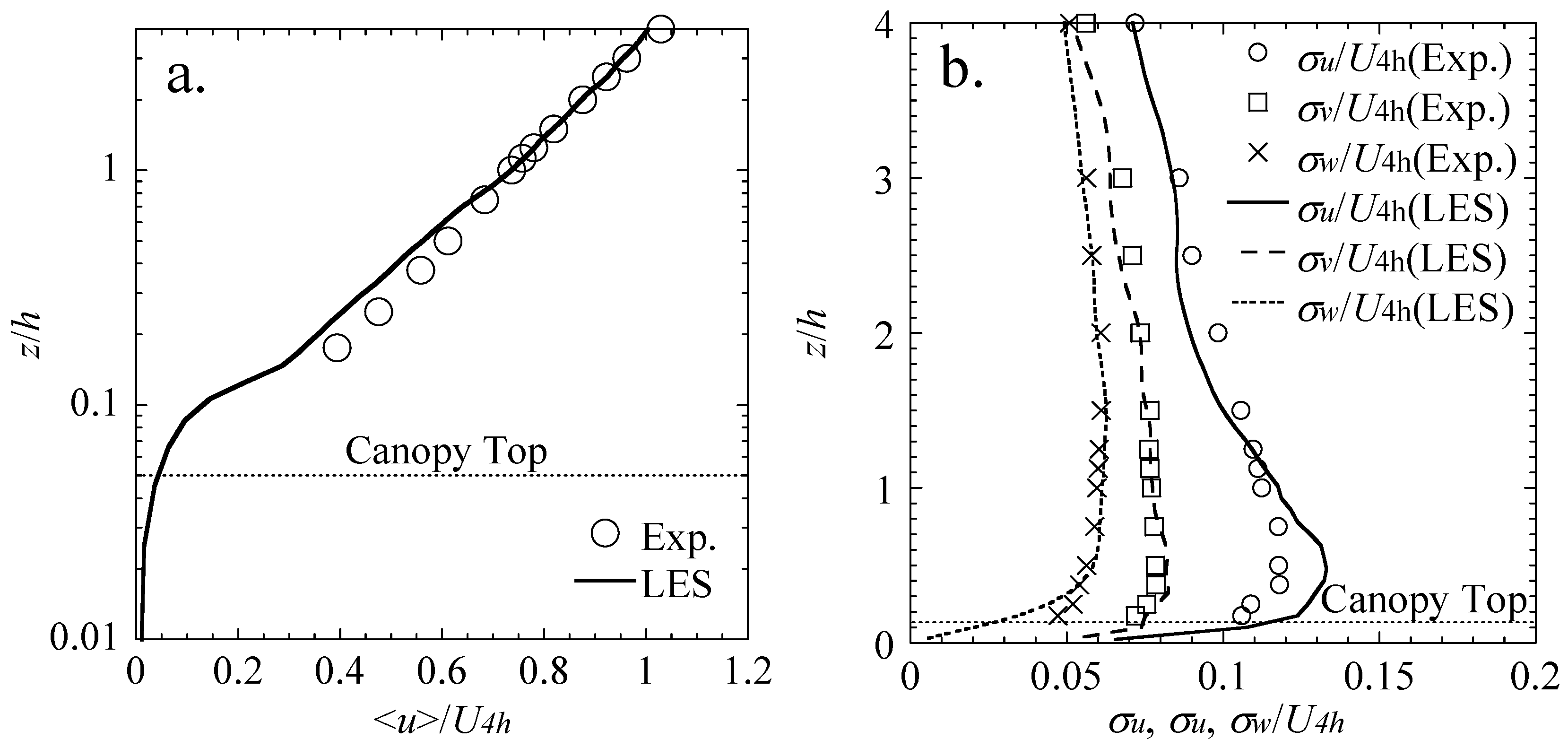
After the flow reached an equilibrium state (400 time units), statistics of u and σ u i were collected over 400 time units. In addition, assuming statistics in spanwise direction is homogeneous, the profiles of u and σ u i are further smoothed by averaging them over all y     ( 0.5 L ,   0.5 L ) locations at each (0, z) position. The resulted profiles of u and σ u i , as well as the comparison with those in the experiment by Ishihara et al. [11], are shown in Figure 5, where the normalization, using h and U4h, which is the same as the experiment, is performed. U4h = 5.3 m s−1 in the present LES and 5.2 m s−1 in the wind tunnel experiment. The comparisons show good agreement.

3.2. Instanteneous Flow Fields

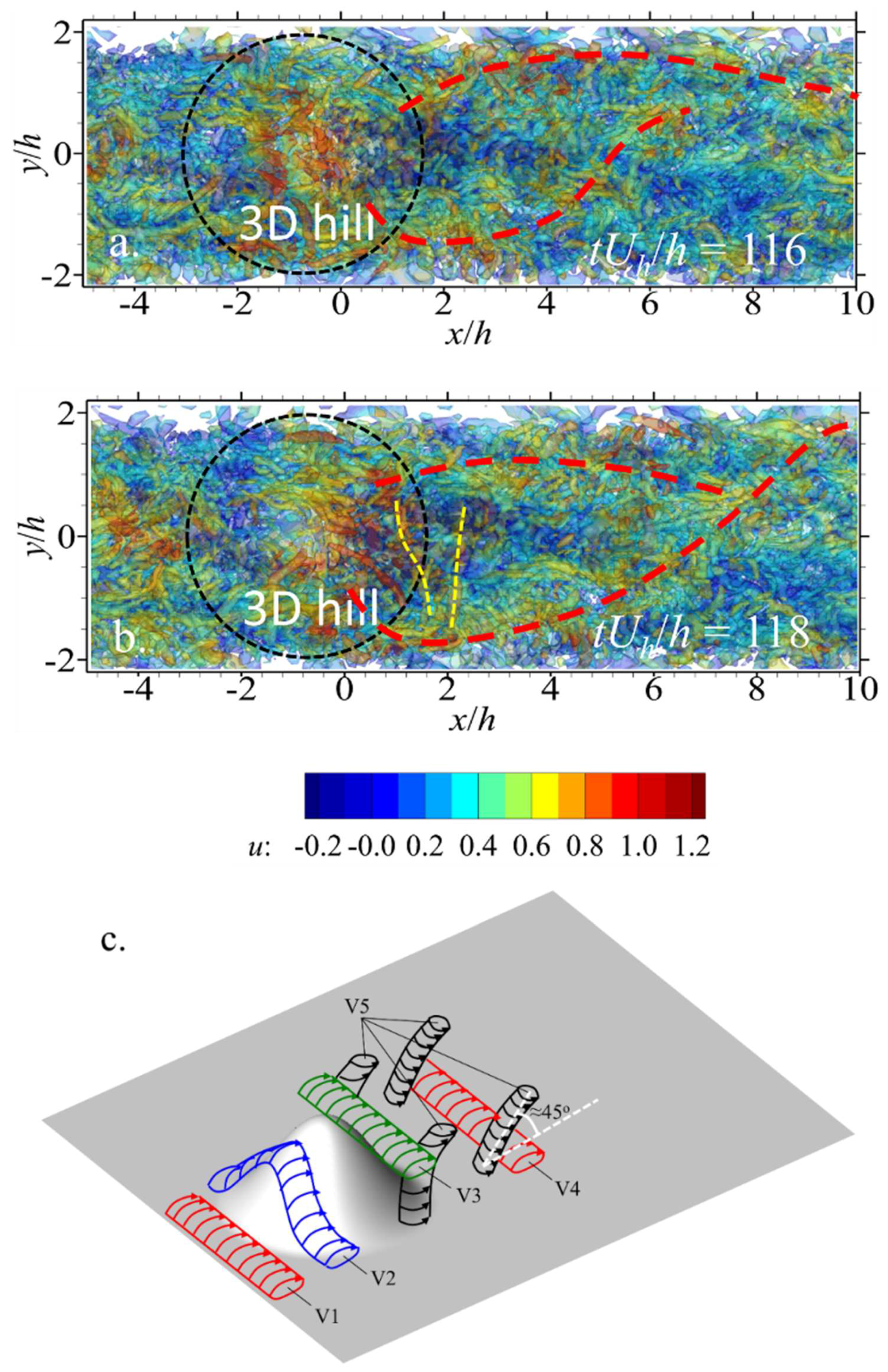
The Q-criterion was adopted to clarify the instantaneous turbulent structures, Q   =   1 / 2 ( S i j S i j     Ω i j Ω i j ) , where S i j   =   1 / 2 (   u ˜ i / x j       u ˜ j / x i ) and Ω i j = 1 / 2 (   u ˜ i / x j +   u ˜ j / x i ) , respectively. The snapshots of iso-surfaces of the normalized Q equaling to 3.0 and −3.0 at tUh/h = 116 and 118 are plotted in Figure 6.
The iso-surfaces were then colored by the normalized instantaneous streamwise velocities. The red dashed line represents the main vortex core downstream of the hill. Obviously, a pair of vortices sheds from the lateral sides of the hill. Also, the energy of the shedding at each lateral side of the hill seems to vary periodically, forming a Karman vortex street, as usually observed in the wake of bluff bodies. In addition to the shedding from the lateral side, some spanwise vortices shedding from the crest, indicated by the yellow dashed lines, can also be identified. These vortices are primarily due to the ejection of the flow from the hill top and the Kelvin–Helmholtz instability. The lateral shedding and the spanwise vortices at the upper boundary of the wake yield an area with quite small velocities and weak vortices, leading to the formation of a dead flow area. Reviewing the depictures of the averaged vorticities and connecting the visualization of the instantaneous flow fields, the mean coherent structures of the flow over the hill covered by vegetations can be sketched in Figure 6c, where V1 and V4 are the canopy-induced vortices, V2 is the vortex distorted by the topography, the vortex caused by the ejection-sweep motions is indicated by V3, and V4 are the vortices shedding from the lateral sides of the hill.

3.3. LES Statistics

In this section, the numerically predicted mean velocities and fluctuations on y = 0 plane are firstly presented to validate the numerical model adopted in the present LES. Subsequently, in order to provide a general view of the 3D flow structures in the hill wake, a 3D view of the iso-surfaces of enstrophy are plotted, followed by the illustrations of the time-averaged velocities in streamwise direction, u , vertical direction w , the r.m.s. of the streamwise fluctuation, σ u , spanwise fluctuation, σ v , as well as vertical fluctuation, σ w , at several spanwise slices.
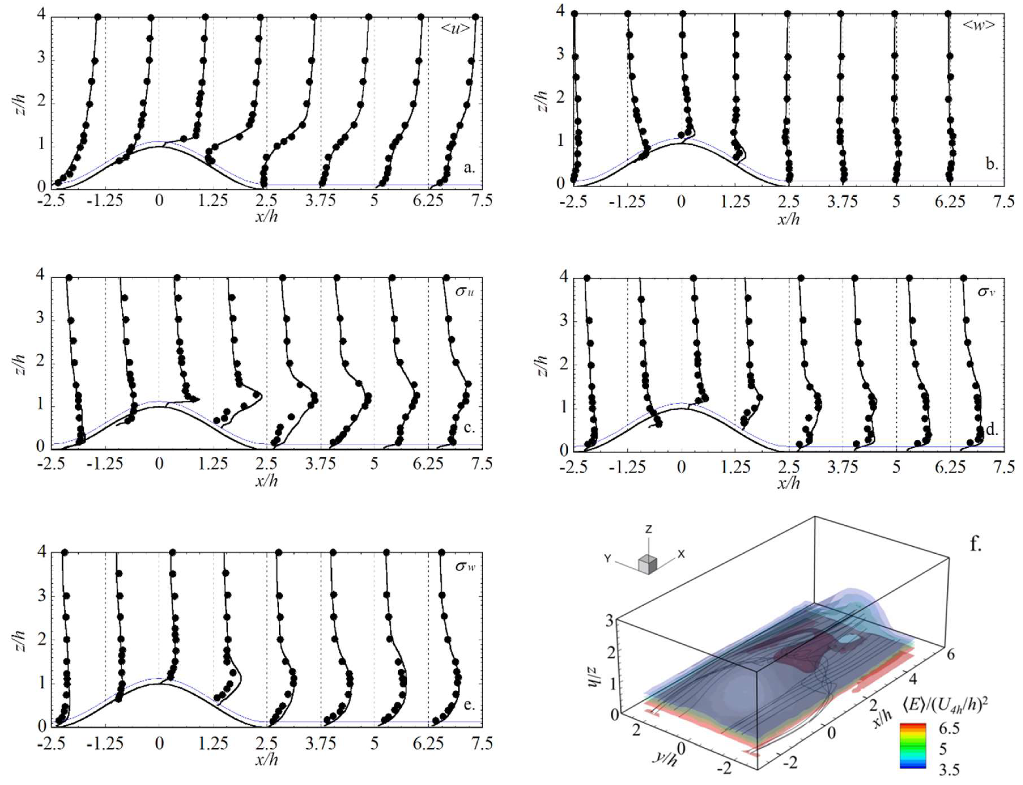
The profiles of u i and σ u i are plotted in Figure 7, where the normalization, using h and U4h, the same as the experiment, was adopted. The flow accelerates both in streamwise and vertical directions on the way up to the hill top. w reaches the maximum at x = −1h, which is due to the largest hill slope here. Still at x = −1h, the fluctuations of the flow in the canopy are the most energetic, which suggests that the upcoming flow becomes very unstable at the upwind hill side. This unstable feature is probably because it is much easier for the flow to penetrate the canopy due to the blockage effects of the hill. As a result, the interaction between the flow and the canopy becomes much stronger.
At the summit, x = 0, the speed-up of u is the largest. Interestingly, a sharp peak in the profile of σ u occurs at the canopy top of the summit. This should result from the ejection of the flow as well as the rapid distortion of the streamwise eddies. However, u i and σ u i quickly decrease to about 0 when the flow penetrates the canopy under the drag effects from the canopy, formulated by the drag force terms in the momentum–balance equations. When the flow propagates to the lee side of the hill, the mean velocities are distorted significantly. On one hand, inversion points on the profiles of u and w occur due to the presence of a recirculation bubble. On the other hand, the vertical gradient of u does not decrease monotonously as those upstream of the hill summit. In fact, u / z firstly decreases and then increases with the rise in the elevation, forming an inflection point, at which u / z reaches the maximum, suggesting large wind shear and turbulence productions. This can be confirmed by the near wake σ u profiles, of which the maximum is just located at the inflection points of the u profiles.
Additionally, similar to the flow over an isolated smooth 3D hill observed by Liu et al. [19], two peaks on σ v profiles appear, also for the rough 3D hill, with one located at the canopy top and the other in the shear layer region. Comparing the low-elevation peaks of σ v downstream and upstream of the hill, the magnitudes of the peaks are roughly identical, which differs with that in the smooth 3D hill case, implying different sources of low-elevation peaks of σ v . For the smooth case, Liu et al. concluded that the different rotation directions between the inner core and the outer core of the wake vortex are the sources [19]. For the rough one, however, due to the nearly same value between the near-ground peak σ v upstream and downstream the hill, the production of turbulence from the canopy should be the source. This also indicates the different coherent structures in the wakes of the smooth and rough hills.
Different from the 2D ridge, the flow fields over an isolated 3D hill are indeed three dimensional. The three-dimensional flow fields over a smooth 3D hill have been revealed and the coherent structures have been clarified in the study by Liu et al. [19]. However, the research considering flow fields over an isolated 3D hill with vegetation covered from a three-dimensional view is lacking. Before the presentation of the three-dimensional distributions of the parameters, it is worthwhile to have a general view about the structures of the mean flow fields over the 3D rough hill. As shown in Figure 7f, three enstrophy iso-surfaces with normalized values of 3.5, 4.5, 5.5, and 6.5 are shown. To illustrate the flow structures clearly, transparent effects are applied, and the streamlines determined by the space–time averaged velocities are plotted as well.
Surprisingly, the most energetic rotations were not located on the central plane y = 0, but 0.5h away from it. From the later discussion about the averaged vorticities, the rotations in vertical and streamwise directions were found to be the major sources of the large enstrophy. That is the reason why the strongest enstrophy does not occur at y = 0 plane, where only the mean spanwise vorticity has values because of the symmetry of the flow. In the far wake region, the shapes of the enstrophy iso-surfaces seem to be the projections of the 3D hill, and obviously the effects of the hill remain strong even at x = 5h. Furthermore, from the depicture of the streamlines, it can be found that the near-ground flow converges to the very center of the wake as it moves downstream from the lateral sides, and then its direction is changed upstream and upward in the recirculation bubble. Furthermore, we can see that the flow at relatively high elevations can hardly penetrate the bubble. However, the convergence of the flow to the y = 0 plane is still obvious due to the negative pressure in the central wake.
Furthermore, it is necessary to mention that the time-averaged flow fields should be symmetrical if the sampling time is sufficient. However, the symmetry of the flow can hardly be achieved in the numerical simulations, even when the sampling lasts for 400 time units. Therefore, space averaging is further carried out to obtain the symmetry of the flow. For the symmetrical parameters, such as u , w , σ u i , etc., ϕ = [ϕ (y) + ϕ (−y)]/2, and for the anti-symmetry parameters, such as v , ϕ = [ϕ (y) − ϕ (−y)]/2.
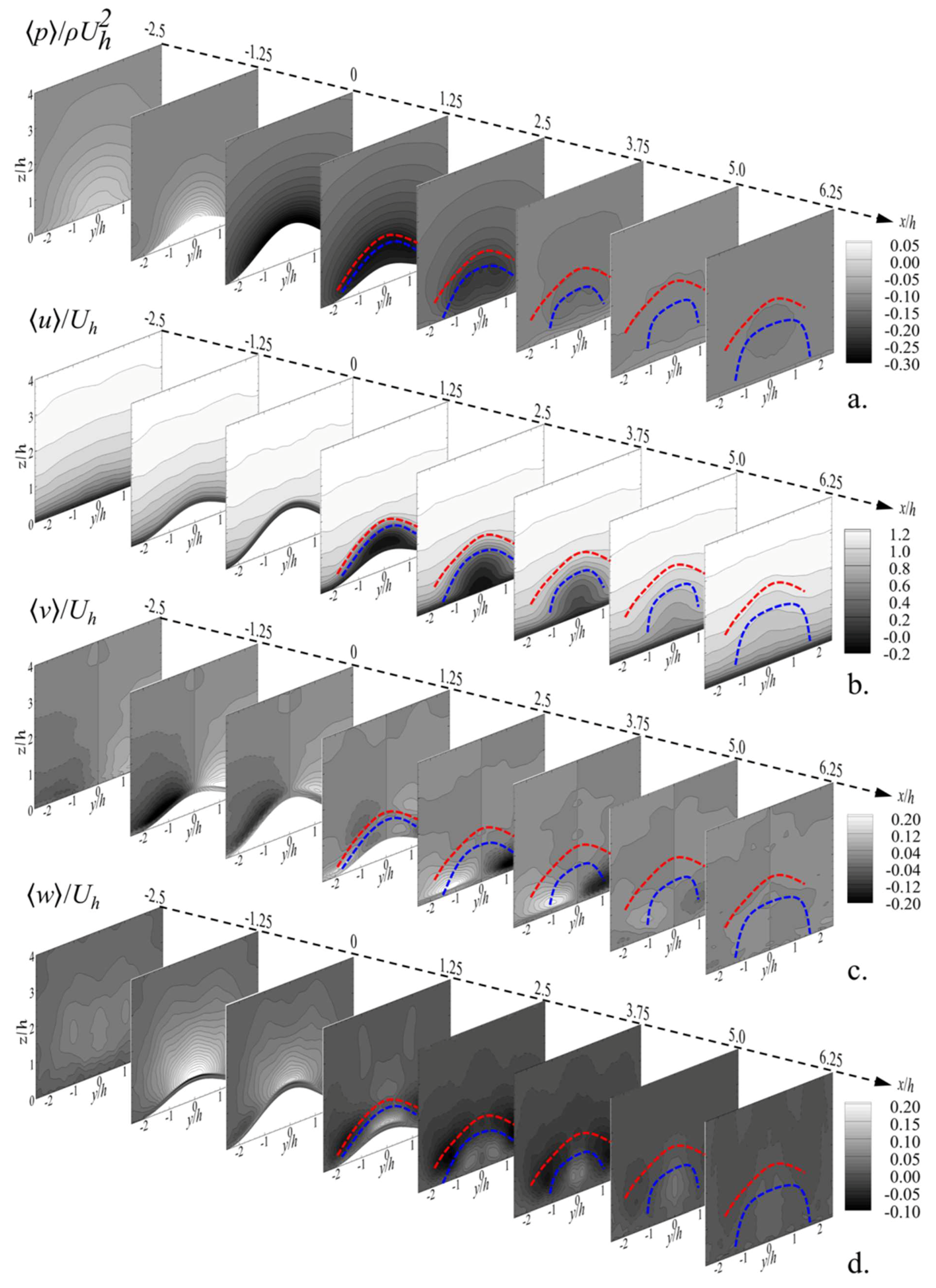
To illustrate the three-dimensional flow structures in a much clearer way, eight spanwise slices from x = −2.5 h to x = −6.25 h with a step size of 1.25 h were selected, which just coincide with the locations where the profiles in Figure 7 are shown. Each slice was centered at y = 0 h with a spanwise size of 5 h and vertical size of 4 h. The red dashed lines and the blue dashed lines superimposed on the slices indicate the locations where the flow recovers to the inactive boundary layer (IBL) flow and the locations where TKE shows the peak, respectively. Accordingly, the region enclosed by the red and blue dashed lines can be considered as the shear-layer region. In the present study, the wake depth (hw) was quantitatively calculated as | u down(hw) −   u up(hw)| / u up(hw) < 0.05, where u down is u downstream of the hill, and u up is u upstream of the hill.
From the averaged parameters shown in Figure 8, some important features were not captured by the vertical profiles on y = 0 slice. Firstly, it is apparent that the area influenced by the topography not only increases in the vertical direction, but also expands in the spanwise direction with the increase in x, while this influence is weakened and almost dismisses when x ≈ 12h (not shown in the figures). Secondly, it is important that v is accelerated both at the upwind and lee sides of the hill. The magnitude of v can even reach 0.2 Uh. It can be further found that the streamwise distance to the hill center of the upstream peak v , 1.25 h, differs from that downstream, 2.5h, which results from the appearance of the recirculation bubble. This recirculation bubble acts as an obstacle, and the flow majorly moves in the region outside of the bubble. The positive v in −y part and the negative v in +y part imply the presence of a pair of vortices pointing to positive and negative vertical directions, respectively. Finally, on the way up to the summit, w shows sole peak at y = 0, while two pairs of peaks w emerged downstream from the hill crest. One pair was located at the shear layer with negative value, and the other located in central wake with positive value, revealing the presence of the vortices pointing to the streamwise direction.
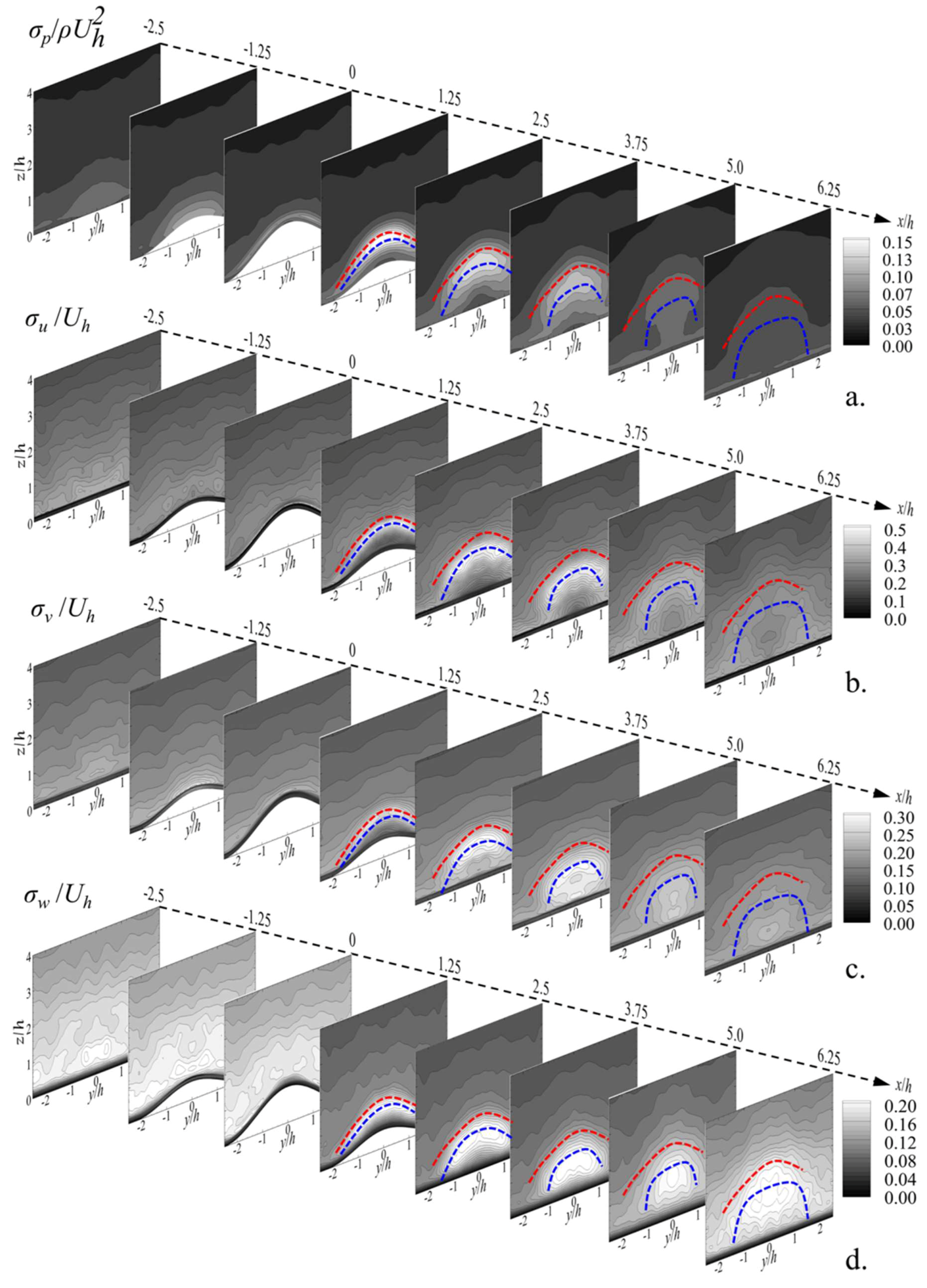
Similar distributions can be detected for σ p , σ u , and σ v , as shown in Figure 9. The concentrations of σ p , σ u , and σ v in the shear layer are obvious. However, the distributions for σ w are distinct, whose peaks are centered just below the shear layer center. In addition, it is worth mentioning that σ p and σ u i suddenly increase at the upwind footage of the hill, revealing the presence of a horseshoe vortex. This horseshoe vortex was also identified in the smooth 3D hill case in the study by Liu et al. [19], implying that the disturbance of the flow from the canopy cannot eliminate the formation of the horseshoe vortex due to the topography.

3.4. TKE Budget

Studying roughness–turbulence interactions is one of the motivations of the present study and the TKE budget provides information about the gain or loss of the TKE, as has been examined in the studies considering the effects of roughness or the particle bed on the turbulent flow fields [20,21,22]. In those studies, it was found that the roughness modulates the near-bed turbulence; produces streamwise structures, which undergo distortion and breaking; and reduce the large-scale anisotropy. A double averaging of the flow field reveals spatial inhomogeneities at the roughness scale and alternate paths of energy transportation in the turbulent kinetic energy (TKE) budget. The TKE budget is formulated as:
u ¯ j k x j = 1 ρ u i   p ¯ x i 1 2 u j u j u i x i   u i u j u ¯ i x j     ν u i x j u i x j
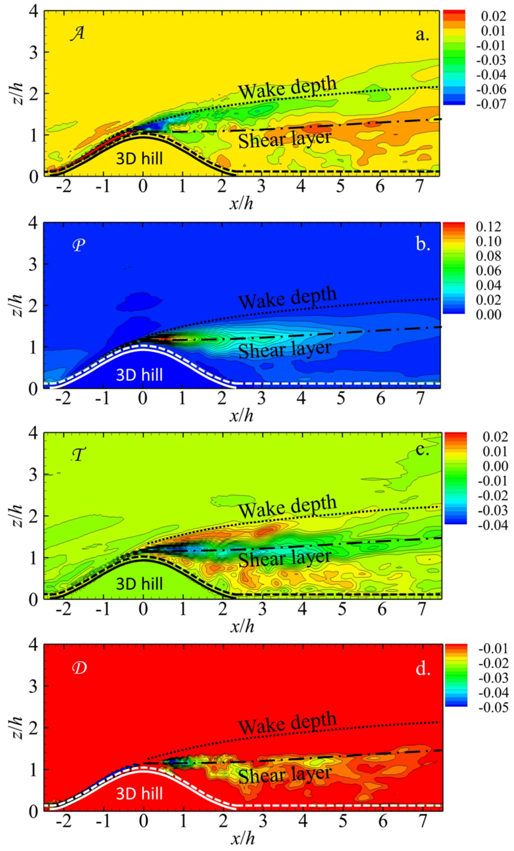
where the advection term A is u i k x j , the pressure diffusion term, 1 ρ u i p x i , is too small to be considered, the turbulence transportation term T is 1 2 u j u j u i x i , the turbulence production term P is   u i u j u ¯ i x j , and the dissipation term D is   ν u i x j u i x j .
Their distributions on the slice of y = 0 are shown in Figure 10. The dominant term was found to be the turbulence production. A formula based on a turbulence generation term, this value is primarily determined by the shear of the average flow. Moreover, kinetic energy is generated in the opposite direction of the Reynolds stress, which not only eliminates the kinetic energy of the average flow, but also transfers the kinetic energy that is eliminated to the fluctuating velocity fields. Therefore, it is apparent that the maximum of the shear production P is at the entry of the flow into the hill wake, where a sudden flow ejection occurs and the shear layer begins to develop. Apart from the concentrations of the turbulence production in the shear layer region, a secondary concentration of P can be identified at the canopy top. The production P and dissipation D are directly responsible for the gain and loss of k in the transport equation, respectively. It can be seen that the dissipation is negative in the global process. This is because the turbulent dissipation acts as a sink for the TKE budget. It can act as a resistance to fluctuating stress and can also convert kinetic energy into internal energy. Interestingly, different from P, the concentration of D is observed at the locations just below the shear layer. Moreover, there are abruptly no dissipations above the shear layer, revealing the much more organized instantaneous turbulence structures here. The secondary dominant term is A. It is negative in the shear layer but positive in the wake core region, whose distribution is similar to the turbulence transportation term.

3.5. Spectrum

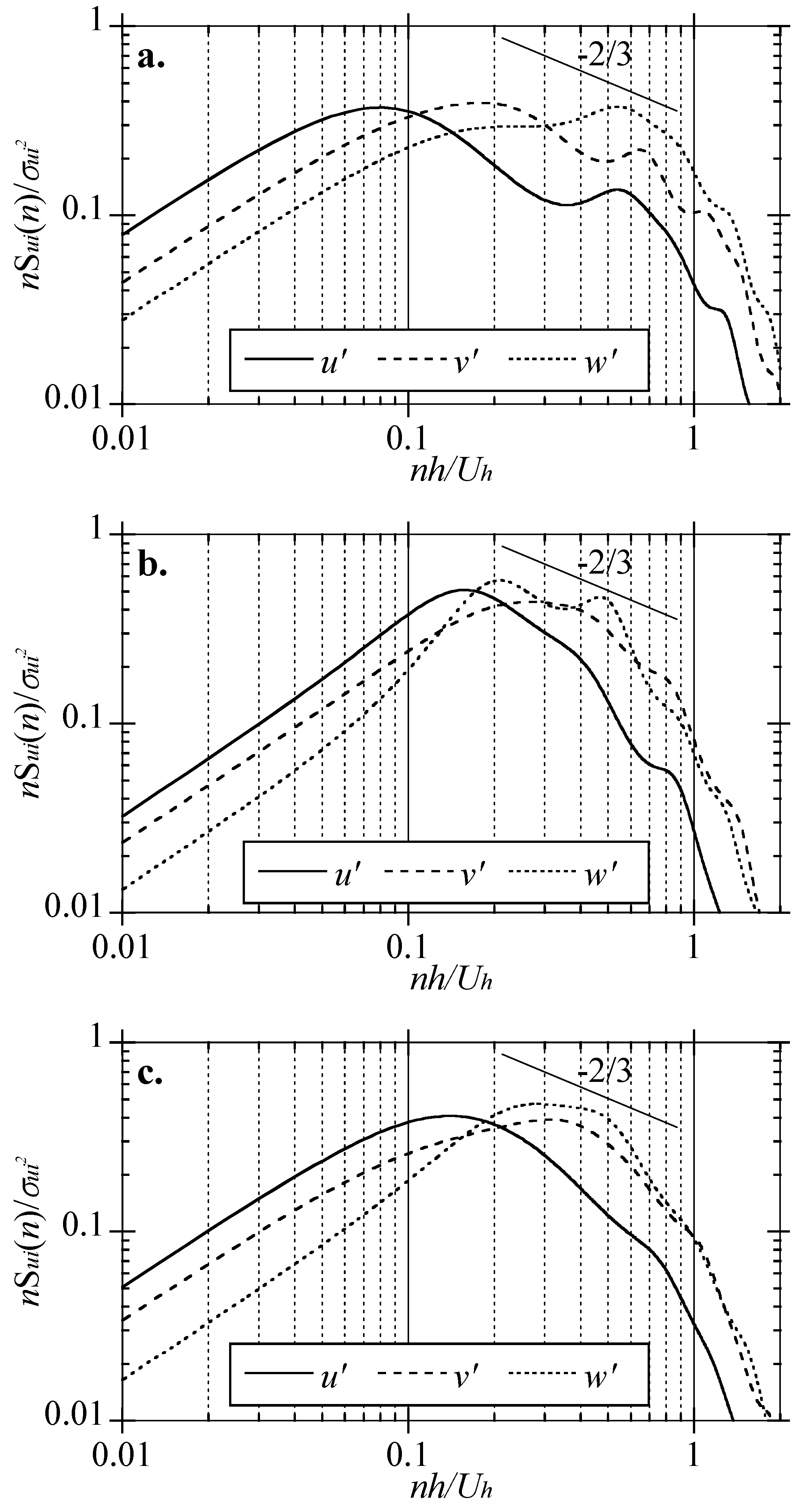
Spectral analysis provides information about how energetic the structures are, as a result perhaps shedding some light on the dynamics of the eddy motions. Figure 11 displays the one-dimensional pre-multiplied spectra of three velocity components n S u , n S v , and n S w , further normalized by u 2 , v 2 , and w 2 , respectively. The horizontal axis is normalized by Uh/h, making it convenient to clarify the relative sizes of the eddies to those of the hills. The time signals of the flow at P1~P3 were recorded over a period of 400 time units. The maximum entropy method (MEM) was employed to obtain smoothed Su. MEM is an extrapolated spectral density estimation technique based on segments of known autocorrelation functions with unknown lags [23,24,25]. In particular, it is necessary to mention that with a restricted number of poles, MEM will smooth the spectrum somewhat, which is important to identify the peaky regions in the plotting. However, if the number of poles is extremely small, the important information of the energetic motions may be smoothed, while if the number of poles is extremely large, round-off error can be a problem, leading to the introduction of additional peaks shifting with a phase of sine wave. Finally, 250 poles were selected to achieve a compromise between the smoothness of the spectra and the width of the frequency covered, which has also been selected in the previous study by Liu et al. [14].
In general, S u i in the present LES exhibits a −2/3 slope in the inertial subrange, covering at least one decade, which is in consistent with Kolmogorov’s hypothesis. However, there is a steep decrease beyond this inertial range (nh/Uh > 1), suggesting that the present LES do not have the capabilities to resolve the small-scale eddies in a broad dissipation range due to the filtering effects from the SGS model. The spectra of streamwise, spanwise, and vertical velocities at P1 peak at different wavenumbers, which are about 0.1, 0.2, and 0.6, respectively. Whereas, moving the reference point to P2, a clear shift of peak Su to high wavenumber region is identified, indicating the large-scale streamwise velocity breaks into smaller scales at the hill top. This shift can also be observed in the spectrum of the spanwise velocity. It is of interest that at the crest, the energies of the fluctuating velocities are condensed, which is revealed by steeper caves on the spectrum distributions, suggesting the generation of the energetic coherent structures. Significantly, the peak spectra of the three velocity components seem to occur at nearly the same wavenumber (nh/Uh 0.2). Further moving the reference point to P3, the spectra curves do not vary much in comparison with those at P2. However, the curves are significantly smoothened at P3 and the peaks of the spectra are much easier to be identified. It is the signature that the coherent structures in the IBL flow are seldom transported into the shear layer. The similar spectra at P2 and P3 also suggest that the topography-generated coherent structures have significant effects on the velocities upstream.

4. Conclusions

In the present study, the 3D mean and turbulent flows over a hill with vegetation cover were simulated and analyzed. The major conclusions are summarized as follows.
  • The production of turbulence from the canopy is the source of the secondary peak spanwise fluctuations in the hill wake. Moreover, two pairs of peak vertical velocity downstream of the hill crest were identified from the three-dimensional view of the mean velocities. One pair was located at the shear layer, and the other located in the central wake.
  • The energies of the fluctuating velocities are condensed, represented by steeper caves on the spectrum distributions, suggesting the generation of the energetic coherent structures. Additionally, the similar spectra at P2 and P3 are the indications that the topography-generated coherent structures have significant effects on the velocities upstream.
  • A pair of the lateral shedding are the reason for the double peaks on the distributions of σu, Sku, Kuu, and Ruu. The turbulence structures in the hill consist of the lateral shedding, the shedding from the hill crest, as well as the canopy-induced rotations. The lateral shedding and the shedding from the hill crest yield an area with quite small velocities and weak vortices, leading to the formation of a dead flow area.

Author Contributions

Conceptualization, Z.L. and Y.H.; methodology, Z.L.; software, Y.H.; validation, W.W., Z.L. and Y.F.; formal analysis, Y.F.; investigation, Q.Z.; resources, Z.L.; data curation, Q.Z.; writing—original draft preparation, Z.L.; writing—review and editing, Y.H.; visualization, Y.F.; supervision, Z.L.; project administration, Z.L.; funding acquisition, Z.L.

Funding

This research was funded by National Key Research and Development Plan of China, grant number 2016YFE0127900, National Natural Science Foundations of China, grant number 51608220, and the Project of Innovation-driven Plan in Huazhong University of Science and Technology, grant number 2017KFYXJJ141.

Conflicts of Interest

The authors declare no conflict of interest.

References

  1. Politis, E.S.; Prospathopoulos, J.; Cabezon, D.; Hansen, K.S.; Chaviaropoulos, P.K.; Barthelmie, R.J. Modeling wake effects in large wind farms in complex terrain: The problem, the methods and the issues. Wind Energy 2011, 15, 161–182. [Google Scholar] [CrossRef]
  2. Carvalho, A.C.; Carvalho, A.; Gelpi, I.; Barreiro, M.; Borrego, C.; Miranda, A.I.; Pérez-Muñuzuri, V. Influence of topography and land use on pollutants dispersion in the Atlantic coast of Iberian Peninsula. Atmos. Environ. 2006, 40, 3969–3982. [Google Scholar] [CrossRef]
  3. Davenport, A.G.; King, J.P.C. The influence of topography on the dynamic wind loading of long span bridges. J. Wind Eng. Ind. Aerod. 1990, 36, 1373–1382. [Google Scholar] [CrossRef]
  4. Matusick, G.; Ruthrof, K.X.; Brouwers, N.C.; Hardy, G.S.J. Topography influences the distribution of autumn frost damage on trees in a Mediterranean-type Eucalyptus forest. Trees 2014, 28, 1449–1462. [Google Scholar] [CrossRef] [Green Version]
  5. Lopes, A.M.G.; Cruz, M.G.; Viegas, D.X. FireStation—An integrated software system for the numerical simulation of fire spread on complex topography. Environ. Modell. Softw. 2002, 17, 269–285. [Google Scholar] [CrossRef]
  6. Dupont, S.; Brunet, Y. Edge Flow and Canopy Structure: A Large-Eddy Simulation Study. Bound. Layer Meteorol. 2008, 126, 51–71. [Google Scholar] [CrossRef]
  7. Takahashi, T.; Ohtsu, T.; Yassin, M.F.; Kato, S.; Murakami, S. Turbulence characteristics of wind over a hill with a rough surface. J. Wind Eng. Ind. Aerod. 2002, 90, 1697–1706. [Google Scholar] [CrossRef]
  8. Cao, S.; Tamura, T. Experimental study on roughness effects on turbulent boundary layer flow over a two-dimensional steep hill. J. Wind Eng. Ind. Aerod. 2006, 94, 1–19. [Google Scholar] [CrossRef]
  9. Cao, S.; Tamura, T. Effects of roughness blocks on atmospheric boundary layer flow over a two-dimensional low hill with/without sudden roughness change. J. Wind Eng. Ind. Aerod. 2007, 95, 679–695. [Google Scholar] [CrossRef]
  10. Dupont, S.; Brunet, Y.; Finnigan, J.J. Large-eddy simulation of turbulent flow over a forested hill: Validation and coherent structure identification. Q. J. R. Meteorol. Soc. 2008, 134, 1911–1929. [Google Scholar] [CrossRef]
  11. Ishihara, T.; Fujino, Y.; Hibi, K. A wind tunnel study of separated flow over a two-dimensional ridge and a circular hill. J. Wind Eng. 2001, 89, 573–576. [Google Scholar]
  12. Ishihara, T.; Hibi, K. Numerical study of turbulent wake flow behind a three-dimensional steep hill. Wind Struct. 2002, 5, 317–328. [Google Scholar] [CrossRef]
  13. Tamura, T.; Cao, S.; Okuno, A. LES Study of Turbulent Boundary Layer Over a Smooth and a Rough 2D Hill Model. Flow Turbul. Combust. 2007, 79, 405–432. [Google Scholar] [CrossRef]
  14. Liu, Z.; Ishihara, T.; Tanaka, T.; He, X.H. LES study of turbulent flow fields over a smooth 3-D hill and a smooth 2-D ridge. J. Wind Eng. Ind. Aerod. 2016, 153, 1–12. [Google Scholar] [CrossRef]
  15. Ferziger, J.H.; Peric, M. Computational Method for Fluid Dynamics; Springer: Berlin, Germany, 2002. [Google Scholar]
  16. Iizuka, S.; Kondo, H. Large-eddy simulations of turbulent flow over complex terrain using modified static eddy viscosity models. Atmos. Environ. 2006, 40, 925–935. [Google Scholar] [CrossRef]
  17. Lee, S.H.; Sung, H.J. Direct numerical simulation of the turbulent boundary layer over a rod-roughened wall. J. Fluid Mech. 2007, 584, 125–146. [Google Scholar] [CrossRef] [Green Version]
  18. Ishihara, T.; Qi, Y.H. Numerical study of turbulent flow fields over steep terrains by using a modified delayed detached eddy simulation. Bound. Layer Meteorol. 2018, 170, 1–24. [Google Scholar] [CrossRef]
  19. Liu, Z.; Cao, S.; Liu, H.; Ishihara, T. Large-eddy simulations of mean and turbulent flow and coherent structures over an isolated 3D hill. Bound. Layer Meteorol. 2018, 170, 1–27. [Google Scholar]
  20. Ghodke, D.C.; Apte, V.S. DNS study of particle-bed–turbulence interactions in an oscillatory wall-bounded flow. J. Fluid Mech. 2018, 792, 232–251. [Google Scholar] [CrossRef]
  21. Ghodke, D.C.; Apte, V.S. Roughness effects on the second-order turbulence statistics in oscillatory flows. Comput. Fluids. 2018, 162, 160–170. [Google Scholar] [CrossRef]
  22. Ghodke, D.C.; Apte, V.S. Spatio–temporal analysis of hydrodynamic forces on the particle bed in an oscillatory flow environment. J. Fluid Mech. 2018, 841, 167–202. [Google Scholar] [CrossRef]
  23. Childers, D. Modern Spectrum Analysis; Chapter II; IEEE Press: New York, NY, USA, 1978. [Google Scholar]
  24. Kay, S.; Marple, S. Spectrum Analysis: A Modern Perspective. Proc. IEEE 1981, 69, 1380–1419. [Google Scholar] [CrossRef]
  25. Press, W.; Teukolsky, S.; Vetterling, W.; Flanney, B. Numerical Recipes 3rd Edition: The Art of Scientific Computing; Cambridge University Press: Cambridge, UK, 2007; pp. 681–685. [Google Scholar]
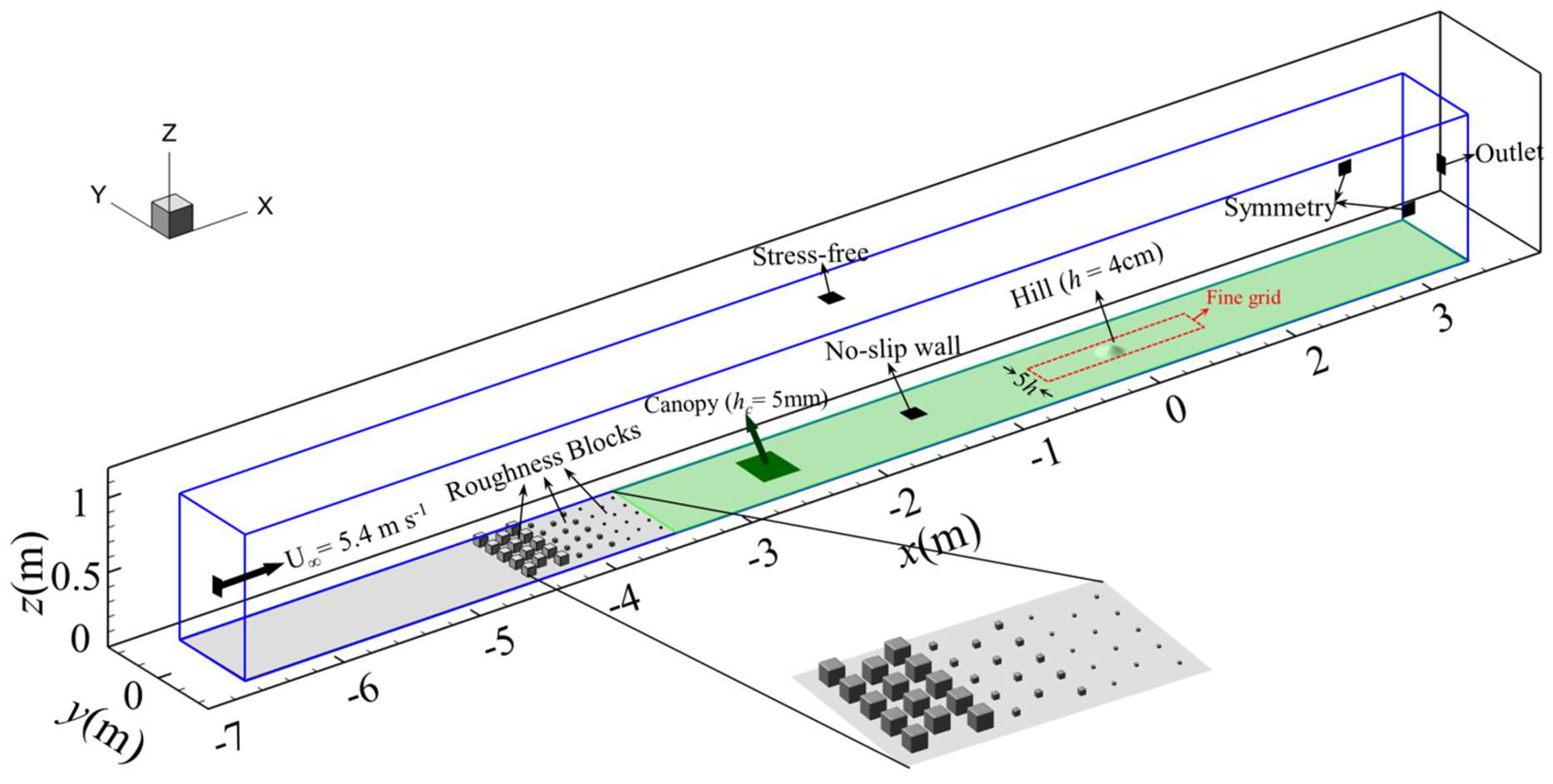
Figure 1. Configurations of the numerical model. The volume enclosed by solid blue lines is the computational domain and the area enclosed by the red dashed rectangular is the fine grid region, 5 h in width and 30 h in length. The original point (0, 0, 0) of the model is at the center of the fine grid, where the hill with a height of 40 mm is mounted. The solid dark squares with arrows indicate the boundary conditions. The green area indicates the regions with a vegetation canopy cover.
Energies 12 03624 g001
Figure 2. Mesh on the vertical slice crossing the center of the topographies.
Energies 12 03624 g002
Figure 3. Distributions of mean skin friction coefficient around the hill.
Energies 12 03624 g003
Figure 4. The instantaneous flow fields with the absence of the hill. The visualization by the normalized vorticity in spanwise direction, ωyh/Uh, is applied. Two iso-surfaces with ωyh/Uh = −0.01 and ωyh/Uh = 0.01 are plotted. The grid sizes and the grid spacing ratio are sketched.
Energies 12 03624 g004
Figure 5. Vertical profiles of (a) normalized mean streamwise velocity, u / U 4 h , in which y axis is plotted in logarithmic form and (b) normalized fluctuations of streamwise component, σu/U4h, spanwise component, σv/U4h, and vertical component, σw/U4h at x = 0 and y = 0 in the absence of the hills. The data from the wind tunnel experiment by Ishihara et al. [11] are superimposed to verify the accuracy of the generated upwind turbulent boundary layer (TBL) flow. The dotted line exhibits the canopy top.
Energies 12 03624 g005
Figure 6. Instantaneous flow fields at (a) tUh/h = 116 and (b) tUh/h = 118 visualized by iso-surfaces of Q-criteria with normalized values 3.0 and −3.0. A 50% transparent effect was applied for the iso-surfaces of Q values to show the flow structures clearly. The iso-surfaces are further colored by the instantaneous streamwise velocity. The red dashed lines represent the center of the vortices shedding from the lateral sides of the hill and the yellow dashed lines show the vortices shedding from the hill crest. The centers of the vortices were determined by velocity gradient eigenmodes method. x and y axes are normalized by h. (c) Sketch of the flow structure. V1 and V4 are vortices induced by the canopy, V2 is the vortex distorted by the topography, V3 is the vortex shedding from the hill crest, V5 is the vortex shedding from the lateral sides of the hill.
Energies 12 03624 g006
Figure 7. Vertical profiles of: (a) normalized mean streamwise velocity, u / U 4 h ; (b) normalized mean vertical velocity, w / U 4 h ; (c) normalized r.m.s of fluctuating streamwise velocity, σ u / U 4 h ; (d) normalized r.m.s of fluctuating streamwise velocity, σ v / U 4 h ; (e) normalized r.m.s of fluctuating vertical velocity, σ w / U 4 h , at x equals to −2.5h–6.25h with a step size of 1.25 h. The unit in the x-axis represents the unit in the plotting of u / U 4 h and w / U 4 h , and 0.2 in the plotting of σ u / U 4 h , σ v / U 4 h and σ w / U 4 h . The solid lines are from the present LES and the circles are from the wind tunnel experiment by Ishihara et al. [12]. The averaged three-dimensional flow structures are shown in Figure 7f by the normalized mean enstrophy with the mean streamlines superimposed. The blue solid line indicates the canopy top. x, y, and z axes have been normalized by h.
Energies 12 03624 g007
Figure 8. Distributions of normalized (a) averaged pressure, p   /   ρ U h 2 ; (b) averaged streamwise velocity, u / U h ; (c) averaged spanwise velocity, v / U h ; (d) averaged vertical velocity, w / U h , on the slices of x = −2.5h–6.25h with a step size of 1.25h. The width of the slices is 5h centering at the y = 0, and the height is 4h. The red dashed lines represent the upper boundary of the wake and the blue dashed lines indicate the center of the shear layer. x, y, and z axes have been normalized by h.
Energies 12 03624 g008
Figure 9. Distributions of normalized (a) r.m.s of fluctuating pressure, σ p /   ρ U h 2 ; (b) streamwise velocity, σ u / U h ; (c) spanwise velocity, σ v / U h ; (d) vertical velocity, σ w / U h , on the slices of x = −2.5h–6.25h with a step size of 1.25h. The width of the slices is 5h, centering at the y = 0, and the height is 4h. The red dashed lines indicate the upper boundary of the wake and the blue dashed lines indicate the center of the shear layer. x, y, and z axes have been normalized by h.
Energies 12 03624 g009
Figure 10. Distributions of normalized turbulence kinetic energy (TKE) budget on the slice of y = 0 with x-axis ranging from −2.5h to 7.5h and z-axis ranging from 0h to 4h, (a) advection, A; (b) turbulence production, P; (c) turbulence transportation, T, and (d) dissipation, D. The solid line indicates the hill shape, dashed line is the canopy top, dotted line shows the upper boundary of the wake, and the dash-dotted line implies the center of the shear layer.
Energies 12 03624 g010
Figure 11. One-dimensional pre-multiplied spectra of three velocity components n S u , n S v , and n S w at the monitoring points: (a) P1; (b) P2; and (c) P3. The pre-multiplied spectra n S u , n S v , and n S w are further normalized by u 2 , v 2 , and w 2 , respectively, and the frequency n is normalized by Uh/h. The inclined lines with a slope of 2/3 are drawn to show the inertial subrange of the spectra.
Energies 12 03624 g011