Article

Economic Impact of Energy Consumption Change Caused by Global Warming

1
Centre for Applied Macroeconomic Analysis, Crawford School of Public Policy, Australian National University, Canberra, ACT 2601, Australia
2
P.Eng. (Non-Practicing), Life Member of The Association of Professional Engineers and Geoscientists of Alberta (APEGA), 1500 Scotia One, 10060 Jasper Avenue NW, Edmonton, AB T5J 4A2, Canada
*
Author to whom correspondence should be addressed.
Energies 2019, 12(18), 3575; https://doi.org/10.3390/en12183575
Submission received: 28 June 2019 / Revised: 23 August 2019 / Accepted: 27 August 2019 / Published: 19 September 2019
(This article belongs to the Section C: Energy Economics and Policy)

Abstract

:
This paper tests the validity of the FUND model’s energy impact functions, and the hypothesis that global warming of 2 °C or more above pre-industrial times would negatively impact the global economy. Empirical data of energy expenditure and average temperatures of the US states and census divisions are compared with projections using the energy impact functions with non-temperature drivers held constant at their 2010 values. The empirical data indicates that energy expenditure decreases as temperatures increase, suggesting that global warming, by itself, may reduce US energy expenditure and thereby have a positive impact on US economic growth. These findings are then compared with FUND energy impact projections for the world at 3 °C of global warming from 2000. The comparisons suggest that warming, by itself, may reduce global energy consumption. If these findings are correct, and if FUND projections for the non-energy impact sectors are valid, 3 °C of global warming from 2000 would increase global economic growth. In this case, the hypothesis is false and policies to reduce global warming are detrimental to the global economy. We recommend the FUND energy impact functions be modified and recalibrated against best available empirical data. Our analysis and conclusions warrant further investigation.

Graphical Abstract

1. Introduction

There is a scientific hypothesis and political acceptance [1] that global warming of 2 °C or more above pre-industrial times would have a negative impact on global economic growth. This hypothesis is supported by economic models that rely on impact functions and many assumptions. However, the data needed to calibrate the impact functions is sparse, and the uncertainties in the modelling results are large [2,3]. The negative overall impact projected by at least one of the main models, Climate Framework for Uncertainty, Negotiation and Distribution (FUND) [4], is mostly due to one impact sector – energy consumption. However, the projected negative impact seems to be at odds with empirical data. If this paper’s findings from the empirical energy consumption data are correct, and if the impact functions for the non-energy sectors are correct, then the overall economic impact of global warming would be beneficial. If true, the implications for climate policy are substantial.
Integrated Assessment Models (IAM) approximately reproduce the projections from the Global Climate Models (GCM) and apply impact functions to estimate the economic impacts of global warming. The impact functions are derived from and calibrated to what the developers assess are the most suitable studies of the impacts. The impact functions require many assumptions, including projections of population, gross domestic product (GDP), per capita income, elasticities and technology progress in energy provision.
Various studies conclude that the impact functions (also called damage functions) used in the IAMs are derived from inadequate empirical data. For instance, Pindyck [5] (p. 11) says “when it comes to the damage function, however, we know almost nothing, so developers of IAMs can do little more than make up functional forms and corresponding parameter values. And that is pretty much what they have done.” According to Kolstad et al. [2] (p. 258), the IAM damage functions “are generated from a remarkable paucity of data and are thus of low reliability”. The National Academies of Sciences, Engineering and Medicine (NAS) [3] (p. 261) says FUND [4] needs further justification for the damage functions, the adaptation assumptions for the different sectors, the regional distribution of damages, and the parametric uncertainties overall. Tol [6] says the impact of climate change has not received sufficient attention; he says “there is either very little solid evidence, no conclusive evidence, or no quantification of welfare impacts”.
NAS [3] reviews the damage functions of the three main IAMs, discusses alternative approaches, reviews recent literature on damage estimation, and offers recommendations for a new damage module. It says that much of the literature on which the damage functions are based is dated and, in many cases, does not reflect recent advances in the scientific literature. For example, the FUND energy impact parameters are calibrated to reproduce the results of the 1996 papers by Downing et al. [7,8] and the income elasticity results of the 1995 paper by Hodgson and Miller [9].
FUND [4] is one of the three most cited IAMs; Bonen et al. [10], National Research Council [11] and NAS [3] compare them. FUND is the most complex. FUND disaggregates by sixteen world regions and eight main impact sectors (agriculture, forestry, water resources, sea level rise, ecosystems, health, extreme weather, and energy consumption). This enables analysts to conduct sensitivity analyses and to separately test individual impact functions.
Tol [12] used the national version of FUND3.6 to backcast the economic impact of global warming for these sectors for the 20th century and projected the impacts for the 21st century. Tol fitted the backcast results to observations of 20th century sectoral impacts (Tol [13]). Tol [12] is an important study because it estimates the impacts for the most significant impact sectors, globally and by region. It also estimates the total impact on all sectors. 
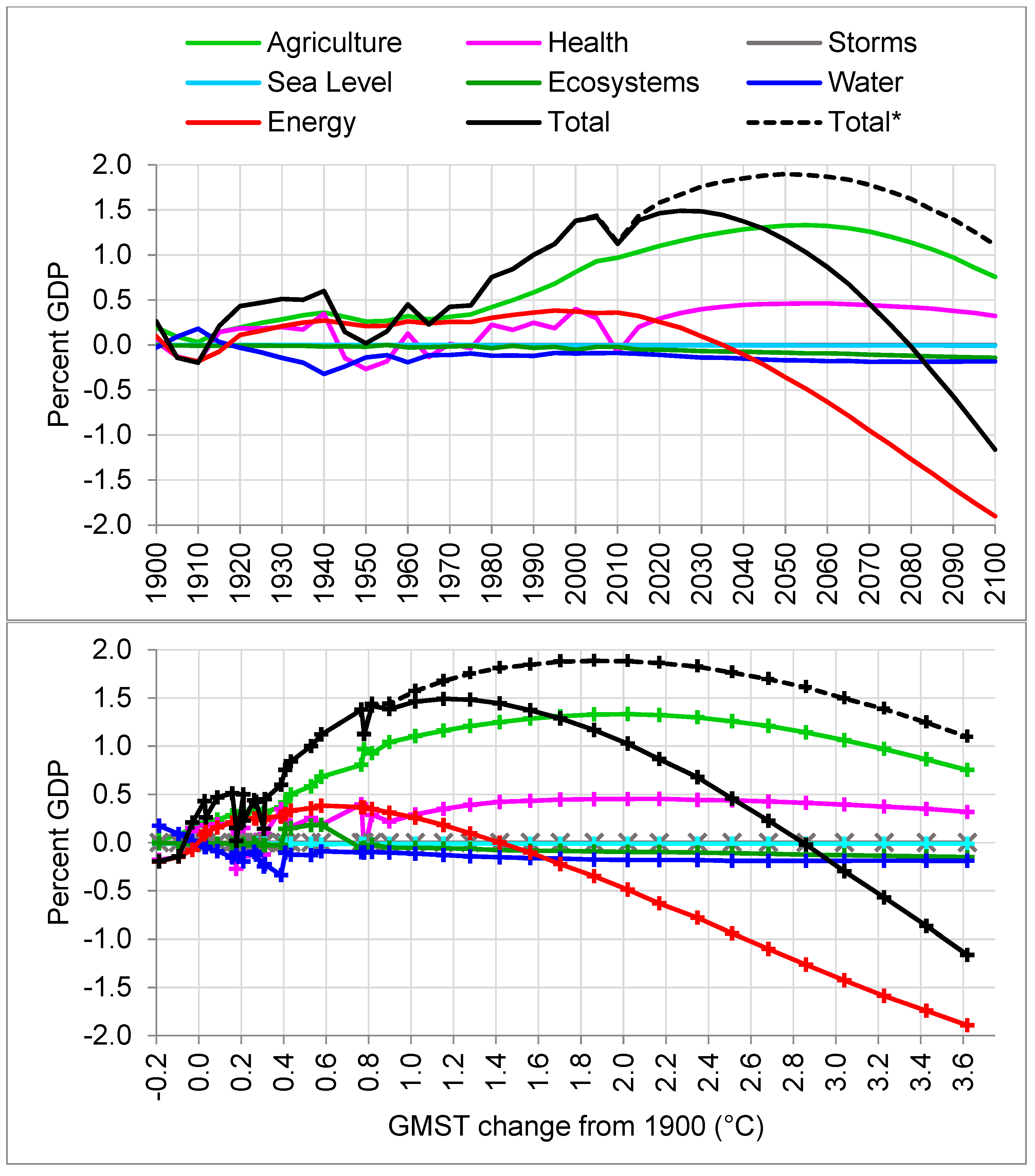
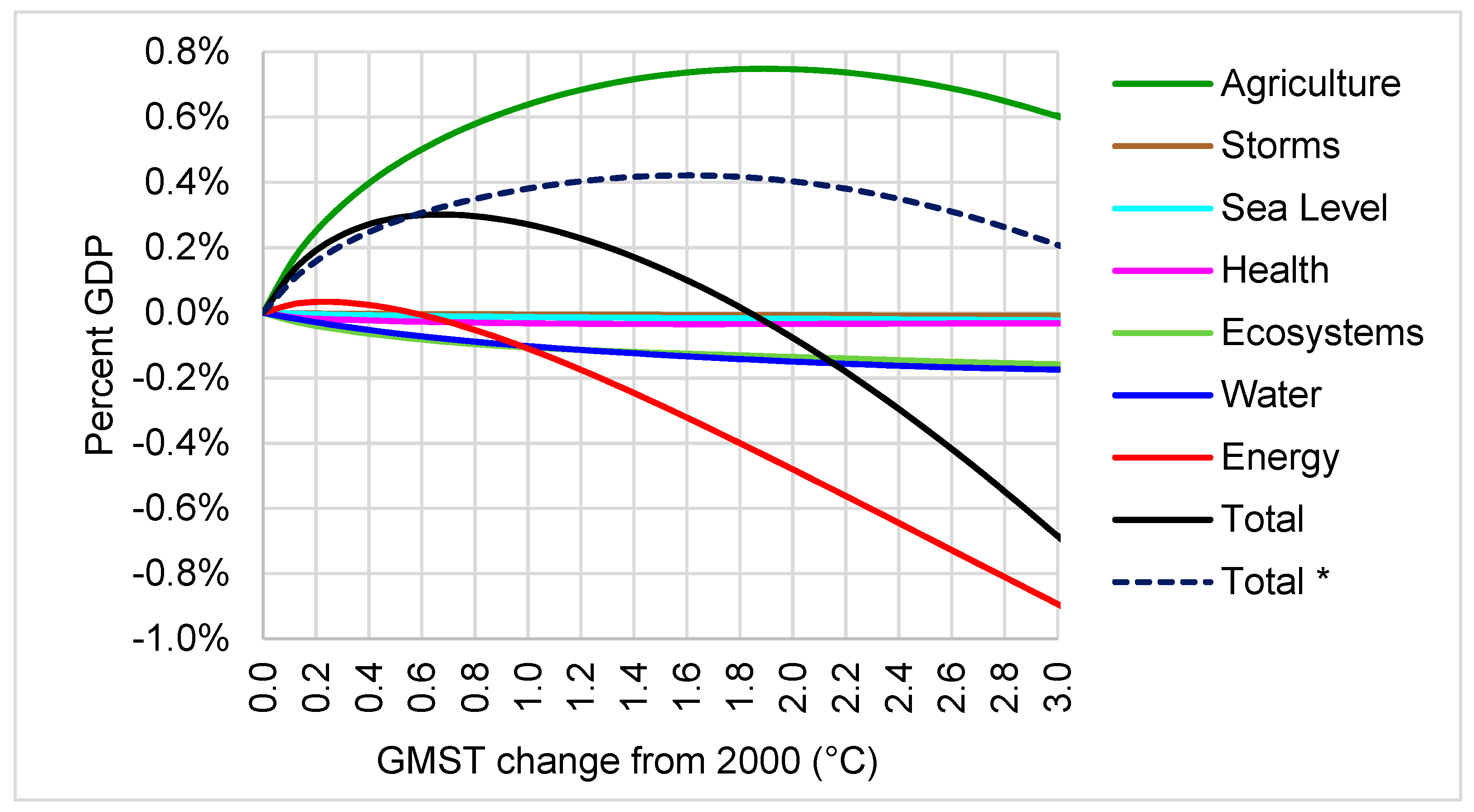
Figure 1 (adapted from Figure 3 in Tol [12]) shows the backcast (observed) and projected economic impact of global warming by sector. (We have added the ‘Total’ and ‘Total*’ lines. ‘Total’ is digitized from Tol [12] Figure 2. ‘Total*’ is the sum of all the backcast (observed) historical impacts from 1900 to 2000, and all projected sectoral impacts except energy from 2000 to 2100).
The bottom panel of Figure 1 suggests that an increase of up to around 4 °C Global Mean Surface Temperature (GMST) above pre-industrial times would be beneficial for the total of all sectors if the projected energy impacts for 2000–2100 are excluded. Energy consumption is projected to have a substantial negative impact during the 21st century; in fact, its negative impact exceeds the total impact of all other sectors, which is positive, from about 2080.
The striking change in trend of the energy impact at the turn of the century inspired this study. The trend was positive as GMST increased by 0.61 °C during the 20th century [13] but FUND projects it will be substantially negative for the 21st century as GMST is projected to increase further. That is, whereas the observations for 1900–2000 show the impacts were positive, FUND projects continued global warming would have negative impacts for the global economy.
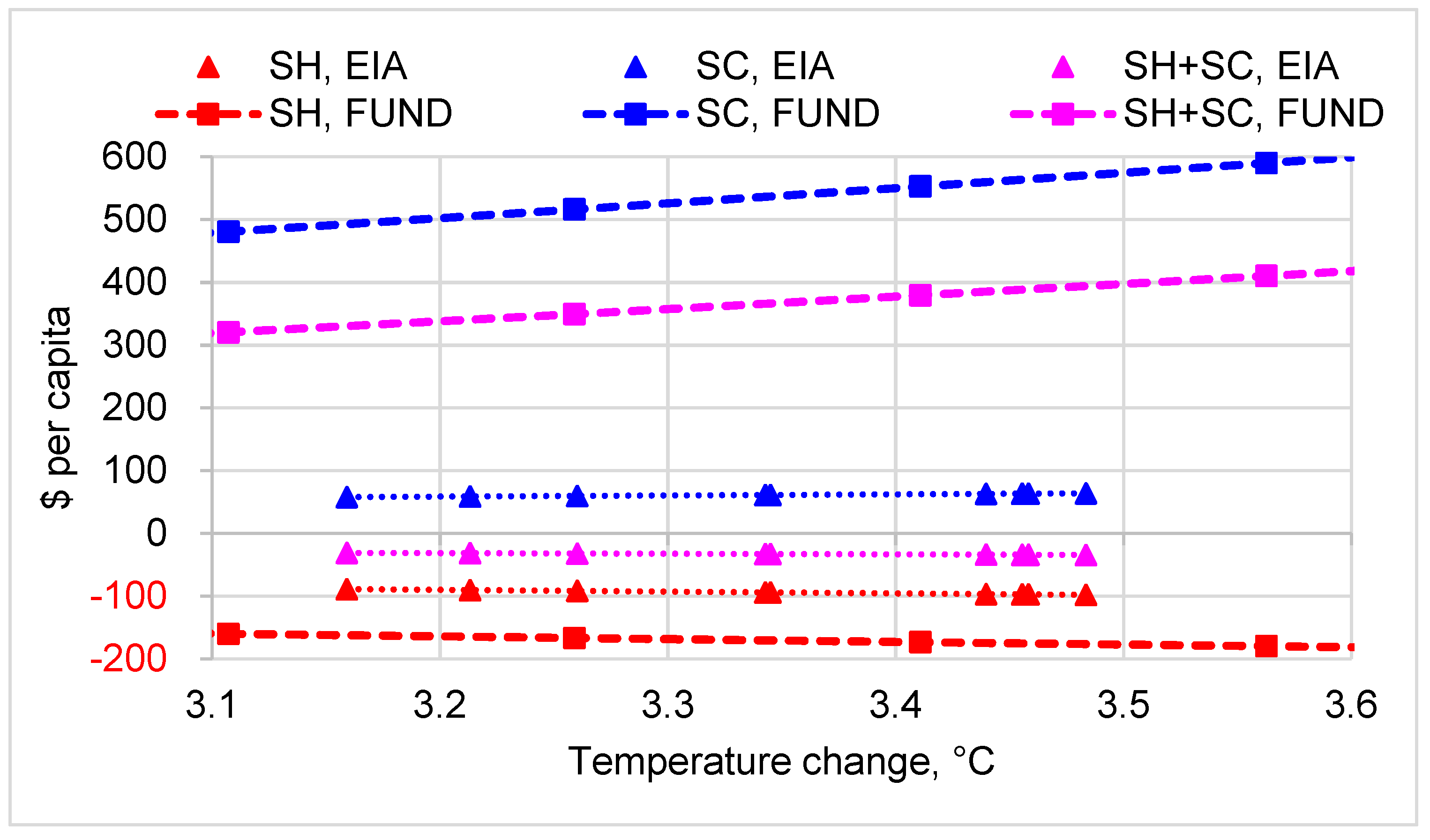
Contrary to the FUND energy projection for the period 2000–2100, the US Energy Information Administration (EIA) [14,15] empirical data appear to indicate that global warming would reduce US energy expenditure and, therefore, contribute positive economic impacts for the USA. The paper infers that the impacts of global warming on the US economy may be indicative of the impacts on the global economy.
If the economic impact of energy is near zero or positive, and if the total of the sectoral projections in Figure 1, other than for energy consumption, is approximately correct, global warming would be beneficial up to around 3 °C relative to 2000, and 4 °C relative to pre-industrial times. The significance of these findings for climate policy is substantial. For instance, policies that aim to reduce global warming would not be economically justifiable. Therefore, the economic impact of energy consumption projected in Tol [12], and by FUND3.9, warrants investigation if FUND is to be used for policy.
This paper tests the validity of the FUND energy impact functions against US empirical data. It examines EIA data for the USA to investigate whether the impact of global warming on US energy consumption would reduce or increase US economic growth and compares the results with the energy projections. Next it investigates the projections for FUND’s 16 world regions. Lastly, it discusses some policy implications.

2. Materials and Methods

This section explains the methods, assumptions and data sources used to:
  • Find relationships, using empirical data for the US, between average annual temperature, per capita space heating and space cooling energy expenditure, and economic impact.
  • Estimate, from these relationships, the impact of a 3 °C GMST increase on US energy expenditure and on the US economy.
  • Compare the economic impacts estimated using US empirical data with impacts projected by the FUND energy impact functions.
  • Compare the US energy impacts with the world energy impacts projected by the FUND energy impact functions.

2.1. USA Energy Expenditure Versus Temperature

This section explains the method used to analyse space heating (hereafter heating) and space cooling (hereafter cooling) energy consumption and expenditure data for the US, and how these vary by latitude and average temperature, to determine a relationship between per capita energy expenditures and average temperature, and to estimate the economic impact of GMST change.
There are many drivers of change in energy consumption other than temperature change [16,17]. To investigate the relationship between temperature change and energy expenditure change, the impacts of the non-temperature drivers need to be removed. We do this by using empirical data from single-year surveys for one country, the US. This method has a number of advantages for testing the validity of the energy projection in Tol [12] and of the FUND energy impact functions. Some of those advantages are:
  • During a short period, such as a few years, most drivers of change in energy consumption and expenditure are relatively constant. Drivers include the climate, number of buildings, age of buildings, area heated, area cooled, persons per building, floor area per capita, energy consumption per floor area and per capita, GDP, average annual per capita income, technology progress in energy provision, and energy prices.
  • The effects of adaptation to the local climate—such as behavioural responses and decisions about purchases or replacements of durable products—are effectively included because buildings and behaviours are adapted for their climate.
  • The USA has a relatively uniform standard of living, compared with regions comprising multiple countries, so we can relate per capita energy expenditure to average temperature with less need to adjust for differences in, for example, wealth, standard of living, and country-specific energy regulations, subsidies, penalties, and other market distortions.
  • The US data include heating and cooling energy consumption and expenditure by state (for residential buildings) and energy consumption and fuel prices per census division (for residential and commercial buildings); these provide sufficient data points to regress per capita expenditure by latitude and by temperature.
  • The US states span the latitudes where most of the world’s GDP is produced; in 2010, 82% of the world’s GDP [18] was produced in the FUND regions (FUND3.9 Tables [19], Table R) with population centroids (centre of population) between latitudes 30°N and 50°N. The relationship between the economic impact of energy expenditures and average temperatures in the USA provides a means of comparing the Tol [12] and FUND [20] projections for the regions where most of the world’s GDP is produced and, by inference, the world.
EIA publishes energy consumption and expenditure data for US residential and commercial buildings. The residential data are from the 2009 Residential Energy Consumption Survey (RECS) [14]; they include heating and cooling energy consumption and expenditures by US census division, and by state for the larger states and by groups of smaller states. The commercial buildings data are from the 2012 Commercial Buildings Energy Consumption Survey (CBECS) [15]; they include heating and cooling energy consumption by fuel by census division (but not expenditure and not by state). We convert from consumption to expenditure using 2012 fuel prices calculated from consumption and expenditure per fuel, per division [15]. These fuel prices are the full-year average for all uses in commercial buildings. They are not disaggregated by type of use, such as for heating and cooling.
Economic impacts and GMST change are relative to 2000. GDP and expenditures are in 2010 US dollars [21].
The average annual temperatures [22] used are for year 2009 for residential and 2012 for commercial buildings. These apply at the area centroid (geographic centre) [23] of each state. However, since energy is consumed where people live, the heating and cooling energy consumption and expenditure should be assigned to the population centroid [24] rather than to the area centroid. Therefore, we convert temperature at the area centroids to temperature at the population centroids.
The steps for analysing the EIA data are set out in Appendix C Notes [I].In short, first we find relationships between temperature and per capita expenditure for heating and cooling. Then we estimate the impact of a 3 °C GMST increase, relative to year 2000, on per capita expenditure, and the economic impact on total US expenditure and as a percent of US GDP.
A linear regression model is fitted to all data sets. Non-linear models showed slight improvements in fit to some data sets but they are not sufficient to warrant using them.

2.2. Comparison of FUND Projections with EIA Data

This section explains the method used to compare the economic impact of global warming on energy expenditure interpreted from the EIA data, with the FUND projections for the USA.
To compare the impacts interpreted from the EIA data with the Tol [12] energy impact projection, we first need to demonstrate that we can reproduce the Tol [12] global energy impact projection (2000–2100), shown in Figure 1. We were unable to reproduce this projection because it is from the national version of FUND3.6, version 3.6n, which is not published, and not all of the required input data and results are published.
We investigated FUND3.9, Julia version [20] (which is still in development) and found the energy impact projection is significantly different from that in Tol [12]. Input parameter data and results can be exported from Julia FUND3.9. For these reasons we used the impact functions, default parameter values and results from Julia FUND3.9 for the comparisons with the EIA empirical data.
The data we use are from the EIA 2009 residential survey [14], the EIA 2012 commercial buildings survey [15], the 2010 US census data [24] and the National Oceanic and Atmospheric Administration (NOAA) [22] 2009 and 2012 annual temperatures by state. In order to compare the EIA data and the FUND projections on an equivalent basis, we need to project the energy impacts with non-temperature drivers held constant at their 2010 values. We do this in spreadsheets, where we hold the non-temperature drivers constant to project impacts with GMST as the only variable. This method implicitly changes temperature instantaneously in 2010. It also assumes that buildings, durable products and behaviours adapt instantaneously to be the same as those at the latitude where the temperature existed before the temperature increase.
The Tol [12] temperature and energy impact projections for the 21st century were obtained by digitizing from Figures 1–3 in Tol [12]. The Julia FUND3.9 energy impact projections were produced by the version of Julia FUND3.9 downloaded on 5 January 2018. It was run in deterministic mode with all parameters set at their mode value (equilibrium climate sensitivity is 3.0 °C per CO2 doubling). The energy impact functions are explained in FUND3.9 Documentation [19] (pp. 9–10). The parameter data are published in FUND3.9 Tables [19].

2.3. FUND Projections for World Regions

The Tol [12] projections are for the 16 world regions and the world, whereas the EIA data are for the USA only. To test the FUND projections for the world, the analysis of the US economy therefore needs to be extended to the global economy. Complete and consistent heating and cooling energy consumption and price data, with the level of disaggregation needed, are not available for FUND regions other than the USA. Consequently, we cannot apply the method used for analyzing the US empirical data to other FUND regions. This section explains the method used to analyse the FUND energy impact projections of the regional economic impact of a 3 °C GMST increase on heating and cooling energy expenditure. The projections are with non-temperature drivers at 2010 values, as per the method described in Section 2.2.
The countries included in each region are listed in FUND3.9 Tables [19], Table R, and shown in Figure 2.
The temperature change in a region in response to a change in GMST is calculated by multiplying its Regional Temperature Conversion Factor [II] (RTCF) [19] by the GMST change. The average temperature of the region and the RTCF are applied at the region’s area centroid. However, as noted in Section 2.1, the distribution of heating and cooling energy consumption within a region relates to the population distribution within the region, and so should be assigned to the population centroid. The steps to convert the temperature change at the area centroid latitude to that at the population centroid latitude of the world regions, and to calculate the energy sector impacts for each region at 3 °C GMST increase, are in Appendix C Notes [III].

3. Results

3.1. USA Energy Expenditure Versus Temperature

This section analyses the US EIA heating and cooling data, and how these vary by latitude and temperature, to determine relationships between per capita energy expenditures and temperature, and between economic impact and temperature change.
Figures 3–6 are charts for the main steps described in Appendix C (Note I) for the residential buildings data, by state and state group. Figures 7 and 8 are the equivalent of Figure 3 and Figure 6, but with both residential and commercial buildings data, by census division. Table 1 presents the total US economic impact, at 3 °C GMST increase, estimated from the 2009 residential data and the 2012 commercial buildings data. (Refer to Appendix A, Table A1 for the Figures 3 and 5 data, and Table A2 for the Figure 7 data. The temperature and latitude of the area and population centroids, and temperature change at the population centroids at 3 °C GMST increase, are in Table A3 (by state and state group) and Table A4 (by census division). Appendix B summarises and discusses the statistical analyses and data issues.)
The impacts calculated from the residential heating and cooling data are less uncertain than the impacts calculated from the commercial buildings data. Whereas EIA publishes residential heating and cooling expenditures, commercial buildings expenditures have to be calculated from consumption and fuel prices, both of which are incomplete, some with as few as one significant figure. These fuel price data are not disaggregated by use type, e.g. for heating and cooling. The prices are full-year averages; these may be biased low for heating and cooling (see Appendix B). Consequently, the impacts of temperature increase may be underestimated for commercial buildings. On the other hand they may be overestimated because the heating and cooling expenditure versus temperature slopes by census division are steeper than by state and state group (see Appendix B). However, commercial buildings impacts comprise only 35% of the total impact (from Table 1). The residential data has more data points (27 states and state groups) and spans a wider latitude band than the commercial buildings data (9 census divisions), so the regression results have higher statistical significance. For these reasons we calculated the impact of residential plus commercial buildings per census division as the sum of residential per state and state group and commercial per census division.
Figure 3. Residential per capita space heating (SH) and space cooling (SC) expenditure versus population centroid latitude, for the 27 states and state groups.
Energies 12 03575 g003
Figure 4 plots temperature against population centroid latitude of each state and state group at Present (2009), at 3 °C GMST increase, and the temperature change.
Figure 5 shows that the trends are approximately linear over the range 6 °C to 22 °C, and project to $0 expenditure at average annual temperatures above 24.4 °C for heating and below 6.4 °C for cooling. We infer that energy consumption for heating flattens across the tropics.
Figure 6 shows that per capita residential heating plus cooling expenditure would reduce by around $21 per capita per year in response to a 3 °C GMST increase, and that the savings increase as temperature change increases.
The same method is applied to estimate the per capita expenditure change in commercial buildings for the nine census divisions. Figure 7 plots the residential expenditure changes (same as Figure 3) and the commercial buildings expenditure changes by census division against latitude.
Figure 8 shows that the total of heating and cooling for both residential and commercial buildings (pink) would result in savings of $31 to $35 per capita per year at a 3 °C GMST increase; further, the savings increase as temperature change increases.
Table 1 presents the total US economic impact of a 3 °C GMST increase calculated from the residential and commercial buildings heating and cooling data.
In summary, the EIA data indicate that a 3 °C GMST increase (relative to 2000) would reduce US energy expenditure by around $10 billion per year; that is, there would be a positive impact on GDP, as opposed to the negative impact projected in Tol [12] and by FUND3.9.

3.2. Comparison of FUND Projections with EIA Data

This section compares the projected US energy expenditure impacts against the impacts calculated from the EIA empirical data (Figure 9).
Figure 9 shows the projected impacts are substantially negative whereas the EIA data shows they are positive. This suggests the FUND energy impact functions may be misspecified.
Table 2 compares the FUND projections, with non-temperature drivers at 2010 values, against the results from the EIA data. The projections are at 3 °C GMST increase (relative to 2000).
Table 2 shows that the FUND energy impact functions, with non-temperature drivers at 2010 values, project that the impact on the US economy would be –0.80% of GDP, whereas the analysis of the EIA data finds +0.07%. These results are opposite in sign and the difference is 0.87% of GDP; that is, the FUND impact functions project that the impacts would be about thirteen times worse than the EIA data indicates. The cooling component contributes most of the difference. These differences suggest the FUND energy impact functions may be misspecified. Possible reasons for these differences are discussed in Section 3.4.

3.3. FUND Projections for World Regions

This section presents the FUND energy impact projections, with non-temperature drivers constant at 2010 values, of the regional economic impact of global warming on heating and cooling energy expenditure by regional temperature change at 3 °C GMST increase. The RTCFs, the area and population centroid latitudes, and temperature change at the population centroid latitude of each region at a 3 °C GMST increase, are listed in Table 3.
Figure 10 plots the impact of heating plus cooling energy consumption in percent of GDP against the temperature change at each region’s population centroid latitude, at 3 °C GMST increase.
The data points in Figure 10 are below 0% of GDP for all regions, except MDE, JPK and ANZ, indicating that the projected economic impact of warming on energy expenditure is negative for all except these regions. The trendline slope shows the negative impact increases as temperature change increases. These are contrary to findings from the EIA data for the USA (compare Figure 8 [V]).
Figure 11 separates the regional economic impacts shown in Figure 10, into their heating and cooling components.
The trendlines in Figure 11 show the negative economic impact (expenditure increase) of warming on cooling expenditure is projected to be greater than the positive impact (expenditure decrease) on heating expenditure. Heating expenditures decrease a little as temperature increases, whereas cooling expenditures increase substantially more for most regions. These trends are contrary to the trends in the EIA data for the USA (compare Figure 8). This suggests the FUND energy impact functions may be misspecified.

3.4. Possible Explanations for Misspecification

Section 3.2 and Section 3.3 find that the FUND energy impact functions may be misspecified. This may be for two reasons. First, most of the projected global impact is due to non-temperature drivers, such as increasing per capita income, not temperature change. Second, the temperature terms and parameters in the energy impact equations may be misspecified for the US economy and, we infer, may be misspecified for the FUND regions that produced 82% of global GDP in 2010 [18], and possibly for all regions.
The proportions of the projected impacts that are due to temperature change and those due to non-temperature drivers [VI] (including GDP, population, per capita income, and energy efficiency), for USA, CHI and World, are presented in Table 4.
Table 4 shows that 33% of the projected world impacts are due to temperature change and 67% to non-temperature drivers. That is, most of the economic impact is not due to global warming.
To investigate the likely causes of misspecification we compare the FUND projections of heating and cooling energy expenditure impacts for the USA and CHI regions. These two regions are at different stages of development, having substantially different levels of per capita income and growth rates. However, they have similar areas, and their population centroids are at similar latitudes. The projected increase in the average temperature of the two regions is also similar; for a 3 °C GMST increase, they are 3.35 °C for the USA and 3.43 °C for CHI (Table 3).
Given the similar geographic area, latitude band, and temperature response to GMST change, we might expect the economic impact attributable to temperature change alone would be similar in the two regions if they had similar per capita income levels and all else being equal.
Figure 12 and Figure 13 compare the economic impact of heating and cooling energy expenditure in the USA and CHI as a function of GMST change relative to 2000. Figure 12 is with non-temperature drivers as functions of time. Figure 13 is with non-temperature drivers constant at their 2010 values. (Note the different vertical axis scales).
Figure 12 and Figure 13 show that the projected impacts of warming as a percent of GDP are substantially greater for CHI than for the USA.
Table 5 summarises the impacts in Figure 12 and Figure 13 at 3 °C GMST increase from 2000, the CHI/USA ratios of the changes, and possible causative factors.
Table 5 shows that, for a 3 °C GMST increase with non-temperature drivers as a function of time, FUND projects both heating and cooling impacts to be substantially greater absolute values in CHI than in the USA. The heating impact is 4.6 times more positive, and the cooling impact is 6.0 times more negative, in CHI than in the USA. Per capita income is projected to increase 4.7 times more in CHI than in the USA. The 6.9 times greater increase in heating plus cooling impacts in CHI compared with the USA might be mostly due to the 4.7 times greater per capita income increase and the 9.3 and 13.6 times larger α [VII] [19] in CHI compared with the USA, rather than to temperature changes.
A similar comparison with non-temperature drivers constant at 2010 values enables us to investigate the projected impacts caused by temperature changes and adaptation only. The results of this comparison are shown in the middle section of Table 5. Contrary to expectation, for the near-same regional temperature increase, the heating impact is projected to be 7.6 times more positive and the cooling impact 11.2 times more negative in CHI than in the USA. These differences may be due to misspecification of the temperature terms in the FUND energy impact functions and to the α (heat) and α (cool) factors being 9.3 and 13.6 times higher for CHI than for USA.
In short, with non-temperature drivers a function of time, most of the differences between the projected impacts for CHI and the USA may be due to differences in the non-temperature drivers, especially the projected increases in per capita income and the values of α, rather than to temperature change.
Other causes of the differences may be inferred from the comparison of the FUND projections and the EIA data. First, the EIA data do not seem to show the saturation effect of heating energy expenditure projected by FUND. Figure 5 shows US residential per capita energy expenditure for heating is near linear over the range 6 °C to 22 °C, and projects to $0 per capita at 24.4 °C. Since there is little demand for heating in the tropics, the slope flattens at low latitudes. We infer that the slope flattens over the approximate range 22 °C to 26 °C. The temperature term in the FUND heating impact equation appears to overestimate the saturation of the heating impact at regional temperatures below about 22 °C.
Second, the US per capita heating, cooling and heating plus cooling expenditure changes projected with non-temperature drivers constant at 2010 values are significantly higher absolute values than the EIA data indicate, and the heating plus cooling expenditure is opposite in sign. Figure 14 plots the heating, cooling and heating plus cooling per capita energy expenditure derived from the EIA residential plus commercial buildings data (Figure 8) and compares these with the projections. The EIA data is at the population centroid latitudes of the US census divisions. The projections are at latitudes 30°, 35°, 40°, 45° north [VIII].
Figure 14 shows substantial differences between the FUND projections and the EIA data. The projected heating plus cooling expenditure increases by an average of $370 per capita and the amount increases with increasing temperature change. By contrast, the EIA data shows that expenditure decreases by an average of $33 per capita; moreover, savings increase with increasing temperature change. The cooling expenditures are projected to increase about nine times more, and the heating expenditures to decrease about 1.8 times more, than the EIA data indicates.

4. Discussion

Our findings suggest the FUND energy impact functions may be misspecified. This section suggests modifications and recalibration of the FUND energy impact functions and discusses possible explanations for the misspecifications, the inferences regarding the impacts of global warming on the global economy and the policy implications of the study’s findings.

4.1. Suggested Modifications to Energy Impact Functions

Here we suggest a modified energy impact function for the linear regressions of the EIA data. It includes RTCF as a separate parameter, and does not include per capita income change or the non-linear heating and cooling temperature terms ‘atan (T)/atan (1.0)’ and ‘(T/1.0)β’. The impact of temperature change on US residential plus commercial heating and cooling expenditure, with non-temperature drivers at 2010 values, is given by the equation:
Impact = α·T·F·P
where:
Impact is energy expenditure change (in 2010 US$)
α (heat) = –28.14 ($ per capita per °C change at the population centroid)
α (cool) = 18.29 ($ per capita per °C change at the population centroid)
T = GMST change (from 2000)
F = RTCF (at the population centroid)
P = Population (2010)
α (heat) and α (cool) are the slopes of the EIA heating and cooling trendlines in Figure 14 (see Appendix B, Table A5).
This equation and the parameter values are for the USA only (population centroid latitudes 28° to 45°N). It would need to be generalised to be applicable for all world regions, latitudes and projection periods.
We suggest that:
  • The FUND energy impact functions and parameters be updated using best available empirical data.
  • RTCF be included as an explicit user-definable input parameter in the energy impact equations
  • FUND be modified to facilitate user input of parameters, including RTCF, so that users can test the calibration and conduct sensitivity analyses of the impacts of each of the parameters.
  • FUND be modified to enable analyses with non-temperature drivers held constant for any and all impact sectors.

4.2. Parameter Calibration

The FUND energy impact functions are calibrated to Downing et al. [7,8]. Downing et al. [7] conclude that the increased cooling demand is much less than the reduced heating demand, implying that the economic impact of global warming on energy consumption would be positive. This conclusion is consistent with our findings for the US from the EIA data, but seems at odds with the negative economic impact projected by FUND.

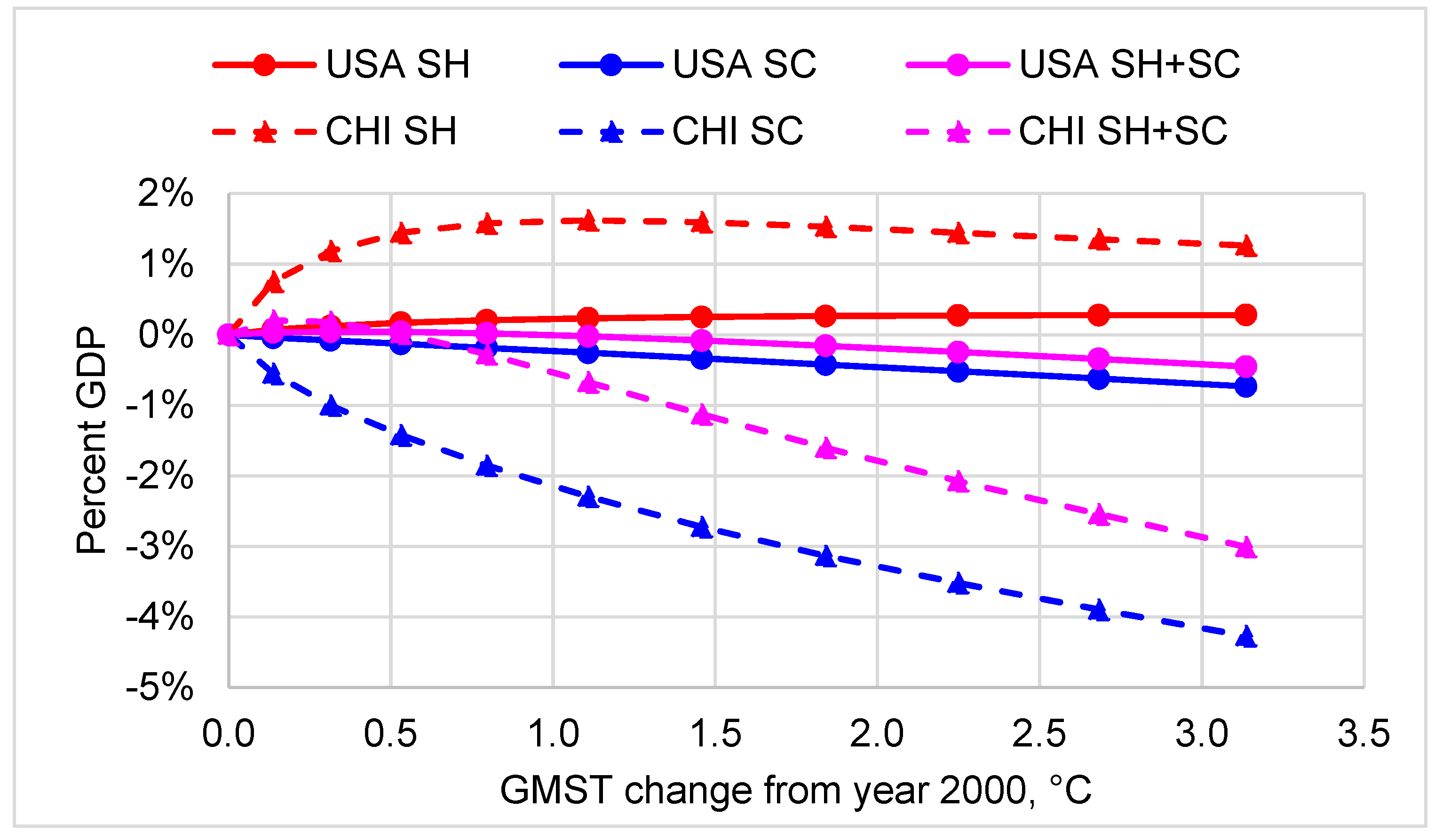
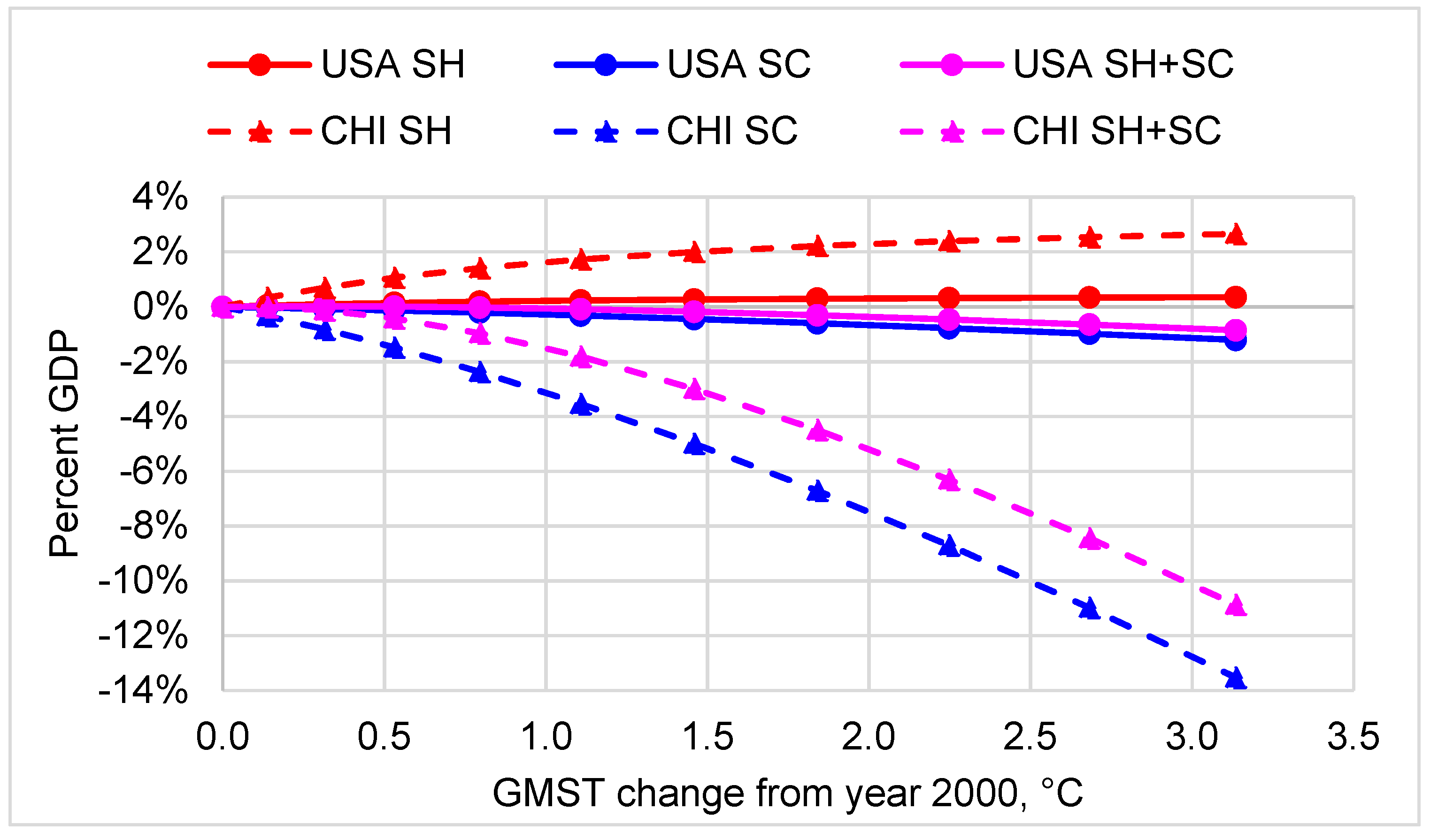
4.3. Impacts due to Non-Temperature Drivers

The proportion of the projected energy impacts due to non-temperature drivers, at +3 °C GMST change from 2000, is 37% for the USA, 75% for CHI and 67% for the World (Table 4). That is, two thirds of the projected global impacts of 3 °C global warming on energy consumption are due to non-temperature drivers. Similarly, Downing et al. [7] and Waite et al. [25] find that per capita income is a more significant driver of energy consumption change than temperature. Downing et al. [7] conclude that cooling demand is more dependent on increasing per capita income than on temperature change, whereas heating demand is relatively insensitive to increasing per capita income.
Waite et al. [25] studied urban electricity demand for heating and cooling in 18 OECD and 17 non-OECD tropical and sub-tropical cities. They found increasing energy demand as the cities become more urban, industrial and affluent. Mature urban OECD economies exhibit a cooling electricity response that is 10 to 17 times higher, per °C per capita above room temperature, than in non-OECD tropical and subtropical cities, indicating significant electricity demand growth as air conditioning is adopted. Electricity demand for heating is also increasing in subtropical areas as people are adopting electric resistance heaters. These electricity demand increases are mostly due to increasing affluence, urbanisation and industrialisation, not global warming. However, FUND regions with population centroids south of 30° N produced only 18% of global GDP in 2010, so their impact is a relatively minor contributor to the global impacts of warming.

4.4. Curvature of Heating and Cooling Demand as a Function of Temperature

Regarding the curvatures of heating and cooling demand as a function of temperature, the FUND documentation [
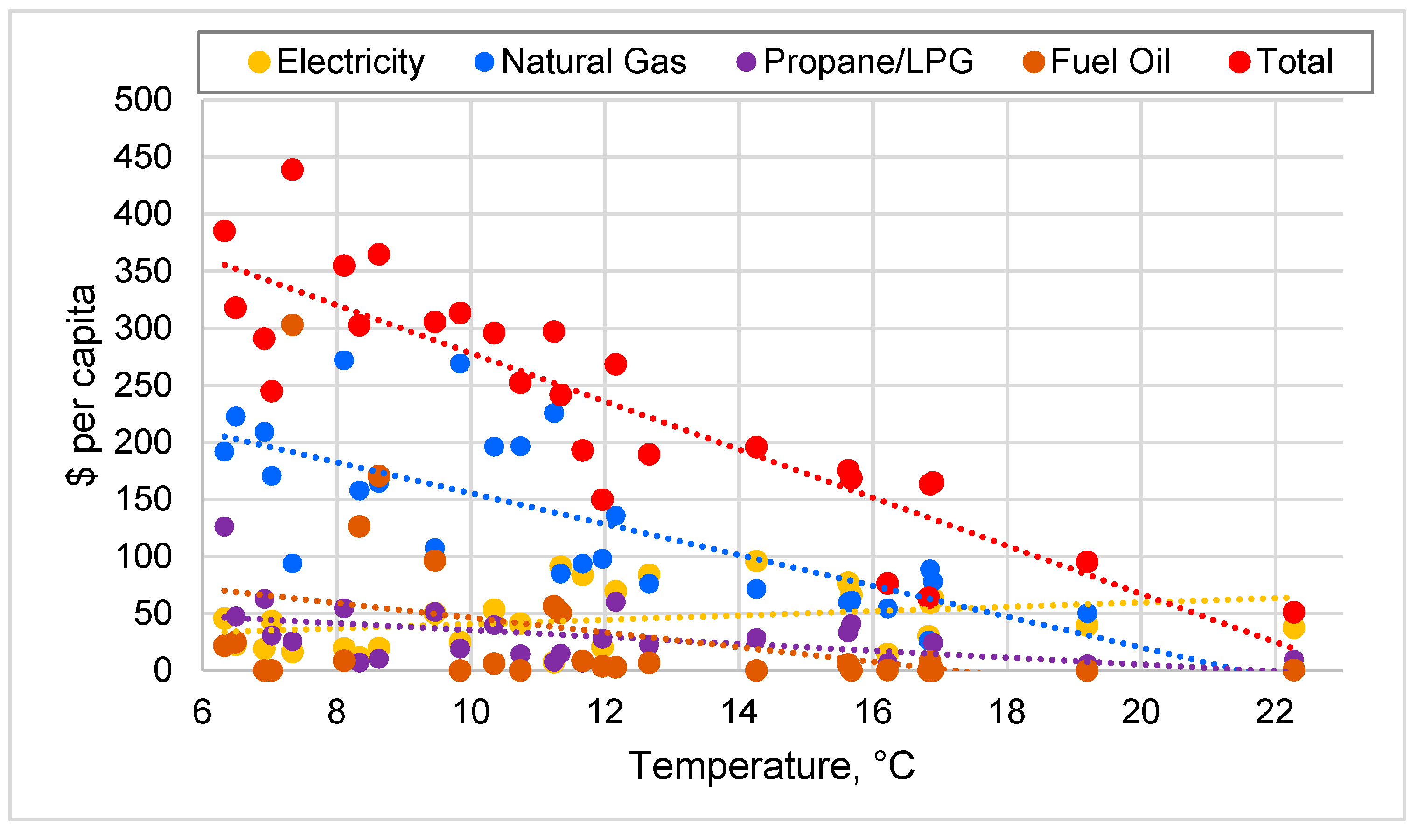
19] says that savings on heating are assumed to saturate whereas cooling is assumed to accelerate as it gets warmer. However, the EIA data show that both heating and cooling expenditure are near linear against temperature for the USA. Although the EIA data does not show the curvature over the temperature range analysed (i.e., 6 °C to 22 °C) (Section 3.1 and Appendix B), projection of the EIA data to higher temperatures indicates that heating expenditure flattens at average temperatures above 22 °C. DePaula and Mendelsohn [26] and Waite et al. [25] find that cooling expenditure will increase significantly in the tropics, but this is mostly due to increasing per capita income rather than temperature change.

4.5. Impact of Warming on Electricity Demand in Europe

A recent study indicates that the FUND energy impact functions may also be misspecified for Europe. FUND projects that the impacts of +2 °C global warming on energy consumption in WEU+EEU, with non-temperature drivers constant at 2010 values, would be –1.0% of GDP. However, consistent with our findings from the EIA data, Damm et al. [27] conclude that +2 °C global warming would reduce electricity consumption in Europe. They explain that the reduced heating electricity demand outweighs the increase in cooling demand. They studied the impact of 2 °C warming on electricity consumption in 26 European countries using a method somewhat similar to ours in that it assumes present demographic and economic structures; that is, the non-temperature drivers are constant at current levels. However, their study does not report energy expenditure or economic impact, and analyses electricity only, not the other heating energy carriers (natural gas, oil, propane, coal, biofuels, and district heat). If the other energy carriers were included, the reduction in heating expenditure, and in heating plus cooling expenditure, with increasing temperature would be greater, which means the economic impact of global warming on energy consumption in Europe would be more positive (i.e., more beneficial).

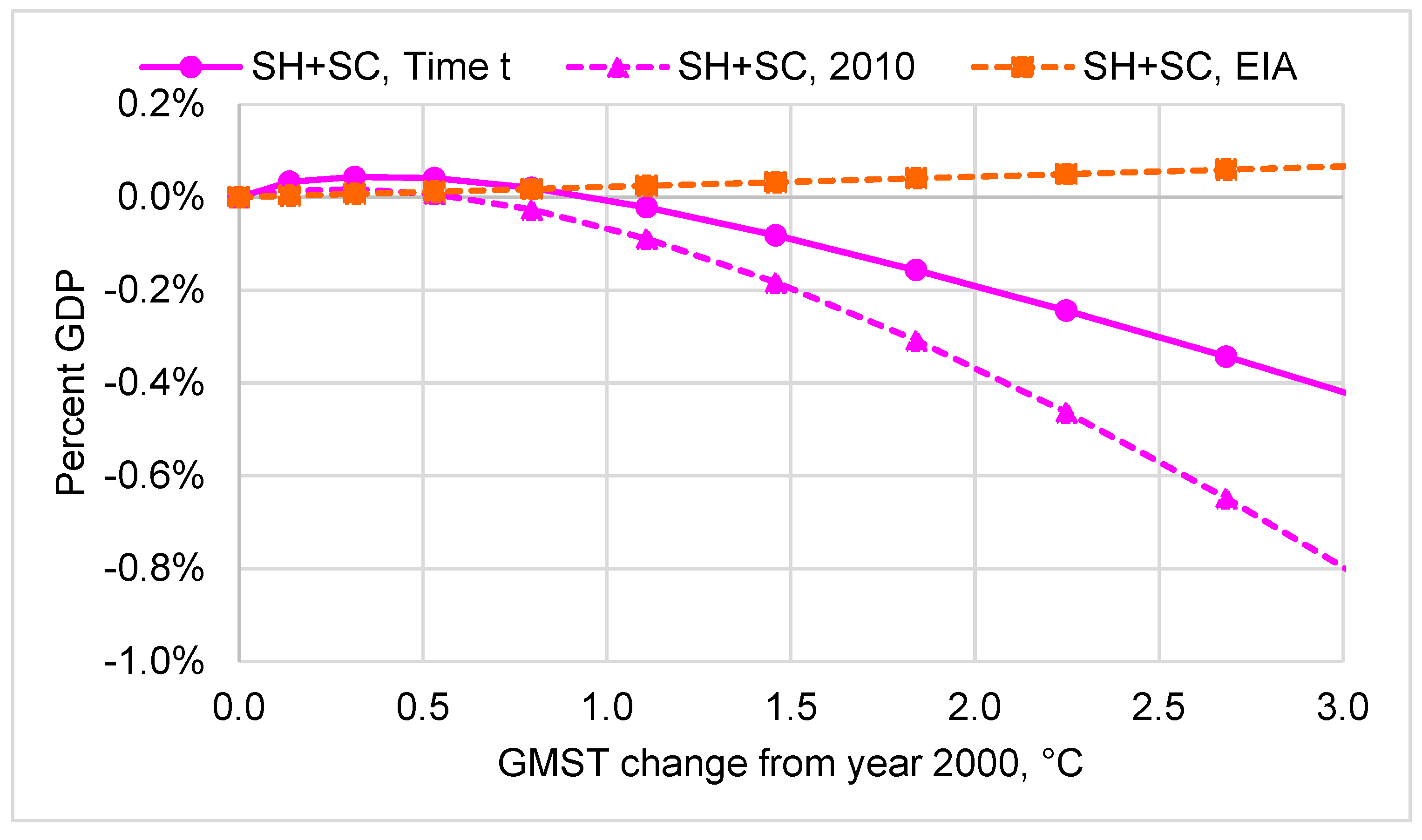
4.6. Economic Impact of Global Warming on Global Energy Consumption

We infer that the findings for USA and Europe may be indicative of the impact of global warming on the global economy because these regions span the latitudes where most of the world’s GDP is produced. In 2010, USA, WEU and EEU produced 51% of world GDP; these regions plus CHI produced 60%; FUND regions with population centroids north of 30°N produced 82% [18]. With non-temperature drivers constant at 2010 values, FUND projects the impact of +3 °C GMST to be –0.80% of GDP for the USA, –1.78% for WEU+EEU, and –10.12% for CHI. However, the EIA data indicates the impact for the USA to be +0.07%. The projected impact for WEU+EEU at +2 °C GMST is –0.99%, whereas Damm et al. find the impact of +2 °C GMST on electricity consumption in the 26 European countries would be positive. If the other heating fuels were included, the impact would be more positive. Since CHI is at similar latitude to USA and Europe, we might expect the impacts due to temperature alone might also be positive. In short, we infer from these figures that positive impacts of global warming in regions that produce 82% of world GDP are likely to exceed negative impacts in tropical countries. In this case, the impact of +3 °C GMST on energy consumption would be positive for the global economy.
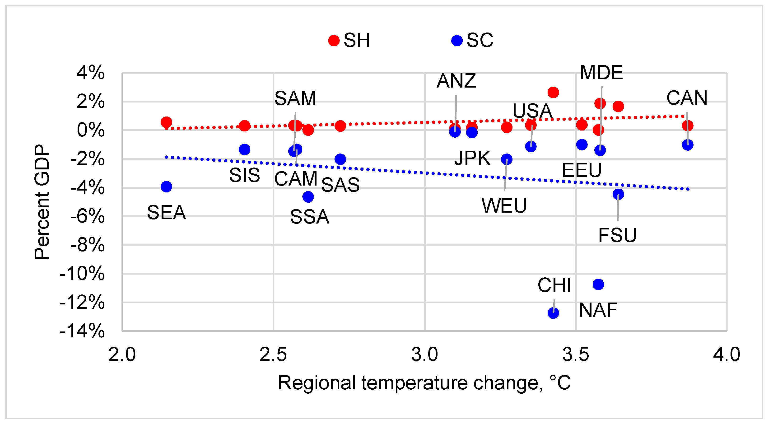
The FUND energy impact functions are the same for all regions; only parameter values vary by region. Thus the findings that the FUND projections may be pessimistic compared with the results of studies of empirical data for the USA and Europe suggest that the energy impact functions may be misspecified for other regions. For example, at +2 °C GMST with non-temperature drivers constant at 2010 values, the projected impact for WEU+EEU (–0.99%) is more negative than for the USA (–0.37%). Since WEU+EEU’s population centroid is about 10° north of USA’s (Table 3), we might expect the impacts to be more positive for WEU+EEU than for the USA. That FUND projects the opposite is another indication that the impact functions may be misspecified.

4.7. FUND3.9 Projected Global Sectoral Impacts of Warming

Figure 15 plots the global economic impacts by sector as a function of GMST change from 2000 to 2100 projected by FUND3.9 with non-temperature drivers included. The total of all impact sectors, and the total excluding energy, are also shown.
With energy impacts excluded, FUND projects the global impacts to be +0.2% of GDP at 3 °C GMST increase from year 2000. With the energy impact functions misspecifications corrected, and all other impacts are as projected, the projected total economic impact may be more positive.
The conclusion that 3 °C of global warming may be beneficial for the global economy depends, in part, on the total of the non-energy impact projections being correct, or more positive. Whether this is the case needs to be tested.

4.8. Policy Implications

The economic impact of climate policies is likely to be substantial. It is the sum of the economic impact of the policies and the cost of implementing and maintaining the policies. If global warming is beneficial, as this study indicates may be the case, then the total economic impact is the sum of the forgone benefits of the avoided global warming plus the cost of policies to mitigate warming.
Our analysis suggests that the overall impact of global warming may be positive—that is, it would increase global economic growth. If this is correct, then the positive impacts can be maximised and the negative impacts minimised by increasing wealth, but not by reducing global warming. Tol [6] concludes that the negative impacts of global warming can be reduced by reducing global warming and/or reducing poverty. However, if global warming is beneficial, then polices aimed at reducing global warming are reducing global economic growth.
According to Lomborg [28] any reductions in temperature resulting from the Paris Agreement promises would be minimal but at high cost. For example, Lomborg says that all Paris promises 2016–2030 will reduce global temperatures by just 0.05 °C in 2100, and by 0.17 °C if they continue to 2100. He estimates the most likely cost would be $1,848 billion per year in 2030. This is about 2% of projected world GDP in 2030 [20], and this estimate does not include all costs of the climate change industry.
Other studies also indicate that the cost of policies to reduce global warming is high. For example, Climate Change Business Journal [29] estimates put the climate change industry in 2013 at $1,405 billion, about 1.9% of world GDP [18,21]. Further, Insurance Journal [30], citing [29], says that the ‘climate change industry’ grew at 17–24% annually 2005–2008, 4–6% following the recession, and 15% in 2011. These growth rates are much higher than the growth rate of the world economy implying that, if they continue, which is likely with international protocols, accords and agreements such as Kyoto [31], Copenhagen [32] and Paris [1], the cost of climate policies will continue to escalate.

5. Conclusions

This study tests the validity of the FUND energy impact functions by comparing the projections against empirical space heating and space cooling energy data and temperature data for the USA. Non-temperature drivers are held constant at their 2010 values for comparison with the empirical data. The impact functions are tested at 0° to 3 °C of global warming from 2000.
The analysis finds that, contrary to the FUND projections, global warming of 3 °C relative to 2000 would reduce US energy expenditure and, therefore, would have a positive impact on US economic growth. FUND projects the economic impact to be −0.80% of GDP, whereas our analysis of the EIA data indicates the impact would be +0.07% of GDP. We infer that the impact of global warming on energy consumption may be positive for the regions that produced 82% of the world’s GDP in 2010 and, by inference, may be positive for the global economy.
The significance of these findings for climate policy is substantial. If the FUND sectoral economic impact projections, other than energy, are correct, and the projected economic impact of energy should actually be near zero or positive rather than negative, then global warming of up to around 3 °C relative to 2000, and 4 °C relative to pre-industrial times, would be economically beneficial, not detrimental.
In this case, the hypothesis that global warming would be harmful to the global economy this century may be false, and policies to reduce global warming may not be justified. Not adopting policies to reduce global warming would yield the economic benefits of warming and avoid the economic costs of those policies.
The discrepancy between the impacts projected by FUND and those found from the EIA data may be due to a substantial proportion of the impacts (37% for the US and 67% for the world) being due to non-temperature drivers, not temperature change, and to some incorrect energy impact function parameter values.
We recommend that the FUND energy impact functions be modified and recalibrated against best available empirical data. Further, we recommend that the validity of the non-energy impact functions be tested.
This study is the first to test the FUND energy impact functions against observed data for the US showing that this function overstates damages due to global warming.

Author Contributions

P.A.L. designed the research, analysed the data, and wrote the paper. K.B.G. interrogated Julia FUND3.9, analysed the data and contributed to writing the paper.

Funding

This research received no external funding.

Acknowledgments

We thank David Anthoff and Ian Cameron for assistance with using the Julia version of FUND3.9, Peter Bobroff for extracting the population centroid gridded data, Peter McCullagh for assistance with the statistical analyses, Yiyong Cai, Reza Fazeli, Brian Fisher, Warwick McKibbin, Robert Mendelsohn and Richard Tol for their reviews and suggestions, and Alan Cummine and Richard Webb for their editing of the manuscript.

Conflicts of Interest

The authors declare no conflicts of interest.

Abbreviations

°CDegree Celsius
CBECSCommercial Buildings Energy Consumption Survey
EIAUS Energy Information Administration
FUNDClimate Framework for Uncertainty, Negotiation and Distribution (FUND)
GCMGlobal Climate Model
GDPGross Domestic Product
GMSTGlobal Mean Surface Temperature
IAMIntegrated Assessment Model
NASNational Academies of Sciences, Engineering and Medicine
NOAANational Oceanic and Atmospheric Administration
NRCNational Research Council
RECSResidential Energy Consumption Survey
RTCFRegional Temperature Conversion Factor
SHSpace heating
SCSpace cooling

Appendix

Appendix A. Data Plotted in Figure 3, Figure 4, Figure 5 and Figure 7

Table A1. Space heating and space cooling per capita energy expenditure, in 2010 US$, by US state and state group, for residential consumers, and the calculated latitude and 2009 temperature of the population centroid for each.
State and State GroupsLat. °NTemp. °CRes. SH, $Res. SC, $
Massachusetts42.38.641315
CT, ME, NH, RI, VT42.57.348317
New York41.58.335729
Pennsylvania40.59.534539
New Jersey40.411.236066
Illinois41.39.824739
Michigan42.98.133813
Wisconsin43.76.529011
Indiana, Ohio40.310.427730
Missouri38.412.224559
IA, MN, ND, SD44.26.330722
Kansas, Nebraska39.510.723450
Virginia37.812.722389
Georgia33.416.9160114
Florida27.822.361211
DC, DE, MD, WV39.111.327162
North Carolina, South Carolina35.015.619290
Tennessee35.814.318781
Alabama, Kentucky, Mississippi34.615.7178118
Texas30.919.2103179
Arkansas, Louisiana, Oklahoma33.516.9160101
Colorado39.56.922510
Idaho, Montana, Utah, Wyoming42.77.018119
Arizona33.416.878203
New Mexico, Nevada36.012.014098
California35.516.27336
Alaska, Hawaii, Oregon, Washington44.511.718212
Table A2. Space heating and space cooling per capita energy expenditure, in 2010 US$, by US census division, for residential and commercial buildings, and the calculated latitude of the population centroid for each.
Census DivisionsLat. °NRes. SH, $Res. SC, $Com. SH, $Com. SC, $
New England42.44511615433
Middle Atlantic40.93544012448
East North Central41.6283277536
West North Central41.5272395933
South Atlantic33.51611284088
East South Central35.01811054653
West South Central31.71211553584
Mountain37.8153874036
Pacific37.8100303343
Table A3. Latitude and 2009 temperature at the area and population centroids, and temperature change at the population centroids at 3 °C GMST increase, by states and state groups.
US States and State GroupsArea CentroidPop. CentroidTemp. Change
°C
Lat. °NTemp. °CLat. °NTemp. °C
Massachusetts42.168.7242.278.633.48
CT, ME, NH, RI, VT44.485.7642.487.343.49
New York42.917.2241.508.343.46
Pennsylvania40.909.1140.469.463.42
New Jersey40.1111.5040.4311.243.42
Illinois40.1010.7841.299.843.45
Michigan44.846.5642.878.113.50
Wisconsin44.635.7843.726.493.52
Indiana, Ohio40.1910.4840.3510.353.42
Missouri38.3512.2238.4212.163.36
IA, MN, ND, SD45.285.5144.246.333.54
Kansas, Nebraska39.9710.3839.5210.743.40
Virginia37.5212.8937.8112.663.34
Georgia32.6317.4433.3816.853.21
Florida28.4621.7827.8222.283.04
DC, DE, MD, WV38.7611.5939.0811.343.38
North Carolina, South Carolina34.9215.7335.0515.633.26
Tennessee35.8614.2235.8114.263.28
Alabama, Kentucky, Mississippi34.0916.1134.6315.683.25
Texas31.4318.7830.9119.203.13
Arkansas, Louisiana, Oklahoma33.9716.5333.5116.903.21
Colorado38.997.3339.516.923.40
Idaho, Montana, Utah, Wyoming43.956.0542.717.033.49
Arizona34.2116.1733.3716.833.21
New Mexico, Nevada36.7711.3636.0011.963.29
California37.1514.8935.4616.223.27
Alaska, Hawaii, Oregon, Washington59.190.0644.5111.673.55
Table A4. Latitude and 2012 temperature at the area and population centroids, and temperature change at the population centroids at 3 °C GMST increase, by census division.
US Census DivisionsArea CentroidPop. CentroidTemp. Change
°C
Lat. °NTemp. °CLat. °NTemp. °C
New England44.148.0242.399.353.48
Middle Atlantic41.8410.3540.9511.033.44
East North Central42.6310.6941.5611.513.46
West North Central42.7210.7541.4711.713.46
South Atlantic33.9017.4833.4917.793.21
East South Central34.5017.0135.0416.603.26
West South Central32.4419.2731.7119.823.16
Mountain40.1410.3537.8312.103.34
Pacific55.611.7437.7515.293.34

Appendix B. Regression Results and Data Issues

A linear model provides near to the best fit over the range of latitudes and temperatures spanned by the data points for the USA; other models showed some slight improvements in fit for some regressions, but were not sufficient to warrant substituting non-linear models. Table A5 summarises the results of the regression analyses.
Table A5. Summary of the regression analyses results.
ItemDescriptionSlopeInterceptdf2-Sided p-Value
Table 3RTCF v area centroid latitude0.01010.7320141.1 ✕ 10−6
Figure 3SH, $/capita v latitude18.00–457.94259.7 ✕ 10−6
SC, $/capita v latitude−12.03529.13251.2 ✕ 10−10
Figure 4Present temp v latitude−0.9147.14257.1 ✕ 10−13
Temp at +3 °C GMST v latitude−0.8849.33251.5 ✕ 10−12
Figure 5SH, $/capita v present temp−18.88460.48254.5 ✕ 10−6
SC, $/capita v present temp11.96−76.57252.1 ✕ 10−9
Figure 6SH, $/capita v temp change−19.040.00
SC, $/capita v temp change12.720.00
SH+SC, $/capita v temp change−6.320.00
Figure 7Res. SH, $/capita v present temp23.54−664.4271.3 ✕ 10−2
Res. SC, $/capita v present temp−12.18532.9471.5 ✕ 10−4
Com. SH, $/capita v present temp7.77−228.1273.5 ✕ 10−2
Com SC, $/capita v present temp−4.76231.2072.4 ✕ 10−3
Figure 8Res. SH, $/capita v temp change−19.040.00
Res. SC, $/capita v temp change12.720.00
Com. SH, $/capita v temp change−9.100.00
Com. SC, $/capita v temp change5.570.00
Res + Com SH, $/capita v temp change−28.140.00
Res + Com SC, $/capita v temp change18.290.00
Res + Com SH+SC, $/cap v temp change−9.840.00
Figure 10SH+SC, %GDP v temp change−0.0079−0.0006
Figure 11SH, %GDP v temp change0.0050−0.0096
SC, %GDP v temp change−0.01290.0090
Figure 14SH, EIA $/capita v temp change−28.140.00
SC, EIA $/capita v temp change18.290.00
SH+SC, EIA $/capita v temp change−9.840.00
SH, FUND $/capita v temp change−42.91−26.81
SC, FUND $/capita v temp change240.18−265.56
SH+SC, FUND $/capita v temp change197.27−292.37
The slopes of the linear regressions of the residential expenditure data (Figure 3, Figure 4 and Figure 5) are statistically significant at the 1% level, and of the commercial buildings data (Figure 7) for cooling at the 1% level and for heating at the 5% level. The negative intercepts for heating in Figure 3, Figure 5 and Figure 7, and the $0 expenditure for cooling below 6.4 °C, are discussed in Section 3.4.
The regression results in Figure 10 and Figure 11 are not used in any calculations; the trendlines are shown on the charts for illustrative purposes.
The linear regression results in Table A5 for the FUND projections in Figure 14 are close fits to the data points. However, the best fit models are non-linear. The equations are:
SH: y = 2.9556x2 − 62.625x + 5.8652
SC: y = 87.719x1.5
SH+SC: y = 20.985x2 + 57.302x − 60.377
where: y is $/capita, and x is temperature change.

Appendix B.1. Explanation of Increasing Residuals with Decreasing Temperature

Figure 5 and Figure 7 show that the absolute value of the heating residuals increases as temperature decreases. Causes include climate effects (relatively colder winters and nights in continental and mountain climates than in coastal climates, at similar average temperature), and differences in proportions and prices of fuels (electricity, natural gas, propane/LPG, and heating oil) used for heating in different states.
Figure A1 plots residential per capita heating expenditure by fuel and 2009 average temperature, by state and state group, sorted by temperature. Expenditure is at 2009 state average fuel prices.
Figure A1. Residential per capita heating expenditure by fuel, and 2009 temperature, by state and state group.
Energies 12 03575 g0a1
Figure A2 plots residential per capita heating expenditure by fuel against 2009 temperature. Expenditure is calculated as consumption times fuel prices at US average price per fuel. This removes the effect of different fuel prices in the different states.
Figure A2. Residential per capita heating expenditure, at state fuel prices, against temperature.
Energies 12 03575 g0a2
We test the magnitude of the effects of different fuel proportions and prices by:
  • substituting natural gas prices for propane/LPG and fuel oil prices—this removes the effect of different proportions of these fuels being used in different states.
  • substituting US average prices per fuel for state prices—this removes the effect of fuel price differences between states.
The test results are numbered 1 to 4 in Table A6. The projections with non-temperature drivers at 2010 values, and the impacts calculated from the expenditure data, and summarised in Table 2, are included for comparison.
Table A6. Comparison of the effect of different fuel consumption proportions and fuel prices in different states on the economic impact of 3 °C GMST increase, relative to 2000, on US space heating and space cooling energy expenditure. The projections are included for comparison.
Expenditure Data Sources and CalculationsExpenditure Change (US $bn)
HeatingCoolingTotal
Projections, relative to 2000 (Table 2)‒53.09174.87121.79
Results from EIA data (Table 2)−28.97 18.84 −10.14
1. Consumption times fuel prices, fuels at state prices−28.86 18.84 −10.02
2. All fuels at US average prices−29.83 20.79 −9.04
3. Propane/LPG and heating oil at state natural gas prices−23.91 18.84 −5.08
4. Electricity at US average price, propane/LPG and heating oil at US average natural gas price−23.90 20.79 −3.12
Expenditure Data Sources and CalculationsEconomic Impact (% GDP)
HeatingCoolingTotal
Projections, relative to 2000 (Table 2)0.35%−1.14%−0.80%
Results from EIA data (Table 2)0.19%−0.12%0.07%
1. Consumption times fuel prices, fuels at state prices0.19%−0.12%0.07%
2. All fuels at US average prices0.19%−0.14%0.06%
3. Propane/LPG and heating oil at state natural gas prices0.16%−0.12%0.03%
4. Electricity at US average price, propane/LPG and heating oil at US average natural gas price0.16%−0.14%0.02%
The total impacts calculated using the different fuel consumption proportions and prices are opposite in sign to the projections. The differences between the projected impacts and those calculated from the EIA data range from US $125–$132 billion.

Appendix B.2. Data Deficiencies

There are deficiencies in the EIA consumption and fuel price data, which we have attempted to compensate for by our calculations.
  • Some fuel price and consumption data are not included in the EIA data tables. We have compensated by infilling missing data by differences and proportions from the available data.
  • There are as few as one significant figure for some consumption data for some fuels in some states, state groups and divisions, which increases uncertainty. We have partly compensated by using EIA fuel prices per physical units, which have more significant figures.
Fuel prices for commercial buildings are not provided by use category, such as for heating and cooling. The prices are the average per fuel for all uses, including water heating, refrigeration, computers, etc. The actual prices of fuels for heating and cooling (electricity, natural gas, fuel oil and district heat) may be higher or lower than the average.
The commercial buildings expenditures may be understated because the fuel prices are full-year averages, which are generally below the winter prices for heating fuels and the summer prices for cooling energy (electricity).
The residential expenditures for tests 1 to 4 in Table A6 are also calculated from fuel prices and consumption data, which are incomplete; we have partly compensated as we have done for the commercial buildings data.

Appendix B.3. Other Sources of Uncertainty

A source of uncertainty in the US energy expenditure versus temperature analyses is the RTCF at the population centroid of each US state. We do not have these data. We therefore estimated the RTCF at the population centroids by applying the slope of RTCF of the world regions against their area centroid latitudes to the difference between the area and population centroid latitudes of each US state and census division. Residential impacts at +3 °C GMST differ by 27% for heating and −2% for cooling when calculated by state and state group or by census division. We interpret this as being due to differences between the slope of RTCF against latitude for US states and census divisions compared with the slope of RTCF versus latitude for the 16 world regions. The difference may also be due to differences between the slopes for different states and census divisions within the USA.
Another potential source of uncertainty is the temperature at the population centroid of each state. We estimated these by applying the slope of temperature against area centroid latitudes of all US states to the difference in latitude of the area and population centroids of each state. This assumes the same slope applies to all states, which ignores influences such as distance from oceans and large water bodies, altitude, etc. The residential data is for year 2009, and the commercial data is for year 2012. Average temperatures were marginally higher in 2012 than in 2009, and fuel prices were different, thus, adding uncertainty to the calculated impacts of residential plus commercial buildings.

Appendix C. Notes

[I]
The method used for analysing the EIA data is explained below.
First, we find relationships between temperature and per capita expenditure for heating and cooling. The steps are:
1.
Calculate per capita heating and cooling energy expenditure by state for large states and by groups of smaller states (27 in total) for residential buildings [14], and by US census division (9 in total) for both residential [14] and commercial buildings [15]. Expenditures are converted to 2010 US dollars [21].
2.
Get the area and the area centroid latitude [23], and the population and the population centroid latitude [24], of each state. Calculate the latitude of the area centroid and population centroid of each state group and each census division.
3.
Regress per capita energy expenditure per state and state group (for residential) and per census division (for commercial) against the population centroid latitudes.
4.
Get the 2009 and 2012 average temperature for each state [22]. Calculate the area-weighted temperature for each state group and census division. Regress temperature against area centroid latitude per state and state group, and per census division.
5.
Apply the slopes to convert the temperatures at the area centroid latitudes to the temperatures at the population centroid latitudes.
6.
Regress per capita expenditure against temperature at the population centroid latitudes.
Next, we estimate the impact of a 3°C GMST increase, relative to year 2000, on per capita expenditure, total US expenditure, and the economic impact in percent of US GDP. The steps are:
  •  
7.
Regress the regional temperature conversion factor (RTCF) of the world regions (FUND3.9 Tables, Table RT [19]) against their area centroid latitudes. Apply the slope to calculate the RTCF at the population centroid latitude, and the temperature change at 3°C GMST increase, for each US state, state group and census division.
8.
Calculate per capita expenditure versus temperature change at the population centroid latitudes, at 3°C GMST increase.
9.
Calculate per capita expenditure change at the population centroid latitudes, at 3°C GMST increase.
10.
Convert per capita expenditure change to total US expenditure change ($ billions), and to the economic impact as a percent of 2010 US GDP.
[II]
Regional temperature is derived by multiplying GMST by the regional temperature conversion factor (RTCF). “The RTCFs for each region were derived from the spatial climate change pattern averaged over 14 GCMs” [19]
[III]
The steps to convert the temperature change at the area centroid latitude to that at the population centroid latitude of the world regions, and to calculate the energy sector impacts for each region at 3°C GMST increase, are:
  • Calculate the latitude of the area centroid [33,34] and population centroid [35,36] for each region.
  • Regress the RTCFs (FUND3.9 Tables, Table RT [19]) of the 16 regions against their area centroid latitudes. Apply the slope to calculate the RTCF at the population centroid latitude of each region.
  • Calculate the temperature change at each region’s population centroid at 3°C GMST increase.
  • Get the FUND3.9 projected heating and cooling impacts for each region at 3°C GMST increase.
  • Regress the heating and cooling impacts for each region against the temperature change at its population centroid latitude.
[IV]
The high data point at latitude 44.5°N is state group ‘Alaska, Hawaii, Oregon and Washington’; it is high due to moderation of temperatures caused by the oceanic influence. The low data point at latitude 39.5°N is Colorado; it is low due to its relatively high elevation compared with other states at similar latitude.
[V]
Note that Figure 8 is in units of expenditure change per capita, whereas Figure 10 and Figure 11 are in units of percent of GDP; positive expenditure change has a negative impact on GDP.
[VI]
Impacts due to non-temperature drivers are impacts at time t minus impacts with non-temperature drivers at 2010 values.
[VII]
α is a parameter that relates temperature change to heating/cooling expenditure.
[VIII]
The projected US impacts at latitudes 30°, 35°, 40°, 45° north are calculated as follows:
  • Calculate the RTCF for each latitude by multiplying the latitude by the regression slope of the 16 FUND world regions.
  • Modify the α parameters for heating and cooling at each latitude by multiplying the αUSA by a factor that accounts for the temperature difference between the USA area centroid latitude (44.97°N) and each latitude. For example, at 30°N latitude for the USA:
    α(heat)30 = α(heat)USA*atan(T1990*RTCF30)/atan(T1990*RTCFUSA)
    α(cool)30 = α(cool)USA*(T1990 * RTCF30)β/(T1990*RTCFUSA)β
  • Calculate the impacts at each latitude using the corresponding α values and the heating and cooling impact equations.

References

  1. The United Nations Framework Convention on Climate Change (UNFCCC). The Paris Agreement. Available online: http://unfccc.int/process-and-meetings/the-paris-agreement/the-paris-agreement (accessed on 3 April 2018).
  2. Kolstad, C.; Urama, K.; Broome, J.; Bruvoll, A.; Cariño-Olvera, M.; Fullerton, D.; Gollier, C.; Hanemann, W.M.; Hassan, R.; Jotzo, F. Social, economic and ethical concepts and methods. In Climate Change 2014: Mitigation of Climate Change; Edenhofer, O., Pichs-Madruga, R., Sokona, Y., Farahani, E., Kadner, S., Seyboth, K., Adler, A., Baum, I., Minx, J.C., Eds.; Cambridge University Press: Cambridge, UK; New York, NY, USA, 2014; pp. 173–248. Available online: https://www.ipcc.ch/site/assets/uploads/2018/02/ipcc_wg3_ar5_chapter3.pdf (accessed on 29 December 2018).
  3. National Academies of Sciences Engineering and Medicine. Valuing Climate Damages: Updating Estimation of the Social Cost of Carbon Dioxide; The National Academies Press: Washington, DC, USA, 2017; p. 280. Available online: https://www.nap.edu/catalog/24651/valuing-climate-damages-updating-estimation-of-the-social-cost-of (accessed on 26 April 2018).
  4. Anthoff, D.; Tol, R.S.J. FUND - Climate Framework for Uncertainty, Negotiation and Distribution, 3.9. 2014. Available online: http://www.fund-model.org (accessed on 3 April 2018).
  5. Pindyck, R.S. Climate change policy: What do the models tell us? J. Econ. Lit. 2013, 51, 860–872. Available online: https://www.aeaweb.org/articles?id=10.1257/jel.51.3.860 (accessed on 26 January 2019). [CrossRef]
  6. Tol, R.S.J. The Economic Impacts of Climate Change. Rev. Environ. Econ. Policy 2018, 12, 4–25. Available online: http://dx.doi.org/10.1093/reep/rex027 (accessed on 26 April 2018). [CrossRef] [Green Version]
  7. Downing, T.E.; Eyre, N.; Greener, R.; Blackwell, D. Full Fuel Cycle Study: Evaluation of the Global Warming Externality for Fossil Fuel Cycles with and without CO2 Abatement and for Two Reference Scenarios; Environmental Change Unit, University of Oxford: Oxford, UK, 1996; Available online: http://www.fund-model.org/files/DowningEtAl1996b.pdf (accessed on 3 November 2017).
  8. Downing, T.; Eyre, N.; Greener, R.; Blackwell, D. Projected costs of climate change for two reference scenarios and fossil fuel cycles. In Report to the European Commission, Project ExternE, Environmental Change Unit, Oxford; Downing, T., Eyre, N., Greener, R., Blackwell, D., Eds.; Environmental Change Unit, University of Oxford: Oxford, UK, 1996; Available online: http://www.fund-model.org/files/DowningEtAl1996a.pdf (accessed on 3 November 2017).
  9. Hodgson, D.; Miller, K. Modelling UK energy demand. In Global Warming and Energy Demand; Barker, T., Ekins, P., Johnstone, N., Eds.; Routledge: London, UK, 1995; pp. 172–187. Available online: https://www.amazon.com/Global-Warming-Energy-Demand-Environmental/dp/0415109809 (accessed on 3 November 2017).
  10. Bonen, A.; Semmler, W.; Klasen, S. Economic Damages from Climate Change: A Review of Modeling Approaches. In Schwartz Center for Economic Policy Analysis, The New School, Working Paper; Bonen, A., Semmler, W., Klasen, S., Eds.; SCEPA: New York, NY, USA, 2014; Volume 3, p. 60. Available online: http://www.economicpolicyresearch.org/resource-library/research/economic-damages-from-climate-change-a-review-of-modeling-approaches (accessed on 26 April 2018).
  11. National Research Council. Hidden Costs of Energy: Unpriced Consequences of Energy Production and Use; National Academies Press: Washington, DC, USA, 2010; Available online: https://www.nap.edu/download/12794 (accessed on 3 April 2018).
  12. Tol, R.S.J. The economic impact of climate change in the 20th and 21st centuries. Clim. Chang. 2013, 117, 795–808. Available online: https://doi.org/10.1007/s10584-012-0613-3 (accessed on 3 April 2018). [CrossRef]
  13. Tol, R.S.J. The Economic Impact of Climate Change in the 20th Century, 1st ed.; Harvard Dataverse: Cambridge, MA, USA, 2011; Available online: https://dataverse.harvard.edu/dataset.xhtml?persistentId=hdl:1902.1/15573 (accessed on 4 March 2018).
  14. Energy Information Administration (EIA). Residential Energy Consumption Survey (RECS), 2009 RECS Survey Data, Consumption and Expenditures, by End Uses by Fuel. Available online: https://www.eia.gov/consumption/residential/data/2009/index.php?view=consumption#end-use (accessed on 3 April 2018).
  15. Energy Information Administration (EIA). Commercial Buildings Energy Consumption Survey (CBECS), 2012 CBECS Survey Data, Consumption & Expenditures. Available online: https://www.eia.gov/consumption/commercial/data/2012/index.php?view=consumption (accessed on 2 August 2018).
  16. Ürge-Vorsatz, D.; Cabeza, L.F.; Serrano, S.; Barreneche, C.; Petrichenko, K. Heating and cooling energy trends and drivers in buildings. Renew. Sustain. Energy Rev. 2015, 41, 85–98. Available online: https://www.sciencedirect.com/science/article/pii/S1364032114007151 (accessed on 3 April 2018). [CrossRef] [Green Version]
  17. Serrano, S.; Ürge-Vorsatz, D.; Barreneche, C.; Palacios, A.; Cabeza, L.F. Heating and cooling energy trends and drivers in Europe. Energy 2017, 119, 425–434. Available online: https://www.sciencedirect.com/science/article/pii/S0360544216318874 (accessed on 30 June 2018). [CrossRef] [Green Version]
  18. World Bank. GDP (Constant 2010 US$). Available online: https://data.worldbank.org/indicator/NY.GDP.MKTP.KD (accessed on 24 April 2019).
  19. Anthoff, D.; Tol, R.S.J. FUND-Versions. 3.9. 2014. Available online: http://www.fund-model.org/versions (accessed on 3 April 2018).
  20. Anthoff, D.; Tol, R.S.J. FUND3.9 Julia Version; 3.9. GitHub: San Francisco, CA, USA, 2018. Available online: https://github.com/fund-model/MimiFUND.jl (accessed on 5 January 2018).
  21. World Bank. GDP Deflator. Available online: https://data.worldbank.org/indicator/NY.GDP.DEFL.ZS?locations=US (accessed on 5 April 2018).
  22. NOAA National Centers for Environmental Information. Climate at a Glance: National Time Series, Average Temperature. Available online: http://www.ncdc.noaa.gov/cag/ (accessed on 9 February 2018).
  23. US Census Bureau. State Area Measurements and Internal Point Coordinates. Available online: https://www.census.gov/geographies/reference-files/2010/geo/state-area.html (accessed on 3 April 2018).
  24. US Census Bureau. Centers of Population. 2010. Available online: https://www.census.gov/geographies/reference-files/2010/geo/2010-centers-population.html (accessed on 3 April 2018).
  25. Waite, M.; Cohen, E.; Torbey, H.; Piccirilli, M.; Tian, Y.; Modi, V. Global trends in urban electricity demands for cooling and heating. Energy 2017, 127, 786–802. Available online: https://www.sciencedirect.com/science/article/abs/pii/S0360544217304784 (accessed on 16 February 2019). [CrossRef] [Green Version]
  26. DePaula, G.; Mendelsohn, R. Development and the impact of climate change on energy demand: Evidence from Brazil. Clim. Chang. Econ. 2010, 1, 187–208. Available online: https://www.worldscientific.com/doi/abs/10.1142/S2010007810000157 (accessed on 5 November 2018). [CrossRef]
  27. Damm, A.; Köberl, J.; Prettenthaler, F.; Rogler, N.; Töglhofer, C. Impacts of+ 2 C global warming on electricity demand in Europe. Clim. Serv. 2017, 7, 12–30. Available online: https://www.sciencedirect.com/science/article/pii/S2405880716300012 (accessed on 26 April 2019). [CrossRef]
  28. Lomborg, B. The impact and cost of the 2015 Paris Climate Summit, with special focus on US policies. In The House of Representatives Committee on Science, Space and Technology, 114th Congress, First Session; Lomborg, B., Ed.; USA Government Publishing Office: Washington, DC, USA, 2015; pp. 98–118. Available online: https://www.govinfo.gov/content/pkg/CHRG-114hhrg97771/pdf/CHRG-114hhrg97771.pdf (accessed on 26 April 2019).
  29. Ferrier, G. The Climate Change Industry, EBI Report 4000; Climate Change Business Journal: San Diego, CA, USA, 2015; Available online: https://ebionline.org/product/report-4000-the-climate-change-industry/ (accessed on 26 April 2019).
  30. Jergler, D. Is Climate Change Now Its Own Industry? In Climate Control; Jergler, D., Ed.; Insurance Journal: San Diego, CA, USA, 2015; Available online: https://www.insurancejournal.com/news/national/2015/07/30/377086.htm (accessed on 3 April 2019).
  31. The United Nations Framework Convention on Climate Change (UNFCCC). The Kyoto Protocol. Available online: https://unfccc.int/process-and-meetings/the-kyoto-protocol/what-is-the-kyoto-protocol/what-is-the-kyoto-protocol (accessed on 18 April 2019).
  32. The United Nations Framework Convention on Climate Change (UNFCCC). The Copenhagen Accord. Available online: https://unfccc.int/process-and-meetings/conferences/past-conferences/copenhagen-climate-change-conference-december-2009/copenhagen-climate-change-conference-december-2009 (accessed on 18 April 2019).
  33. Central Intelligence Agency. The World Factbook 2016–17. Available online: https://www.cia.gov/library/publications/the-world-factbook/fields/277.html (accessed on 5 August 2019).
  34. World Bank. Land Area (Sq Km), All Countries and Economies. Available online: https://data.worldbank.org/indicator/AG.LND.TOTL.K2 (accessed on 17 February 2018).
  35. Center for International Earth Science Information Network-CIESIN-Columbia University. Gridded Population of the World, Version 4 (GPWv4): Population Count, Revision 10; NASA Socioeconomic Data and Applications Center (SEDAC): Palisades, NY, USA, 2017; Available online: https://doi.org/10.7927/H4PG1PPM (accessed on 26 April 2019).
  36. World Bank. Population, Total, All Countries and Economies. Available online: https://data.worldbank.org/indicator/SP.POP.TOTL (accessed on 17 February 2018).
Figure 1. “The global average sectoral economic impact of climate change in the 20th and 21st century as functions of time (top panel) and temperature (bottom panel)” [12]. Total is of all impact sectors. Total* is of all impact sectors from 1900 to 2000, and of all sectors except energy from 2000 to 2100. (Adapted from Figure 3 in Tol [12] by permission from Springer Nature).
Energies 12 03575 g001
Figure 2. FUND regions. (Source: FUND Home [4]).
Energies 12 03575 g002
Figure 4. Average temperature versus population centroid latitude of the US states and state groups at Present (2009), at 3 °C GMST increase, and the temperature change [IV].
Energies 12 03575 g004
Figure 5. Residential per capita space heating and space cooling expenditure versus temperature at the population centroid, for the 27 states and state groups.
Energies 12 03575 g005
Figure 6. Residential per capita space heating and space cooling expenditure change versus temperature change at 3 °C GMST increase, for the 27 states and state groups.
Energies 12 03575 g006
Figure 7. Residential and commercial buildings per capita space heating and space cooling expenditure versus population centroid latitude, for the nine census divisions.
Energies 12 03575 g007
Figure 8. Residential and commercial buildings per capita space heating and space cooling expenditure change versus temperature change at 3 °C GMST increase for the nine census divisions.
Energies 12 03575 g008
Figure 9. Economic impact of US energy expenditure as functions of GMST change, relative to 2000. Pink solid line is the Julia FUND3.9 projection. Pink dashed line is the projection with non-temperature drivers constant at 2010 values. The orange dashed line is from the EIA data.
Energies 12 03575 g009
Figure 10. Economic impact of 3 °C GMST increase on energy expenditure for FUND regions plotted against temperature change at the population centroid latitude.
Energies 12 03575 g010
Figure 11. Data points in Figure 10 separated into space heating and space cooling components
Energies 12 03575 g011
Figure 12. USA and CHI, heating, cooling and heating plus cooling economic impact (percent of GDP) versus GMST change from 2000, with non-temperature drivers a function of time.
Energies 12 03575 g012
Figure 13. USA and CHI heating, cooling and heating plus cooling economic impact (percent of GDP) versus GMST change from 2000, with non-temperature drivers constant at 2010 values.
Energies 12 03575 g013
Figure 14. Impact of 3 °C GMST increase on US space heating and space cooling per capita energy expenditure versus temperature change at latitude 30°N to 45°N from the analysis of the EIA data, and from projections with non-temperature drivers at 2010 values.
Energies 12 03575 g014
Figure 15. FUND3.9 projected global sectoral economic impact of climate change as a function of GMST change from 2000. Total* is of all impact sectors except energy.
Energies 12 03575 g015
Table 1. Impact of a 3 °C GMST increase on US annual space heating and space cooling expenditure, 2010 US$ billion (negative values are savings).
ItemUnitsRes. SHRes. SCCom. SHCom. SCTotal
Residential & Commercial$ bn–19.60 13.10 –9.37 5.74 –10.14
Table 2. Economic impact of 3 °C GMST increase, from 2000, on US space heating and space cooling energy expenditure in residential and commercial buildings. Projections are with non-temperature drivers constant at 2010 values.
ItemUnitsHeatingCoolingTotal
US GDP, 2010US$ bn 15,318.74
SH + SC expenditure, FUND projectionUS$ bn–53.09174.87121.79
SH + SC expenditure, EIA dataUS$ bn–28.97 18.84 –10.14
GDP %, FUND projection% GDP0.35%–1.14%–0.80%
GDP %, EIA data% GDP0.19%–0.12%0.07%
Table 3. Area and population RTCFs, their latitudes, and temperature change at the population centroid latitude at 3 °C GMST increase, by region.
RegionCodeRTCF at Area
Centroid
Centroid Latitude (°)RTCF at Pop.
Centroid
Temp.
Change (°C)
AreaPop.
USAUSA1.194144.9737.361.11733.35
CanadaCAN1.471264.3146.391.29023.87
Western EuropeWEU1.124851.3247.941.09073.27
Japan and South KoreaJPK1.055536.2135.881.05223.16
Australia and New ZealandANZ0.9676–27.46–33.991.03353.10
Central and Eastern EuropeEEU1.167647.1947.771.17353.52
Former Soviet UnionFSU1.286656.8049.581.21363.64
Middle EastMDE1.154628.4932.351.19363.58
Central AmericaCAM0.880420.9918.870.85902.58
South AmericaSAM0.8504–13.30–13.860.85612.57
South AsiaSAS0.907423.6323.610.90712.72
Southeast AsiaSEA0.70985.496.030.71522.15
China PlusCHI1.184736.5632.331.14203.43
North AfricaNAF1.143027.2532.071.19173.57
Sub-Saharan AfricaSSA0.87801.480.860.87172.62
Small Island StatesSIS0.75179.9214.850.80152.40
Table 4. Proportions of projected impacts that are due to temperature change at +3 °C GMST from 2000, and to non-temperature drivers over the same time period.
Cause of ImpactsSHSCSH+SC
USA:
Temperature change41%54%63%
Non-temp drivers59%46%37%
CHI:
Temperature change15%22%25%
Non-temp drivers85%78%75%
World:
Temperature change20%29%33%
Non-temp drivers80%71%67%
Table 5. USA and CHI economic impact (in percent of GDP) of heating and cooling at 3 °C GMST increase from 2000, for two scenarios: non-temperature drivers are 1) a function of time, and 2) at 2010 values. Bottom rows are possible causative factors: ratio of change in per capita income from 2000, and parameters α (heat) and α (cool). The CHI/USA ratio is in the last column.
Scenario and Possible Causative FactorsUSCHICHI/US
Non-temperature drivers as a function of time:
SH, Time t0.28%1.29%4.6
SC, Time t–0.70%–4.16%6.0
SH+SC, Time t–0.42%–2.87%6.9
Non-temperature drivers at 2010 values:
SH, 20100.35%2.63%7.6
SC, 2010–1.14%–12.75%11.2
SH+SC, 2010–0.80%–10.12%12.7
Possible causative factors:
Per capita income change (ratio)3.6517.054.7
α (heat)0.004290.039719.3
α (cool)–0.00212–0.0289113.6

