Mitigation Strategy for Duck Curve in High Photovoltaic Penetration Power System Using Concentrating Solar Power Station

Abstract

Concentrating solar power (CSP) station is counted as a promising flexible power supply when the net load power curve is duck-shaped in high photovoltaic (PV) penetration power system, which may lead to the serious phenomenon of PV curtailment and a large-capacity power shortage. This paper presents a mitigation strategy that replaces thermal power station with CSP station to participate in the optimal operation of power system for solving the duck-shaped net load power curve problem. The proposed strategy utilizes the dispatchability of thermal storage system (TSS) and the fast output regulation of unit in the CSP station. Simultaneously, considering the operation constraints of CSP station and network security constraints of the system, an optimization model is developed to minimize the overall cost including operation and penalty. The results obtained by nonlinear optimization function demonstrate that the replacement of concentrating solar power (CSP) station contributes to reducing the PV curtailment and lost load, while increasing the available equivalent slope for power balance. Thus, the proposed mitigation strategy can promote the penetration of PV generation and improve the flexibility of power system.

1. Introduction

Photovoltaic (PV) power generation is the mainstream of solar power generation due to the reduction of PV modules’ raw material cost and policy support [1,2,3]. However, the output curve of PV power generation is a semi-envelope shape with a single midday peak due to its intermittence and fluctuation [4]. Its variation trend does not match with the typical daily load curve with double peak in terms of time, resulting in the net load curve resembling duck silhouette that is known as duck curve [5]. The total load power curve minus the renewable energy generation curve is defined as the duck curve [6]. The concept of duck curve is intended to graphically depict the problem of excessive generation during the midday and insufficient supply for rapid ramp in a short time at sunset in the conventional power system. The duck curve problem will result in curtailment of PV power largely and imbalance between power supplies and load demand seriously, threatening the safe and stable operation of power system [7,8].

Currently, the mitigation strategy for solving duck curve problem is primarily carried out from two aspects: mining the potential of demand-side response and improving the flexibility of power generation side.

With the application of smart meters, smart appliances, such as air conditioners and water heaters, can aggregate the response potential to narrow down the peak-valley difference of load for reducing the slope of ramping [9,10,11]. Such measures are mainly applied for load centers with substantial distributed PV. While the scenario considered in this paper is the large-scale renewable energy delivery area where there’re few schedulable demand responses, so the second aspect is the major consideration.

At present, the main approaches of increasing power generation side flexibility include: (1) Retrofit conventional thermal power stations (TPS). In [12], the renovation of TPSs changed its minimum generation requirements to eliminate PV curtailment at noon. An automatic load gain control strategy based on condensate throttling facilitated the TPSs’ load following performance for ramp need [13]. (2) Control the real-time orientation of solar panels flexibly. This approach makes the PV output grid-friendly but increases the amount of PV curtailment [14]. (3) Deploy flexible power supplies. Pumped-storage stations and gas turbines have been widely utilized in conjunction with renewable energy station to reduce the fluctuation of its power integrated [15,16]. Additionally, as a representative of the burgeoning power supply technologies, the deployment of energy storage device can time-shift the load demand to turn the duck curve into a straight line [17].

However, in our scenario, such as Gansu province, China, it deploys numerous PV power stations without matched hydro-power and gas resources. Meanwhile, due to the economic factor, grid-side energy storage cannot be configured on a large scale [18]. Concentrating solar power (CSP) generation technology is another emerging controllable solar power generation technology, which has the superior regulation capability to regulate output more accurately and quickly by equipping thermal storage system (TSS) with a certain capacity [19]. The development of CSP generation technology provides a new thought to mitigate the impacts of duck curve on power system. Therefore, the CSP station with better regulation capability should be dispatched to mitigate the duck curve problem. It can form a multi-energy complementary system with PV power stations or wind power stations to improve the accommodation of renewable energy [20,21]. Furthermore, the CSP station equipped with TSS has technical and economic competitiveness due to the lower investment cost of thermal storage technology parallel with the mainstream electric energy storage technology, so it can also time-shift peak load strategically by storing thermal energy during the day and generating electricity at sunset [22]. Extensive researches on the modeling and application of CSP generation technology have been done, the regulation capability of which is considered to provide a beneficial support function in the future high renewable energy penetrated power system [23,24]. Generally, the CSP model can be divided into two categories according to different application scenarios: (1) Dynamic model. Based on the modeling of differential equations, its time scale can be accurate to the level of seconds, which is mainly applied to imitate the real-time operating condition of CSP station for transient fault analysis [25]. (2) Static model. Based on the modeling of steady-state difference equations, its time scale can only reach the hour level, which is suitable for developing the economic optimal dispatching strategies of the CSP station participating in the power system operation [26]. From the research emphasis of this paper, the static model is more applicable for analyzing the day-ahead optimal dispatching operation of power system including CSP station.

CSP station needs to consider two points to solve the duck curve problem: (1) the risk of over-generation in the duck belly at noon and (2) the ramp need in the duck neck at sunset. Hence, this paper develops an optimization model of the power system including the CSP stations considering its operation modes, exploiting the TSS’s dispatch-ability for accommodating surplus solar energy during the midday and utilizing the unit’s fast output regulation for providing sufficient ramp rate during the sunset.

The major contributions of this paper lie in threefold:

(1)

Develop the simplified static energy flow model for CSP station based on its internal structure, deriving its operation modes and providing constraints for the subsequent optimization model.

(2)

Propose a mitigation strategy to improve the flexibility of the grid for increasing the available equivalent slope, which utilizes the different operation modes of the CSP station and replaces the conventional TPS with the same capacity CSP station.

(3)

Establish an optimization model to ensure the reliability of power supply and reduce amount of PV curtailment by taking economic optimization as the goal and considering the operation constraints of CSP station and the network security constraints of power system.

The rest of the paper is organized as follows: Section 2 analyses the modeling approach of CSP station and its operation mode. Section 3 proposes the mitigation strategy for duck curve using CSP station based on the discussion of cause analysis of duck curve formation. Section 4 establishes the optimization model of mitigation strategy including optimization objectives and constraints. Case study and conclusions are outlined in Section 5 and Section 6 respectively.

2. Modeling and Operation Mode of CSP Station

Based on the operation mechanism of the CSP station, this section presents the mathematical model of CSP station appropriate for solving duck curve, and analyzes the two operation modes of the CSP station with the thermal storage system (TSS) and its fast regulation capability of the unit, laying a foundation for the establishment of the optimization model in the next section.

2.1. CSP Model

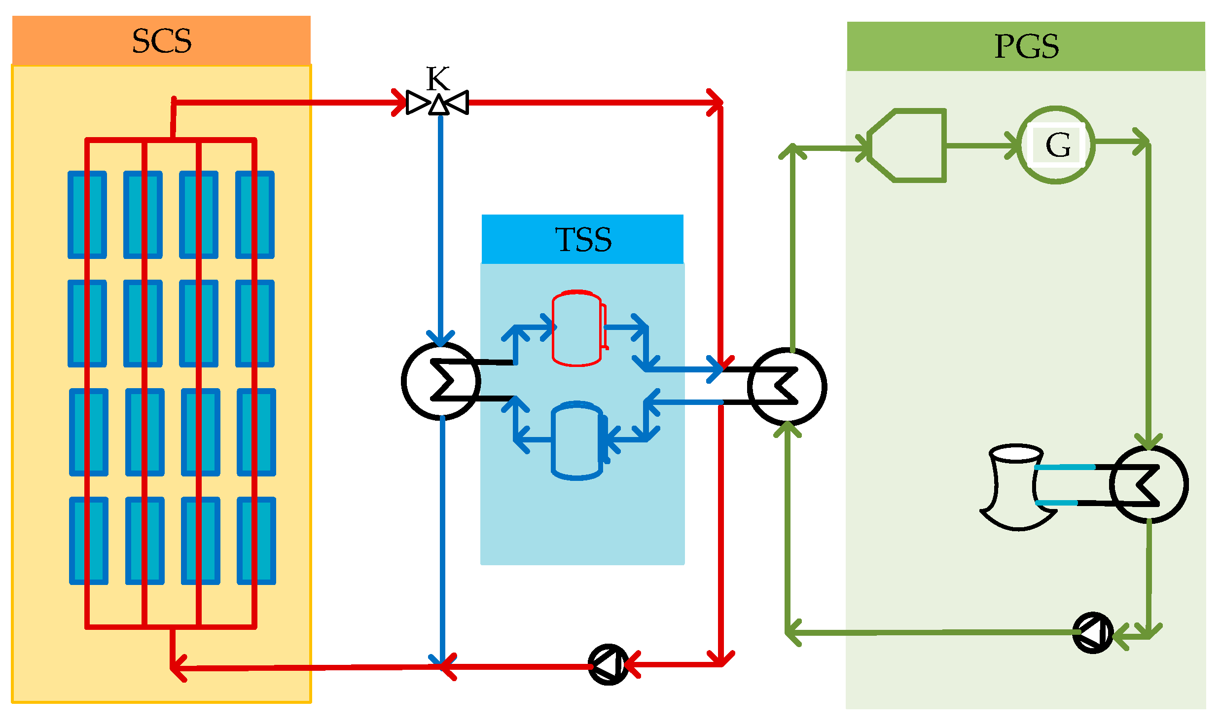
The structure of the CSP station with TSS proposed is described in Figure 1.

Generally, the CSP station is composed of three subsystems, namely, solar concentrator system (SCS), TSS and power generation system (PGS) [19]. Solar energy is concentrated by the plane mirrors and converted into thermal energy in the SCS. Thermal energy then acts on the high-pressure water passing into the SCS, generating superheated steam with high temperature and pressure after preheating, evaporation and overheating. When the CSP station operates in different modes, the superheated steam from the SCS flows to different paths. In this paper, there are two circulation schemes for superheated steam taken into consideration: (1) First, the superheated steam directly flows through valve K to drive steam turbine G for generating electricity. (2) The second scheme is that when the superheated steam flows through the valve K, it also enters the TSS to store excess thermal. After reaching the rated capacity of the TSS, it releases thermal to drives the steam turbine together with the superheated steam according to the dispatching instruction [27]. For the TSS, it includes high temperature thermal storage tank and low temperature thermal storage tank. Therefore, superheated steam can be stored at different levels according to the degree of overheating. High superheated steam is stored by high temperature thermal storage tank, while slightly superheated steam is stored by low temperature thermal storage tank. The PGS consists of a series of thermodynamic elements, the chief of which is the steam turbine, which generates electricity by using superheated steam transmitted from the first two subsystems.

For day-ahead optimal operation of the power system including CSP station, the mathematical model of CSP station should focus on describing the exchange of energy flow to develop the steady state equation only up to hour level. The dynamic differential processes of thermal flow and temperature accurate to second time scale can be ignored. Based on the above operation mechanism of CSP station, its structure can be simplified to the form shown in Figure 2.

According to Figure 2, the flowchart of developing simplified operation model of CSP station is depicted in Figure 3, which can be divided into four parts, namely SCS, HTF, TSS, and PGS.

(1) The thermal power $P_t^{S-H}$ released by the SCS can be obtained by the direct normal irradiance of solar $D_t$ from weather station and the relevant data of CSP station including solar field’s area $S_{SF}$ solar-thermal conversion efficiency ${\eta }_{SF}$ and thermal exchange efficiency ${\eta }_{SH}$, as follows:

$$P_t^{S-H}={\eta }_{SH}{\eta }_{SF}{S}_{SF}{D}_t$$

(1)

(2) Regarding the energy transmission and conversion hub, HTF, as a node, the power balance equation inside the CSP station can be obtained as follows if there is thermal exchange process between HTF and TSS:

$$P_t^{S-H}+P_t^{T-H}=P_t^{H-T}+P_t^{H-P}$$

(2)

where $P_t^{S-H}$, $P_t^{T-H}$ are the thermal power absorbed by the HTF from the SCS and the TSS, and $P_t^{H-T}$, $P_t^{H-P}$ are the thermal power released by the HTF to the TSS and the PGS.

(3) The thermal storage and release process of the TSS has operation efficiency, and cannot be carried out at the same time, which has upper and lower limits in the single process. Therefore, the thermal storage and release constraints of the TSS are:

$$P_t^{ch}={\eta }_c{P}_t^{H-T}$$

(3)

$$P_t^{dis}=P_t^{T-H}/{\eta }_d$$

(4)

$$P_t^{ch}{P}_t^{dis}=0$$

(5)

$$0\le P_t^{ch}\le P^{ch,\max }$$

(6)

$$0\le P_t^{dis}\le P^{dis,\max }$$

(7)

where $P_t^{ch}$, $P_t^{dis}$ are the actual thermal storage and release power of the TSS, ${\eta }_c$, ${\eta }_d$ are the thermal storage and release efficiency of the TSS and $P^{ch,\max }$, $P^{dis,\max }$ are the maximum thermal storage and release power of the TSS.

Simultaneously, the TSS has capacity constraints, and thermal storage and release can only be carried out between the upper and lower limits of capacity.

$$E_t-P_t^{dis}\Delta t\ge E_{down}$$

(8)

$$E_t+P_t^{ch}\Delta t\le E_{up}$$

(9)

where $E_t$ is the capacity state of the TSS at time t and $E_{up}$, $E_{down}$ are the upper and lower limits of the TSS capacity. The maximum thermal storage capacity of TSS is usually expressed as full load hours (FLH) [28]. For example, 8FLHs indicate that the maximum thermal storage of the TSS can enable the CSP station to operate at maximum output power for 8 hours without solar energy. Then:

$$E_{up}={\rho }_{\mathrm{TSS}}{P}_{\max }^{csp}$$

(10)

where ${\rho }_{\mathrm{TSS}}$ is the number of hours in FLH and $P_{\max }^{csp}$ is the maximum output of CSP station.

(4) The output electric power $P_t^{csp}$ of the PGS can be expressed as a function of the input thermal power:

$$P_t^{csp}=f(P_t^{H-P})$$

(11)

The operation constraint and ramping constraint of the steam turbine unit of the CSP station can be expressed as:

$$P^{csp,\min }\le P_t^{csp}\le P^{csp,\max }$$

(12)

$$-R^{csp.d}\le P_t^{csp}-P_{t-1}^{csp}\le R^{csp,u}$$

(13)

where, $P^{csp,\max }$, $P^{csp,\min }$, $R^{csp,u}$ and $R^{csp,d}$ are the upper and lower limit of the output power and the up and down ramp rate of the CSP station’s unit, respectively.

2.2. Operation Mode of CSP Station

According to the Equation (1), the power balance among the SCS, TSS and PGS in the CSP station depends on the dynamic balance between $P_t^{S-H}$, $P_t^{T-H}$, $P_t^{H-T}$ and $P_t^{H-P}$, and when the circulation schemes of $P_t^{S-H}$ are different, the operation mode of the CSP station is also different. There’re mainly two operation modes which is determined by the condition of sunlight and the strategy of dispatch for the CSP station:

(1) Direct power generation (DPG) mode: Electricity is generated directly without the TSS process of thermal storage and release. That means the power balance Equation (1) turns into:

$$\{\begin{array}{c}{P}_t^{S-H}=P_t^{H-P}\\ P_t^{T-H}=0\\ P_t^{H-T}=0\end{array}$$

(14)

(2) TSS mode: Electricity is generated by SCS and TSS, and TSS stores thermal energy from surplus solar energy. That means the power balance Equation (1) is the same as before.

For DPG mode, it converts solar energy into electricity in real time, lacking the performance for load regulation. TSS mode can store excess solar energy at noon in the form of thermal using TSS, and release thermal from the TSS to provide the ramp slope required for the power shortage when the PV decreases suddenly at sunset. But the amount of energy stored and released depends on the capacity of the TSS.

2.3. The Regulation Capability of the Units

This paper mainly evaluates the regulation capability of the units from the point of the maximum power that can be raised or lowered at a certain time [29]. As shown in Equations (15) and (16), the maximum power raised or lowered at a certain time is generally limited by the factors of the unit’s minimum operating output, maximum operating output and ramp rate. For the units of different types of power stations, the corresponding restriction factors mentioned above are not the same, so the regulation capability of the units is also different.

$$P_t^{up}=\min \{(P^{\max }-P_t),R^{up}\cdot \Delta t\}$$

(15)

$$P_t^{down}=\min \{(P_t-P^{\min }),R^{down}\cdot \Delta t\}$$

(16)

where $P_t^{up}$, $P_t^{down}$ represent the unit’s power that can be raised or lowered at time t; $P^{\max }$, $P^{\min }$ represent the unit’s maximum and minimum operating output; $R^{up}$, $R^{down}$ represent the unit’s ramp rate; $P_t$ represent the unit’s actual operating output at time t and $\Delta t$ is the time interval. As described in Figure 4, when the difference between the unit’s actual operating output at time t and its maximum or minimum operating output is less than the unit’s ramp rate in $\Delta t$ time interval, the unit is adjusted according to the difference, that is, according to the blue line in Figure 4. On the contrary, the unit is adjusted according to the ramp rate, that is, according to the red line in Figure 4.

The output of conventional thermal power units can only adjust the installed capacity by 2–5% per minute, limited by the delay and inertia of steam turbine valve opening and closing [12]. The regulation capability is not enough to cope with the power shortage of fast ramping due to the duck curve. Nevertheless, the CSP station fundamentally supports the output regulation of the unit through the thermal exchange system, which can be controlled well. Therefore, the unit of the CSP station can be adjusted by 20% installed capacity per minute at the soonest [28].

3. Mitigation Strategy for Duck Curve Using CSP Station

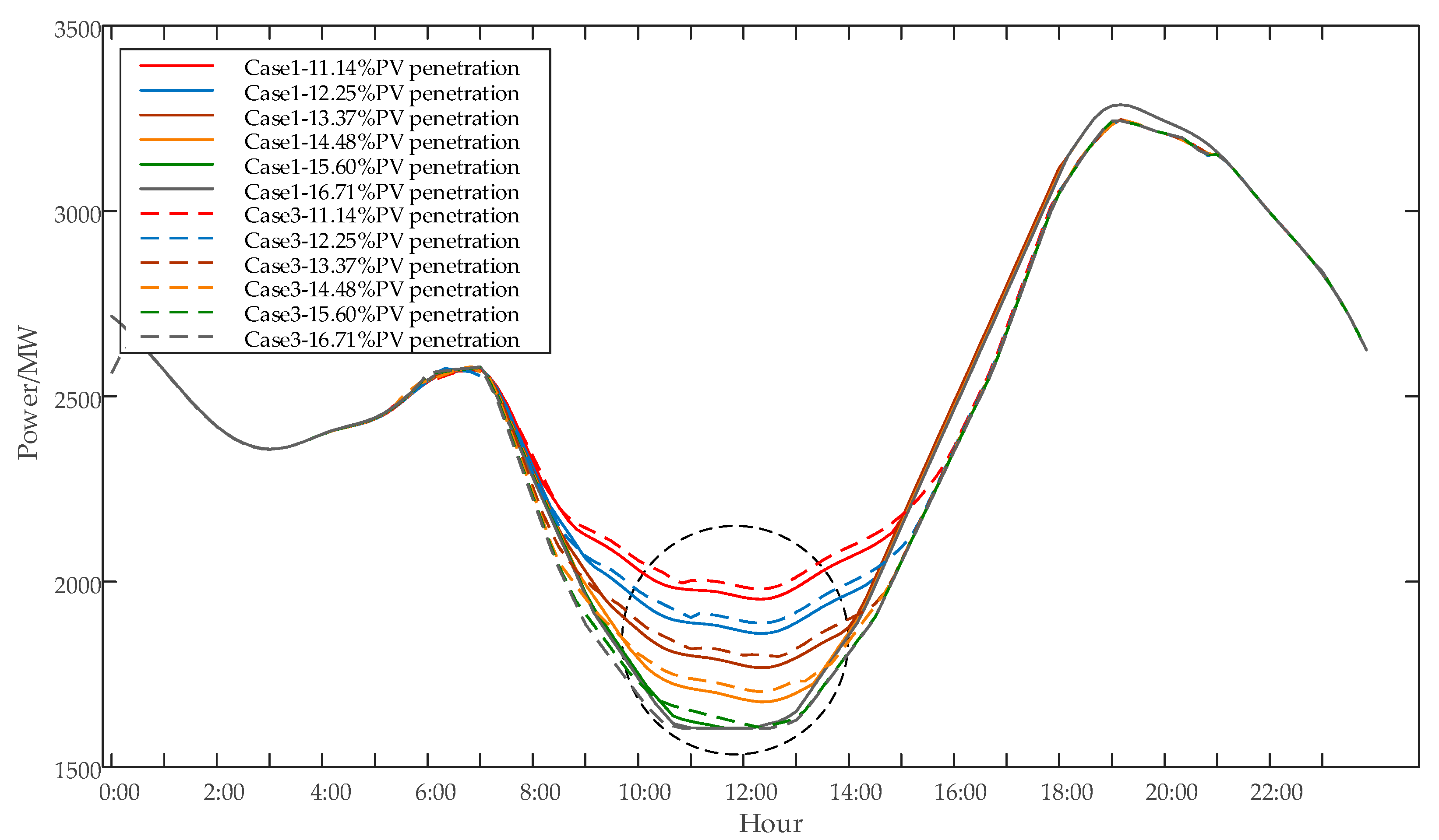
With the increase of PV penetration, the duck-shaped net load power curve will become obvious gradually, as described in Figure 5 [30]. The calculation method of the PV penetration percentages in this paper is carried out referred to the literature [31], which means the percentage of the total output of all PV power stations taking up the total load power in the system, as shown in Equation (17):

$$P{V}_{pentration}=\frac{{\displaystyle \sum _{t=1}^T{\displaystyle \sum _{i=1}^{N_{pv}}{P}_{i,t}^{pv}}}}{{\displaystyle \sum _{t=1}^T{\displaystyle \sum _{i=1}^{N_{losd}}{P}_{i,t}^{load}}}}\times 100\%$$

(17)

where $P{V}_{pentration}$ represents the penetration of PV; $P_{i,t}^{pv}$ is the output power of the ith PV power station at time t, $P_{i,t}^{load}$ is the demand power of the ith load node at time t; N_pv, N_load represent the number of PV power stations and load node, and T is the total operating time.

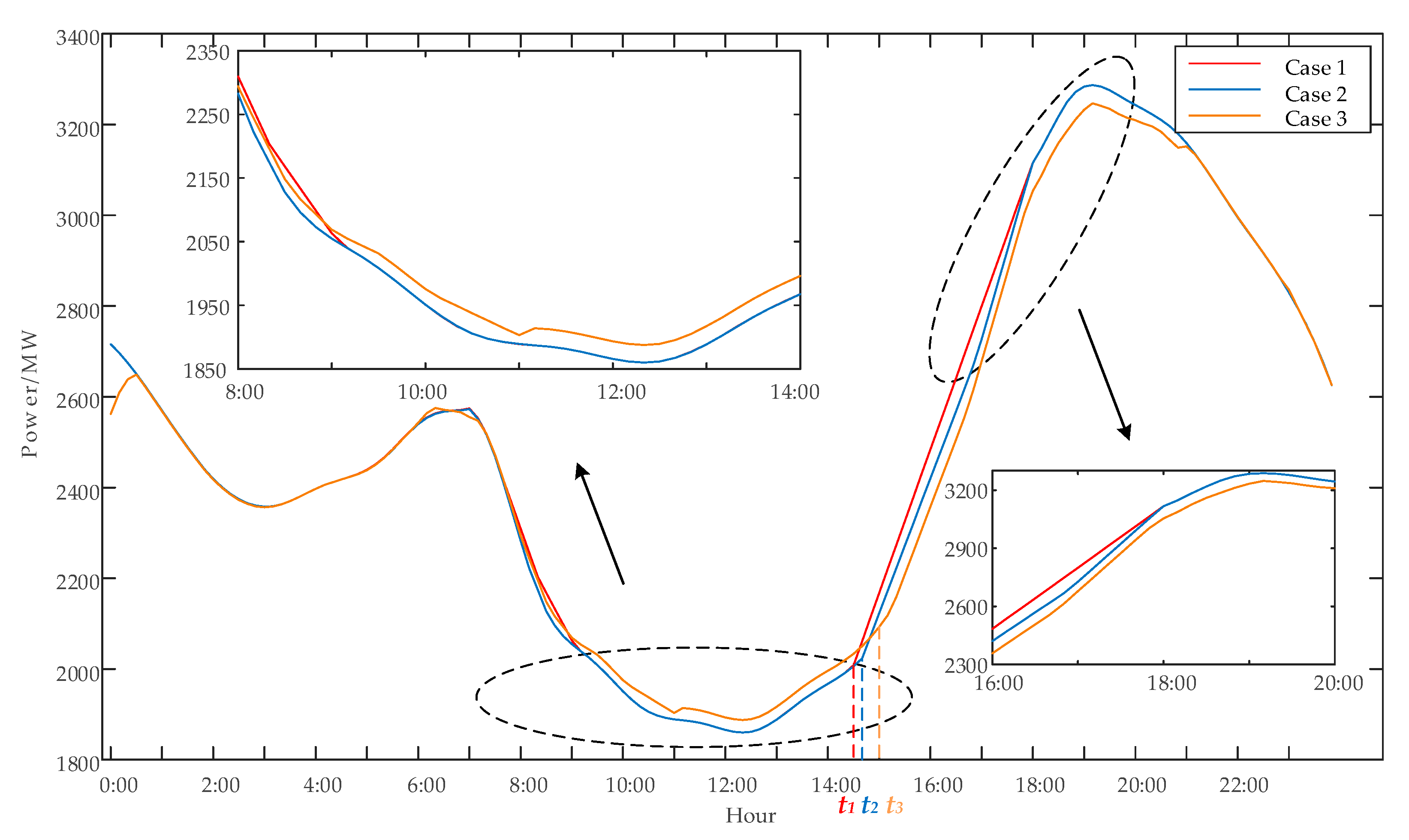
The fluctuation of duck curve should be met by the active power of other power supplies in the power system immediately. During the decreasing segment of the duck abdomen, the traditional power supplies need to reduce its output promptly to cope with the stage of abundant PV generation at noon, avoiding the risk of over-generation. During the increasing segment of the duck neck, traditional power supplies inversely need to increase output rapidly at sunset to make up for the fast loss of PV power, meeting the demand of evening peak load. However, it is difficult for the regulation capability of conventional power system to support the demand of fast ramping down and up during the segment of the duck abdomen and duck neck. According to the study of the regulation capability, the CSP station can adjust output power more quickly. Meanwhile, when the TSS operates in TSS mode, the CSP station can time shift the load power. Therefore, the main idea of mitigation strategy for duck curve using CSP station is described in Figure 6.

4. Optimization Model

4.1. Objective Function

According to the idea of Figure 7, the schematic diagram of the optimization model is depicted as follows, that is, the net load power obtained by subtracting the PV predicted power from the load predicted power is optimally allocated to the CSP station with TSS and TPS, considering the lost load and PV curtailment.

Considering the operation cost of various power stations in the system and the penalty cost of PV curtailment and lost load, the formula for the objective function is as follows:

$$\{\begin{array}{c}{\displaystyle \sum _{t=1}^T{\displaystyle \sum _{i=1}^{N_{th}}(a_i^{th}{P}_{i,t}^{th}{}^2+b_i^{th}{P}_{i,t}^{th}}}+c_i^{th})+\\ {\displaystyle \sum _{t=1}^T{\displaystyle \sum _{i=1}^{N_{csp}}(a_i^{csp}{P}_{i,t}^{csp}+a_i^{TES}(P_{i,t}^{ch}+}}{P}_{i,t}^{dis}))+\\ {\displaystyle \sum _{t=1}^T{\displaystyle \sum _{i=1}^{N_{pv}}(a_i^{pv}{P}_{i,t}^{lp})}}+{\displaystyle \sum _{t=1}^T{\displaystyle \sum _{i=1}^{N_{losd}}(a_i^{load}{P}_{i,t}^{ll}}})\end{array}$$

(18)

The first line in the Equation (18) is the operating cost of TPSs. Where $a_i^{th}$, $b_i^{th}$ and $c_i^{th}$ are the output cost coefficient of the ith TPS and $P_{i,t}^{th}$ is the output power of the ith TPS at time t. The output coefficients represent the multinomial coefficients of the quadratic polynomial operation cost function of thermal power stations. The second is the operating cost of the CSP station. Where $a_i^{csp}$ is the output cost coefficient of the ith CSP station and $P_{i,t}^{csp}$ is the output power of the ith CSP station at time t. $a_i^{TES}$ is the output cost coefficient of the TSS and $P_{i,t}^{ch}$, $P_{i,t}^{dis}$ are the actual thermal storage and release power of the TSS in the ith CSP station at time t. N_th, N_csp represent the number of TPSs and CSP stations. The third is the penalty costs of PV curtailment and lost load. Where $a_i^{pv}$ is the penalty coefficient of PV curtailment in the ith PV power station, $P_{i,t}^{lp}$ is the curtailment power of the ith PV power station at time t, $a_i^{load}$ is the penalty coefficient of lost load in the ith load node and $P_{i,t}^{ll}$ is the lost power of the ith load node at time t.

4.2. Constraints

(1) Operation Constraints of CSP Station

The operation constraints of CSP station are Equations (1)–(14) in Section 2.1.

(2) Network Security Constraints

Considering active power balance constraint, line power equation constraint, line transmission power limit constraint and node phase angle constraint, the system network security constraints formulas in this paper are derived sequentially:

$${\displaystyle \sum _{i=1}^{N_{th}}{P}_{i,t}^{th}+{\displaystyle \sum _{i=1}^{N_{csp}}{P}_{i,t}^{csp}}}+{\displaystyle \sum _{i=1}^{N_{pv}}(P_{i,t}^{pv}-P_{i,t}^{lp})}={\displaystyle \sum _{i=1}^{N_{load}}(P_{i,t}^{load}-P_{i,t}^{ll})}$$

(19)

$$P_{ij,t}=B_{ij}({\theta }_{i,t}-{\theta }_{j,t})$$

(20)

$$-P_{ij,\max }\le P_{ij,t}\le P_{ij,\max }$$

(21)

$$-\pi \le {\theta }_{i,t}\le \pi$$

(22)

where $P_{ij,t}$ is the transmission power of the line between node i and node j at time t, $B_{ij}$, $P_{ij,\max }$ are the susceptance and the thermal stability limit of the line ij respectively, and ${\theta }_{i,t}$, ${\theta }_{j,t}$ are the phase angle of the node i and node j at time t.

(3) Unit Capacity and Ramp Constraint

$$P_i^{th,\min }\le P_{i,t}^{th}\le P_i^{th,\max }$$

(23)

$$-R_i^{th,d}\Delta t\le P_{i,t}^{th}-P_{i,t-1}^{th}\le R_i^{th,u}\Delta t$$

(24)

Equations (23) and (24) are the capacity and ramp constraint of the steam turbine unit in the TPS. The form is the same as Equations (12) and (13), but the parameters are different. Where $P_i^{th,\min }$, $P_i^{th,\max }$ are the upper and lower limit of the capacity in the ith TPS, and $R_i^{th,d}$, $R_i^{th,u}$ are the ascending and descending ramp, respectively, whose units are MW/min.

(4) PV Curtailment Constraint

$$0\le P_{i,t}^{lp}\le P_{i,t}^{pv}$$

(25)

That is, the curtailment power of the ith PV power station cannot be greater than its output power at time t.

(5) Lost Load Constraint

$$0\le P_{i,t}^{ll}\le P_{i,t}^{load}$$

(26)

That is, the lost power of the ith load node is less than its demand power at time t.

5. Case Study

5.1. Simulation Settings

The mitigation strategy was verified on the modified IEEE-24 node system, as shown in Figure 8. The nodes connecting the generators are the TPSs, except that the node 16 is replaced by CSP station with the same capacity later. Additionally, the operating power of node 18 and 21 keeps constant in the optimization process. The PV power station is located in the node 19. The PV and load prediction power on three typical days, namely, the spring equinox (or autumn equinox), summer solstice and winter solstice, in Gansu province of China is selected as the reference data of PV power station and total load in this paper, as described in Figure 9 respectively.

This paper adopts contrastive analysis:

Case 1: Only an aggregated PV power station is connected to node 19. Therefore, the number of variables to be optimized is 99.

Case 2: Based on case 1, the TPS in node 16 is replaced by the CSP station with the same capacity and the CSP station operates in DPG mode. Therefore, the number of variables to be optimized is increased to 100.

Case 3 (strategy proposed in this paper): Based on case 2, but the CSP station operates in TSS mode. Therefore, the number of variables to be optimized is increased to 103, adding the thermal charging and discharging output data and capacity data of TSS.

The output power range of the TPSs in the simulation system is shown in

Table 1. The output power range of the thermal power stations (TPS) units.

Node Number	Minimum Operating Output (MW)	Maximum Operating Output (MW)
1	62.4	192
2	62.4	192
7	75	300
13	207	591
15	66.3	215
16	54.3	155
22	60	300
23	248.6	660

, and the output cost coefficients a, b and c standing for $a_i^{th}$, $b_i^{th}$ and $c_i^{th}$ are described in

Table 2. The output cost coefficients of the TPS units.

Node Number	a ($/MW2)	b ($/MW)	c ($)
1	0	130	400.6849
2	0.014142	16.0811	212.3076
7	0.052672	43.6615	781.521
13	0.00717	48.5804	832.7575
15	0.328412	56.564	86.3852
16	0.008342	12.3883	382.2391
22	0	0.001	0.001
23	0.008342	12.3883	382.2391

. The ramp rate of TPS unit is set as the maximum operating output that can be adjusted by 2% per minute. The output cost coefficient of the TSS in the CSP station is 5 $/MW and the lower limits of the TSS capacity are set as 10% of the maximum capacity. The output cost coefficient of the CSP station’s unit is 21.53 $/MW, and the ramp rate are set as 15.5 MW/min, i.e., adjust 10% of the maximum operating output per minute. The penalty cost coefficients of PV curtailment and lost load are 11 $/MW and 1000 $/MW respectively.

The computing platform is configured with Inter(R) Core (TM) i3-4170 central processing unit and 8G memory capacity. The computing software is MATPOWER v7.0b1 based on MATLAB optimization toolbox, FMINCON function.

5.2. Simulation Results

5.2.1. Analysis of the Effectiveness of the Proposed Strategy

Taking the predicted power of PV power station and total load in Figure 9a as the basic data to increase the PV integrated proportions, the changes of the overall cost, PV curtailment power and lost load power of the three cases at the same PV penetration are respectively described in Figure 10.

Additionally, the output power curves of all generators in case 1 and case 3 at different PV penetration are shown in Figure 11.

With the increase of PV penetration, the difference between the output power curves of case 1 and case 3 will gradually decrease. Meanwhile, the output power of all generators at noon circled by the dotted line will not change, which states that the phenomenon of over-generation occurs again. Even if the proposed strategy is adopted, the power balance of power system can only be maintained by PV curtailment under the circumstances. Combined with the changing trend of lost load in Figure 10, when the PV penetration is 15.60% or above, the lost load of case 1 reaches the maximum of 0.2029 MW, and there is no change thereafter. It indicates that 15.60% has reached the maximum PV penetration. Similarly, the maximum PV penetration of case 3 is 25.62%, suggesting that the proposed strategy can improve the maximum PV penetration of the system on the premise of guaranteeing the power supply reliability of the system. However, only when the PV penetration is less than the maximum can the effectiveness of the proposed strategy be demonstrated.

5.2.2. Analysis of the Net Load Power Curve Change

When different cases are adopted at the same PV penetration, taking 12.25% as an example, the output curve of all generators in the simulation system, namely the net load power curve, is shown in Figure 12. According to Figure 5, the emergency ramp need occurs between 16:00 and 21:00. This paper uses the trapezoidal integral method to calculate the ramp need of duck curve between 16:00 and 21:00 on three typical days and the available equivalent slope of three cases between 16:00 and 21:00, as shown in

Table 3. Comparison of ramp need on three typical days.

Typical Days	Ramp Need of Ouck Curve (16:00–21:00) (MW/h)
Spring equinox	125.0050
Summer solstice	162.1574
Winter solstice	74.5361

and

Table 4. The available equivalent slope of three cases.

Case	Available Equivalent Slope (16:00–21:00) (MW/h)
1	120.5574
2	127.9237
3	130.7650

, respectively.

Compared with case 2, the CSP station in case 3 has function to accumulate thermal energy from 9:00 to 14:00 when the solar energy is abundant and converts the thermal energy into the required electric energy from 16:00 to 21:00 when PV power fades away. Therefore, the net load power in case 3 will require more output at noon and less output at sunset, which reflects the load time-shift characteristics of TSS. Moreover, compared with case 1, case 2 and case 3 can provide faster ramp rate, because of the superior regulation capability of steam turbine units in CSP station. Table 4 states that the equivalent slope of case 3 is the fastest contributing to a delayed release of all generations’ regulation capability after optimization. t₃ in Figure 12 shows the release time of the case 3, half an hour after that of case 1, i.e., t₁.

Additionally, the comparison between Table 3 and Table 4 shows that the available equivalent slope in case 3 on summer solstice day is far less than the ramp need of duck curve. Due to the longer solar radiation time and higher solar radiation intensity in summer, the output power of PV decreases at a faster rate at sunset. It is difficult to provide sufficient slope of ramp for the proposed strategy in a short time. This situation can be solved by reasonable PV curtailment and mining the potential of demand response. The available equivalent slope on the winter solstice is far greater than the ramp need of duck curve. Due to the shorter solar radiation time and smaller solar radiation intensity in winter, the change of PV output power is slow. At this time, the ramp need can be satisfied without the proposed strategy. The ramp need of spring equinox is between the available equivalent slope of case 1 and case 3, indicating that the proposed strategy can better demonstrate its effectiveness on this occasion.

5.2.3. Analysis of the function of CSP Station with Different Replacement Capacity

The operation flexibility of CSP station is not only reflected in different operation modes, but also in different integrated proportions. With the same capacity of TSS, this paper analyzes the influence of different replacement capacity of CSP station on the net load power curve at the maximum PV penetration, as well as the variation of unit output in the 16-node generator using case 1 and case 3 with 155 MW CSP station, as described in Figure 13. The result data of different replacement capacity is shown in

Table 5. Related result data of different CSP station replacement capacity.

Proportion of CSP Stations/%	Maximum Lost Load/MW	Maximum PV Penetration/%	Available Equivalent Slope (16:00–21:00) (MW/h)
4.55	0.63	25.62	131.4532
8.81	0.13	27.86	144.3040
19.38	0.054	30.08	153.3450
48.37	0	50.14	192.4533

.

The red and blue curves in Figure 13 indicate that when the node 16 is connected by the CSP station, it improves the regulation capability of the whole system to provide sufficient output of the unit to meet the demand of duck curve quickly at a high PV penetration. Meanwhile, with the capacity of TPS replaced by the CSP station increasing, the net load power curve becomes fatter gradually, which allows the belly shape of the duck to grow larger for PV accommodation, as the four curves of case 3 in Figure 13 demonstrate. Combined with Table 5, it illustrates the influence of replacement capacity of CSP station on the maximum lost load, maximum PV penetration and available equivalent slope from a data perspective. The maximum lost load gradually decreases, thus ensuring the power supply reliability of the system. Simultaneously, the increase of the maximum PV penetration and available equivalent slope further states that the level of PV accommodation can be promoted via improving the flexibility of high PV penetration power system, with the increase of the proportion of CSP station.

6. Conclusions

This paper has analyzed the operation mechanism of CSP station and established a simplified model of CSP station suitable for optimization. Based on the study of superior characteristics of CSP station, a mitigation strategy has been put forward to relieve the duck curve problem by replacing TPS with CSP station to participate in power system optimization. Several general conclusions can be summarized as follows:

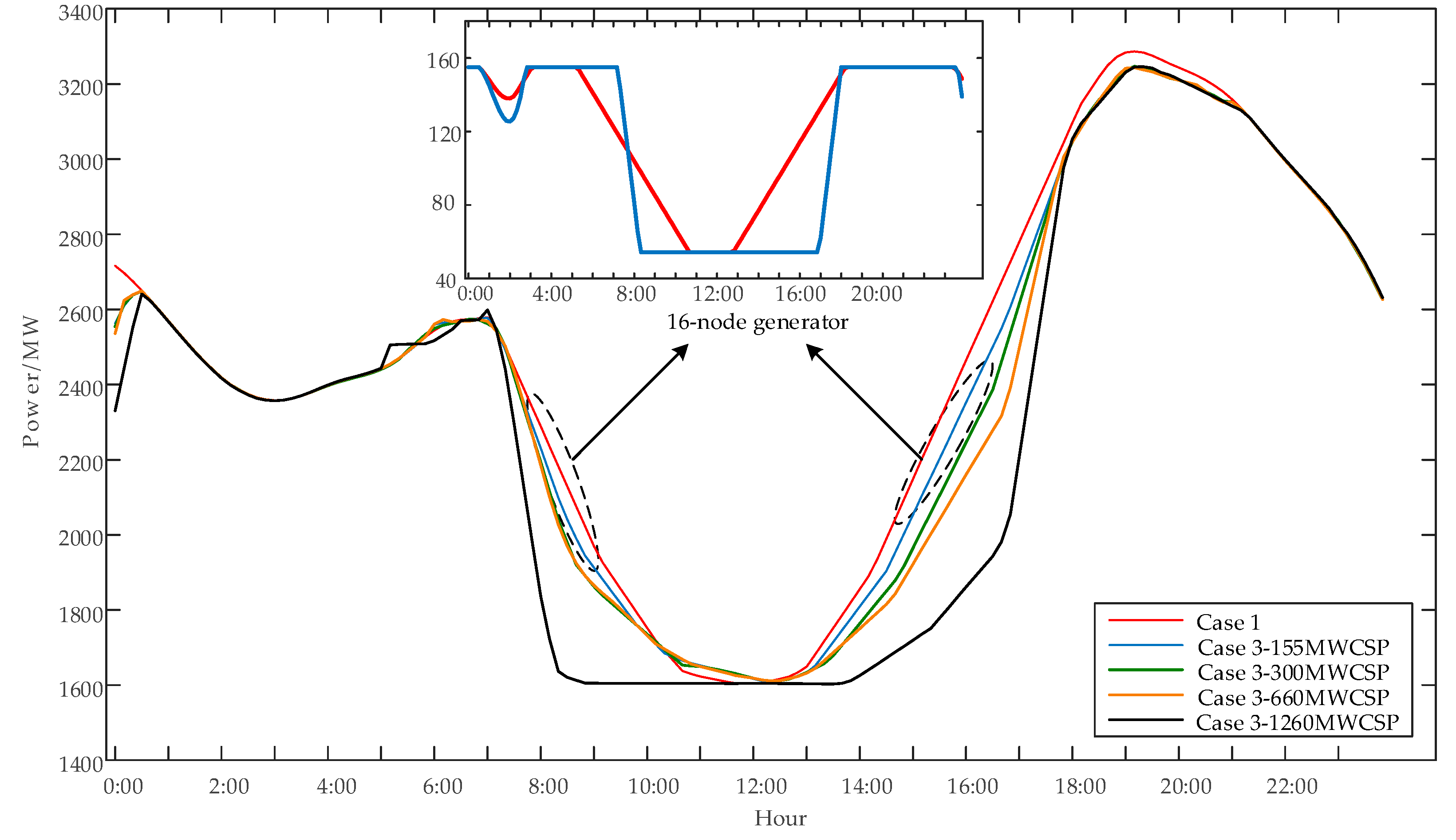
(1) The simplified static energy flow model for CSP station is enough to embody the dispatch-ability of TSS. With regard to the power system operation, the CSP station can operate in the TSS mode, for storing the solar thermal energy during the midday (9:00–14:00) and generating electricity during the sunset (16:00–21:00) to supply the power shortage of duck curve using its faster ramp rate.

(2) The mitigation strategy adopting the proposed optimization model can increase the maximum PV penetration up to 25.62% and reduce the maximum lost load down to 0.0663MW in the IEEE-24 node system. It ensures the economical operation of the system and the reliability of power supply. Hence, the duck curve becomes fatter for accommodating more PV due to the operational flexibility of CSP station.

The above indicates that the CSP station will play a significant supporting role in the future high penetration of renewable energy power system, with the breakthrough of CSP technology and the increase of its installed capacity.

References

1. Malinowski, M.; Leon, J.I.; Abu-Rub, H. Solar photovoltaic and thermal energy systems: Current technology and future trends. Proc. IEEE 2017, 105, 2132–2146. [Google Scholar] [CrossRef]
2. International Renewable Energy Agency. 2018. Available online: http://www.irena.org (accessed on 23 April 2019).
3. Bocca, A.; Bergamasco, L.; Fasano, M.; Bottaccioli, L.; Chiavazzo, E.; Macii, A.; Asinari, P. Multiple-regression method for fast estimation of solar irradiation and photovoltaic energy potentials over Europe and Africa. Energies 2018, 11, 3477. [Google Scholar] [CrossRef]
4. Li, X.; Yao, L.; Hui, D. Optimal control and management of a large-scale battery energy storage system to mitigate fluctuation and intermittence of renewable generations. J. Mod. Power Syst. Clean Energy 2016, 4, 593–603. [Google Scholar] [CrossRef] [Green Version]
5. Sioshansi, F.P. California’s ‘Duck Curve’ Arrives Well Ahead of Schedule. Electr. J. 2016, 29, 71–72. [Google Scholar]
6. Wirfs-Brock, J. IE Questions: Why is California Trying to Behead the Duck? Inside Energy: Denver, CO, USA, 2014. [Google Scholar]
7. Hernandez, J.C.; Medina, A.; Jurado, F. Optimal allocation and sizing for profitability and voltage enhancement of PV systems on feeders. Renew. Energy 2007, 32, 1768–1789. [Google Scholar] [CrossRef]
8. Ning, J.; Tang, Y.; Chen, Q.; Wang, J.; Zhou, J.; Gao, B. A bi-level coordinated optimization strategy for smart appliances considering online demand response potential. Energies 2017, 10, 525. [Google Scholar] [CrossRef]
9. Sanchez-Sutil, F.; Cano-Ortega, A.; Hernandez, J.C.; Rus-Casas, C. Development and calibration of an open source, low-cost power smart meter prototype for PV household-prosumers. Electronics 2019, 8, 878. [Google Scholar] [CrossRef]
10. Parizy, E.S.; Bahrami, H.R.; Choi, S. A low complexity and secure demand response technique for peak load reduction. IEEE Trans. Smart Grid 2019, 10, 3259–3268. [Google Scholar] [CrossRef]
11. Zhou, N.; Liu, N.; Zhang, J.; Lei, J. Multi-objective optimal sizing for battery storage of PV-based microgrid with demand response. Energies 2016, 9, 591. [Google Scholar] [CrossRef]
12. Wang, W.; Liu, J.; Zeng, D.; Niu, Y.; Cui, C. Modeling for condensate throttling and its application on the flexible load control of power plants. Appl. Therm. Eng. 2016, 95, 303–310. [Google Scholar] [CrossRef]
13. Denholm, P.; O’Connell, M.; Brinkman, G.; Jorgenson, J. Overgeneration from Solar Energy in California: A Field Guide to the Duck Chart; NREL/TP-6A20–65023; National Renewable Energy Laboratory: Golden, CO, USA, 2015. [Google Scholar]
14. Doroshenko, M.; Keshav, S.; Rosenberg, C. Flattening the duck curve using grid-friendly solar panel orientation. Proc. ACM Energy 2018, 2018, 375–377. [Google Scholar]
15. Pan, K.; Guan, Y.; Watson, J.; Wang, J. Strengthened MILP formulation for certain gas turbine unit commitment problems. IEEE Trans. Power Syst. 2016, 31, 1440–1448. [Google Scholar] [CrossRef]
16. Howlader, H.O.R.; Sediqi, M.M.; Ibrahimi, A.M.; Senjyu, T. Optimal thermal unit commitment for solving duck curve problem by introducing CSP, PSH and demand response. IEEE Access 2018, 6, 4834–4844. [Google Scholar] [CrossRef]
17. Torabi, R.; Alvaro, G.; Morgado-Dias, F. The duck curve characteristic and storage requirements for greening the island of Porto Santo. In Proceedings of the International Conference on Energy and Sustainability in Small Developing Economies, Funchal, Portugal, 9–12 July 2018. [Google Scholar]
18. Zhao, H.; Wu, Q.; Hu, S.; Xu, H.; Rasmussen, C.N. Review of energy storage system for wind power integration support. Appl. Energy 2015, 137, 545–553. [Google Scholar] [CrossRef]
19. Du, E.; Zhang, N.; Hodge, B.M.; Wang, Q.; Lu, Z.; Kang, C.; Kroposki, B.; Xia, Q. Operation of a high renewable penetrated power system with CSP plants: A look-ahead stochastic unit commitment model. IEEE Trans. Power Syst. 2019, 34, 140–151. [Google Scholar] [CrossRef]
20. Gao, Y.; Xue, F.; Yang, W.; Yang, Q.; Sun, Y.; Sun, Y.; Liang, H.; Li, P. Optimal operation modes of photovoltaic-battery energy storage system based power plants considering typical scenarios. Prot. Control Mod. Power Syst. 2017, 2, 36. [Google Scholar] [CrossRef]
21. Wang, Y.; Lou, S.; Wu, Y.; Wang, S. Co-allocation of solar field and thermal energy storage for CSP plants in wind-integrated power system. IET Renew. Power Gener. 2018, 12, 1668–1674. [Google Scholar] [CrossRef]
22. Du, E.; Zhang, N.; Hodge, B.M.; Wang, Q.; Kang, C.; Kroposki, B.; Xia, Q. The role of concentrating solar power toward high renewable energy penetrated power systems. IEEE Trans. Power Syst. 2018, 33, 6630–6641. [Google Scholar] [CrossRef]
23. Santos-Alamillos, F.J.; Pozo-Vázquez, D.; Ruiz-Arias, J.A.; Von Bremen, L.; Tovar-Pescador, J. Combining wind farms with concentrating solar plants to provide stable renewable power. Renew. Energy 2015, 76, 539–550. [Google Scholar] [CrossRef]
24. Qi, F.; Wen, F.; Liu, X.; Salam, M.A. A residential energy hub model with a concentrating solar power plant and electric vehicles. Energies 2017, 10, 1159. [Google Scholar] [CrossRef]
25. Luo, Q.; Ariyur, K.B.; Mathur, A.K. Control-oriented concentrated solar power plant model. IEEE Trans. Control Syst. Technol. 2016, 24, 623–635. [Google Scholar] [CrossRef]
26. Dominguez, R.; Conejo, A.J.; Carrion, M. Operation of a fully renewable electric energy system with CSP plants. Appl. Energy 2014, 119, 417–430. [Google Scholar] [CrossRef]
27. Fang, L.; Dong, H.; Ding, K.; Wang, N. Peak shaving strategy of power grid with concentrating solar power. In Proceedings of the 2017 13th IEEE Conference on Automation Science and Engineering (CASE), Xi’an, China, 20–23 August 2017; pp. 1633–1638. [Google Scholar]
28. Du, E.; Zhang, N.; Kang, C.; Miao, M.; Tian, X. Exploring the flexibility of CSP for wind power integration using interval optimization. In Proceedings of the 2016 IEEE Power and Energy Society General Meeting, Boston, MA, USA, 17–21 July 2016. [Google Scholar]
29. Correa-Posada, C.M.; Morales-España, G.; Dueñas, P.; Sánchez-Martín, P. Dynamic ramping model including intraperiod ramp-rate changes in unit commitment. IEEE Trans. Sustain. Energy 2017, 8, 43–50. [Google Scholar] [CrossRef]
30. California ISO. What the Duck Curve Tells Us about Managing a Green Grid; California ISO: Folsom, CA, USA, 2015. [Google Scholar]
31. Cheng, D.; Mather, B.A.; Seguin, R.; Hambrick, J.; Broadwater, R.P. Photovoltaic (PV) impact assessment for very high penetration levels. IEEE J. Photovolt. 2016, 6, 295–300. [Google Scholar] [CrossRef]
Figure 1. Structure of the concentrating solar power (CSP) station.
Energies 12 03521 g001
Figure 2. The simplified operation model of CSP station.
Energies 12 03521 g002
Figure 3. The flowchart of developing CSP model.
Energies 12 03521 g003
Figure 4. The regulation capability of the unit.
Energies 12 03521 g004
Figure 5. The CAISO predicted duck curve [30].
Energies 12 03521 g005
Figure 6. Diagram of mitigation strategy using the CSP station.
Energies 12 03521 g006
Figure 7. The schematic diagram of optimization model.
Energies 12 03521 g007
Figure 8. The modified IEEE-24 node simulation system.
Energies 12 03521 g008
Figure 9. The predicted power of photovoltaic (PV) power station and total load on three typical days. (a) The spring equinox; (b) The summer solstice; (c) The winter solstice.
Energies 12 03521 g009
Figure 10. Comparative results of case 1, case 2, and case 3.
Energies 12 03521 g010
Figure 11. The output power curve of all generators in case 1 and case 3 at different PV penetration.
Energies 12 03521 g011
Figure 12. The net load power curve when PV penetration is 12.25%.
Energies 12 03521 g012
Figure 13. The net load curve with different CSP station replacement capacity.
Energies 12 03521 g013