Investigation of Hydraulic Fracturing Behavior in Heterogeneous Laminated Rock Using a Micromechanics-Based Numerical Approach

Abstract

Understanding hydraulic fracturing mechanisms in heterogeneous laminated rocks is important for designing and optimizing well production, as well as for predicting shale gas production. In this study, a micromechanics-based numerical approach was used to understand the physical processes and underlying mechanisms of fracking for different strata orientations, in-situ stresses, rock strengths, and injection parameters. The numerical experiments revealed a very strong influence of the pre-existing weakness planes on fracking. Geological models for rock without weakness planes and laminated rock behave very differently. Most simulated fractures in the rock without weakness planes were caused by tensile failure of the rock matrix. In an intact rock model, although a radial damage zone was generated around the injection hole, most of the small cracks were isolated, resulting in poor connectivity of the fracture network. For rock models with pre-existing weakness planes, tension and shear failure of these structural planes formed an oval-shaped network. The network was symmetrically developed around the injection well because the strength of the pre-existing weakness planes is generally lower than the rock matrix. The research shows that the angular relations between the orientation of the structural planes and the maximum horizontal stress, as well as the in-situ stress ratios, have significant effects on the morphology and extent of the networks. The strength of the pre-existing weakness planes, their spacing, and the injection rate can dramatically influence the effectiveness of hydraulic fracturing treatments.

1. Introduction

Hydraulic fracturing is an important technology for shale gas developement [1]. This technology depends on multiple parameters, and fracture formation is dominated by several factors, e.g., the in-situ stress, the rock mass properties, and the injection rates [1,2]. The seepage pathway of fluid flow in a fractured rock mass is mainly controlled by the geometry, pattern, and heterogeneity of the hydraulic fracture network [3,4,5,6]. Therefore, the quality of the artificially modified fracture network is a critical factor in practical applications [7,8].

The anisotropic mechanical properties of rocks play an important role in the damage and stability of rock structures. Zhang et al. [9] revealed that the deformation of Callovo-Oxfordian claystone depends on the orientation of the major principal stress to the bedding and the claystone strength depends on the loading path and direction with respect to the bedding. Valente et al. [10] analyzed the mechanisms of parallel-to-bedding cracking through a sensitivity analysis and using a numerical Non-Linear Elastic Fracture Mechanics model. Kakouris et al. [11] proposed a phase-field formulation within a material point method to simulate brittle fracture in anisotropic media. Bleyer et al. [12] used a phase-field approach to model anisotropic fracture phenomena of elastic brittle materials. Shales are anisotropic due to their laminated structure [13]. The geometry and pattern of a hydraulic fracture network are complex and often poorly understood in the field, despite the use of micro-seismic interpretation [14,15,16].

Although the formation of fractures around injection wells has been extensively studied using computational, experimental, and field methods, the influence of pre-existing fractures on hydraulic fracturing still needs further study [17]. During fracking, natural structural planes can influence the propagation of hydraulic fractures [17,18,19]. In the last few years, reduced-scale experiments and simulations have been extensively carried out to elucidate the mechanisms and process of the interaction between induced and natural fractures. The existing natural fractures not only influence the propagation of hydraulic fractures, but can also be activated by the high-pressure injection fluid [20]. Therefore, the interaction between the induced and natural fractures must be considered before hydraulic fracturing takes place. Various analyses have been reported in the literature to study the interaction between hydraulic and natural fractures in shale reservoirs [8]. However, mechanisms for the formation of hydraulic fracture networks and how the failure modes are affected by weak structural planes is still poorly understood [7,13].

Among the various models, the linear elastic and isotropic constitutive model, together with the linear failure criterion, are the most frequently used methods [21,22,23]. However, shale has anisotropic properties for deformation and strength because of its laminated rock mass structure [5]. A few analytical solutions for fracture initiation and propagation in anisotropic formations have been developed to evaluate the fracturing [8]. However, the coupling between the anisotropic damage and permeability variation in shale formations is a dynamic process, and the evolution of hydraulic fracturing is difficult to model and simulate.

Numerical modeling provides an approach to understand the hydraulic fracture initiation and propagation processes. Numerous modeling efforts have been conducted to understand the process and mechanism of hydraulic fracturing [24,25,26,27,28]. Miehe et al. [29] studied the hydraulic fracturing of a fluid-saturated porous media using a phase-field modeling method. Wilson et al. [30] proposed a theoretical method implementing a phase-field approach to study the mechanisms of hydraulic fracturing. Ehlers et al. [31] studied hydraulic fracturing processes based on the theory of porous media and a phase-field fracture model. Despite this arsenal of insights, techniques, and specialized knowledge, there is still a lack of understanding of the dynamic fracture propagation and the failure mechanisms in shale formations. Additionally, there are still a lack of satisfactory models that can explicitly represent the heterogeneity characteristics of shale formations and simulate the coupling between stress, fluid flow, and damage in ways that can be easily visualized [4].

In shale fracturing simulation, the heterogeneity of reservoirs is one of the challenges that influence the fracturing and productivity prediction. Previous studies have indicated that a small change in the properties could result in a significant difference in the propagation direction and pattern of hydraulic fractures [32,33,34]. In addition, another obstacle lies in understanding the irregular flow paths in heterogeneous formations [35,36,37].

To study coupled flow-damage problems, a coupled flow-stress-damage (FSD) model was put forward by Tang et al. [38,39,40,41,42] to simulate the fracture process under boundary stress and hydraulic conditions. This model was improved to incorporate heterogeneity in micro-mechanical properties [33]. The most outstanding characteristic of the FSD model is that new fractures can be produced during the loading process. Discontinuous mechanical problems can be handled by integrating a strength reduction method into the model. In addition, the initiation and propagation of natural fractures are dynamic in the model. The interactions between the pre-existing and induced hydraulic fractures are automatically calculated. The FSD coupling approach was selected for the research presented in this paper because of its advantages and ability to simulate the interactions between induced hydraulic fractures and pre-existing fractures in heterogeneous rock.

In this study, the evolution of the hydraulic fracturing process is simulated in a model of anisotropic shale at the laboratory scale in which the shale microstructure was explicitly represented by inserting one or two sets of parallel discontinuities into the model. Through a series of modeling experiments, the influence of the discontinuities on the hydraulic fracturing was extensively investigated. In addition, hydrofracturing simulations were conducted to assess the influences of the in-situ stress ratio, the mechanical properties of the discontinuities, the discontinuity spacing, and the injection rate on the evolution of hydraulic fractures.

2. Modeling Methodology

The FSD coupled approach was derived from damage mechanics and statistical theory by considering the deformation of an elastic material containing a random initial distribution of micro-factures [35,38,39,40,41,42]. This modeling approach can simulate nonlinear rock behaviors and macroscopic rock fractures without knowledge of where and how the fractures will occur. Compared with other numerical methods, there are two distinct features: (1) By introducing the heterogeneity of rock parameters, nonlinear behavior in rock can be simulated, and (2) by introducing elastic modulus reduction after element failure, discontinuum mechanics can be simulated in a continuum mechanics model. For a more detailed description of the method, readers are referred to the references.

To simulate the progressive failure of the heterogeneous, permeable rock mass, the FSD coupled model assumes [38,39,40,41,42] that (1) the flow of fluid in the model follows the Biot consolidation theory; (2) the model material is assumed to be elastic-brittle with residual strength and its failure can be described by elastic damage theory; (3) the Mohr–Coulomb criterion and the maximum tensile strength criterion can be used to define the tensile failure and shear failure of the rock; and (4) the permeability coefficient of the rock material is varied with the stress in an elastic state and increases dramatically according to a deformation-dependent law when the element progresses towards the failure stage. The continuum damage principle is applied and the fracture is presented as the damage zone. The basic equations used in the analysis are as follows:

Equilibrium equation:

$${\partial }^2{\sigma }_{ij}/\partial x_{ij}{}^2+\rho X_j=0 (i,j=1,2,3)$$

(1)

Strain-displacement equation:

$${\epsilon }_{ij}=\frac{1}{2}(u_{i,j}+u_{j,i})$$

(2)

Constitutive equation:

$${\sigma }_{ij}^{\prime }={\sigma }_{ij}-\alpha p{\delta }_{ij}=\lambda {\delta }_{ij}{\epsilon }_v+2G{\epsilon }_{ij}$$

(3)

$$△n=p/Q-\alpha {\epsilon }_v=p/H-{\sigma }_{ii}/3H$$

(4)

Seepage equation:

$$k{\nabla }^{2}p=1/Q\cdot \partial p/\partial t-\alpha \cdot \partial {\epsilon }_v/\partial t$$

(5)

where ${\sigma }_{ij}$ is the total stress in the ij-plane, ${\sigma }_{ij}^{\prime }$ is the effective stress in the ij-plane, $\rho$ is the density, $X_j$ is the body force in the j-th direction, $u$ is the element displacement, ${\epsilon }_{ij}$ is the strain in the ij-plane, ${\epsilon }_v$ is the volumetric strain, $p$ is the pore water pressure, $\lambda$ is the Lame coefficient, ${\delta }_{ij}$ is the Kronecker constant, $G$ is the shear modulus, $k$ is the coefficient of permeability, $\alpha$ is the pore-fluid pressure coefficient (dimensionless), $H$ and $R(Q,\alpha )$ represent the Biot’s constant, $\beta$ is a coupling parameter that reflects the influence of stress on the permeability coefficient, $\xi$ is a damage factor of permeability (dimensionless), $1/R$ represents the water capacity change due to changes in water pressure, $1/H$ represents the change in the overall volume of the media due to changes in water pressure, and $1/Q$ represents the amount of water squeezed into the porous media under the action of water pressure without changing the volume of the porous media.

The relationship between the $Q$, $R$, $H$, and $\alpha$ is

$$\alpha =(3\lambda +2G)/3H=2(1-\mu )G/3(1-2\mu )H=E/3(1-2\mu )H=K^{\prime }/H$$

(6)

$$1/R=1/Q+\alpha /H$$

(7)

where $E$ is the elastic modulus, $K^{\prime }$ is the bulk modulus, and $\mu$ is the Poisson’s ratio. In the process of steady flow, the flow tends to be stable as the pore water dissipates. Therefore, the value of Q is very large; assuming $Q=\infty$, Equation (7) can be simplified as

$$1/R=\alpha /H$$

(8)

A pore volume change of $\Delta n$ causes a flow rate change. The permeability coefficient $k$ is a function of the pore volume change $\Delta n$. Therefore, the coupling equation can be described as

$$k(\sigma ,p)=\xi k_0{e}^{\beta △n}=\xi k_0{e}^{\beta (p/R-{\sigma }_{ii}/3H)}=\xi k_0{e}^{-\beta ({\sigma }_{ii}/3-\alpha p)}$$

(9)

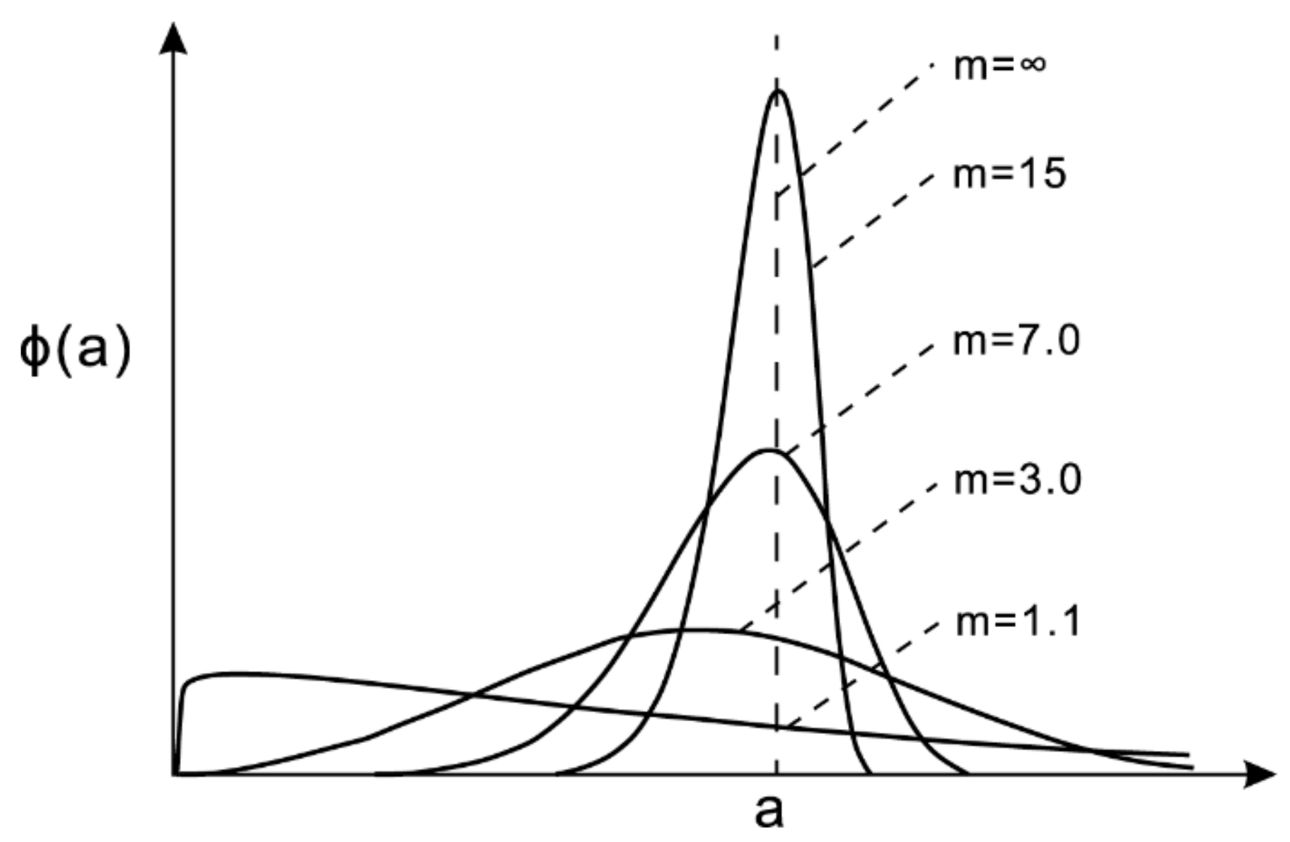
Equation (9) is a negative exponential function that is applied to describe the relationship between stress and damage. The most important hypothesis reflected in the FSD model is that a heterogeneous distribution of rock strength causes rock failure behavior. The rock medium is assumed to be locally heterogeneous by randomly assigning the Young’s modulus and compressive strength to each element in a Weibull distribution [39]:

$$f(s)=\frac{m}{s_0}{(\frac{s}{s_0})}^{m-1}\exp {(-\frac{s}{s_0})}^m$$

(10)

where $s$ is the mechanical parameter of the elements, such as elastic modulus or strength. The scale parameter $s_0$ is related to the average value of the element parameter, and the parameter $m$ defines the homogeneity index; a higher value of $m$ represents a more homogeneous material. The strength distribution with different m values is illustrated in Figure 1.

In the FSD coupled model, the coupled effects of flow, stress, and damage on the fractures and the permeability of rock mass are considered [44]. Both the tensile and shear failure modes are considered in the model calculation. The maximum tensile strain criterion and the Mohr–Coulomb criterion are used to define the types of deformation and breakdown. According to the elastic damage mechanics, the elastic modulus of the damaged material can be defined as [39]

$$E=(1-D)E_0$$

(11)

where D represents the damage variable, and E and $E_0$ are the elastic modulus of the damaged and the undamaged elements, respectively.

When the tensile stress reaches its tensile strength,

$${\sigma }_3\le -f_i$$

(12)

where $f_i$ is the tensile strength of the rock element. Then, the damage variable can be described as [39]

$$D=\left\{\begin{array}{l}0,\hspace{1em}\overline{\epsilon }\le {\epsilon }_{\mathrm{to}}\\ 1-\frac{f_{tr}}{E_0\epsilon },\hspace{1em}\\ 1,\hspace{1em}\overline{\epsilon }\le {\epsilon }_{tu}\end{array}\right.{\epsilon }_{to}\le \overline{\epsilon }<{\epsilon }_{tu}$$

(13)

where $f_{tr}$ is the residual tensile strength of the element, $\overline{\epsilon }$ is the equivalent principal strain, ${\epsilon }_{to}$ is the threshold strain, and ${\epsilon }_{t\mathrm{u}}$ is the maximum tensile strain of the element. Then, the permeability can be described as

$$\begin{gathered} k(\sigma ,p)=\xi k_0{e}^{\beta △n}=\xi k_0{e}^{\beta (\frac{p}{R}-\frac{1}{3H}{\sigma }_{ii})}=\xi k_0{e}^{-\beta (\frac{{\sigma }_{ii}}{3}-\alpha p)} \\ k=\left\{\begin{array}{ll}{k}_0{e}^{-\beta ({\sigma }_{ii}-\alpha p)}& D=0\\ \xi k_0{e}^{-\beta ({\sigma }_{ii}-\alpha p)}& 0<D<1\\ {\xi }^{\prime }{k}_0{e}^{-\beta ({\sigma }_{ii}-\alpha p)}& D=1\end{array}\right. \end{gathered}$$

(14)

where $\xi$ is a damage factor of permeability, $k_0$ is the initial coefficient, $\alpha$ is the pore-fluid pressure coefficient (dimensionless), $\beta$ is a coupling parameter, and $p$ is the pore water pressure.

In the FSD coupled model, tensile failure of the element occurs if the element’s strength is smaller than the minor principal stress, and shear failure occurs when the compressive or shear stress satisfies the Mohr–Coulomb failure criterion:

$$F={\sigma }_1^{\prime }-{\sigma }_3^{\prime }\frac{1+\sin {\varphi }^{\prime }}{1-\sin {\varphi }^{\prime }}\ge f_c^{\prime }$$

(15)

where ${\sigma }_1^{\prime }$ and ${\sigma }_3^{\prime }$ are the maximum and minimum principal effective stresses, ${\varphi }^{\prime }$ is the effective angle of friction, and $f_c^{\prime }$ is the compressive failure strength. In this case, the damage factor under uniaxial compression can be described as

$$D=\left\{\begin{array}{ll}0& \overline{\epsilon }<{\epsilon }_{c\mathrm{u}}\\ 1-\frac{f_{cr}}{E_0\epsilon }& \epsilon \ge {\epsilon }_{\mathrm{co}}\end{array}\right.$$

(16)

where $f_{cr}$ is the residual compressive strength and ${\epsilon }_{c\mathrm{u}}$ is the maximum compressive strain. In this case, the permeability can be defined by

$$k=\left\{\begin{array}{ll}{k}_0{e}^{-\beta ({\sigma }_{ii}-\alpha p)}& D=0\\ \xi e^{-\beta ({\sigma }_{ii}-\alpha p)}& D>0\end{array}\right.$$

(17)

3. Model Setup for Hydraulic Fracturing Simulation

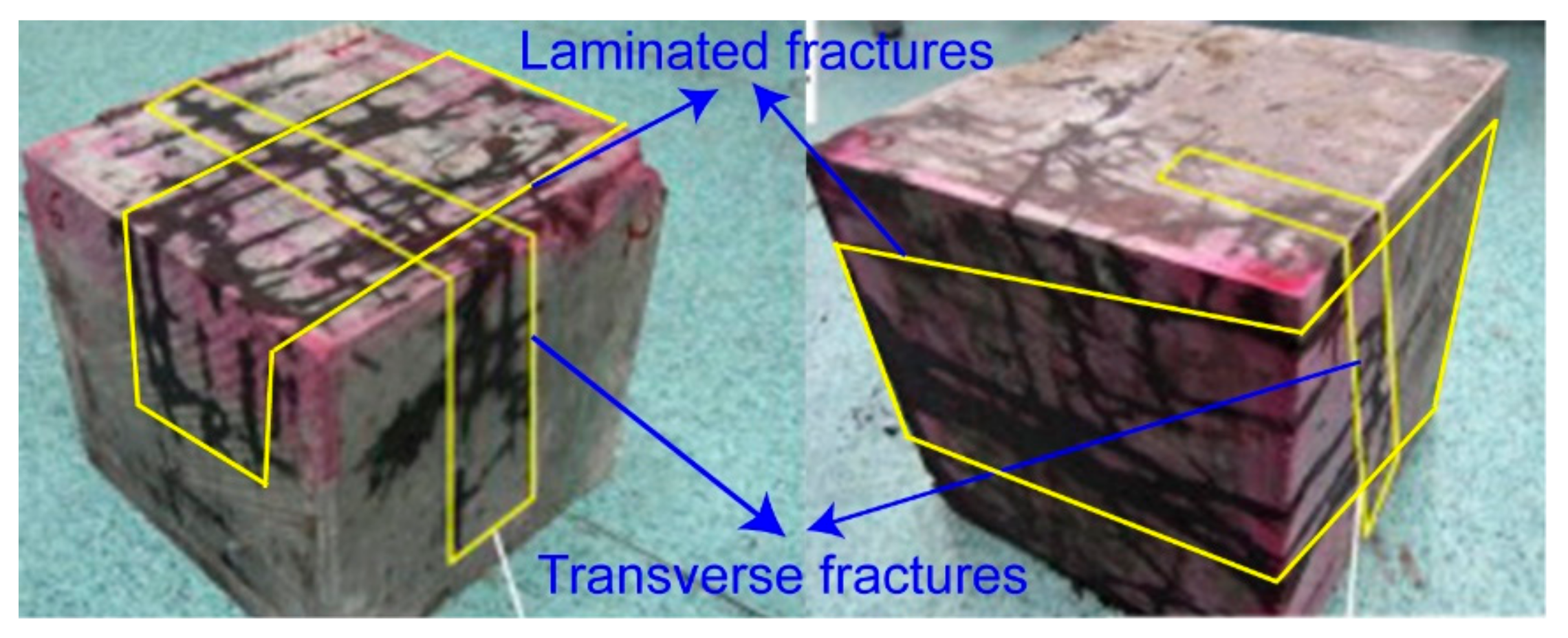
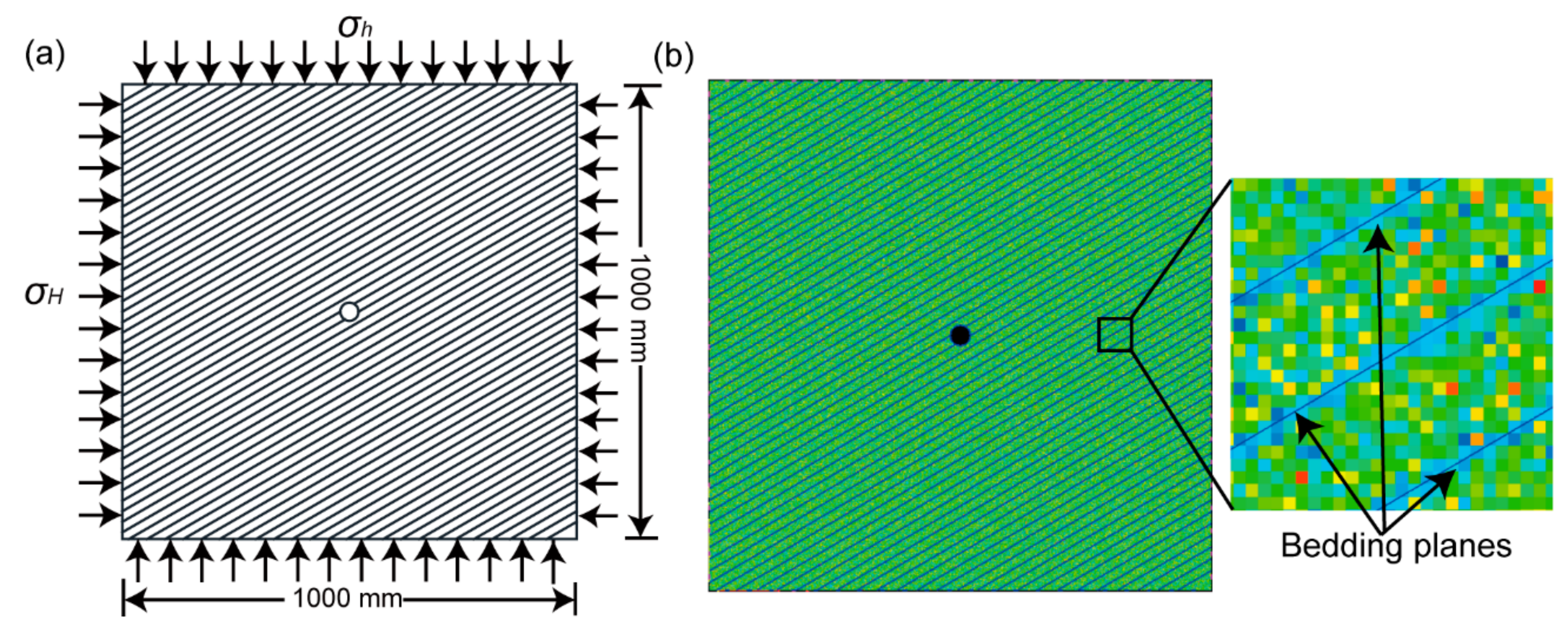
For this study, bedding joints and crossing joints were the structure planes considered in the modeling simulation. Figure 2 shows the basic geometry and model setup, which represents a 2D horizontal section of a reservoir. The model is composed of 250,000 (500 × 500) identical 2 mm square elements. The element size is small enough for the accuracy requirement of the model, and no further re-meshing was needed. A vertical wellbore with a radius of 20 mm is in the center of the model and serves as the injection hole during the simulation.

In models with structural planes, the bedding angles are 0°, 15°, 30°, 45°, 60°, and 75°. The spacings of structural planes are 1.0, 2.0, and 3.0 times the radius of the injection hole. As shown in Figure 2, a constant stress boundary condition was used to simulate an analogous in-situ stress environment. For the base model, the stresses in the x (σ_H) and y (σ_h) directions on the model boundary were 12 MPa and 8 MPa, respectively. In the cross joint models, two sets of structural planes with inclination angles of 45° and 135° were used. The stresses on the model boundary were set to 12 MPa and 8 MPa or 10 MPa and 10 MPa, respectively. The hydraulic fracturing process was simulated under the condition of a constant injection rate of 0.15 m³·s⁻¹·m⁻¹.

The material mechanical parameters used in the FSD coupled model were calibrated through a series of trial-and-error experiments [44]. The microparameters were calibrated to match the macro properties of the Longmaxi shale rock, including the elastic modulus, peak strength, and Poisson’s ratio. The mesoscopic physical and mechanical parameters of the model used in this study are shown in

Table 1. Mean material mechanical properties for the numerical models.

Index	Structural Plane	Rock Matrix
Homogeneity index, m	3	3
Elastic modulus, E0 (GPa)	15	50
Poisson’s ratio, ν	0.3	0.2
Internal friction angle, φ (°)	25	40
Compressive strength, σc (MPa)	150	300
Tensile strength, σt (MPa)	15	30
Permeability coefficient, k0 (m·d−1)	0.003	0.001
Porosity (%)	0.3	0.1
Coupling coefficient, β	0.01	0.01
Coefficient of pore-water pressure, a	0.8	0.5

.

4. Results of Numerical Modeling

4.1. Fracture Distribution for the Base Model

The failure process and hydraulic fracture characteristics in heterogeneous rocks without the influence of bedding joints (base model) were studied first; the results serve as a base-case for comparison with other results presented in this paper. Figure 3 shows the progressive fracturing process of the model (in-situ stress ratio σ_H/σ_h = 1.5, injection rate = 0.15 m³·d⁻¹·m⁻¹). This model is the base model for the following comparative study.

As illustrated in Figure 3, the fracturing can be divided into five stages, depending on the fracture formation process:

(1) Stress accumulation. A few micro-units clustered around the injection hole with a lower strength and stiffness are damaged (Figure 3b). Since the tensile strength is far less than the compressive strength, and there is no preferential location around the injection hole for fractures to initiate, the location and orientation of the fracture initiation are unpredictable;

(2) Small fracture formation. The continuous injection increases the pore pressure around the injection hole, and many small fractures occur in all directions around the injection hole (Figure 3c). Although a radial damage zone was generated, most of the small fractures were isolated with poor connectivity;

(3) Hydraulic fracture initiation. With further injection, an embryonic network of connected hydraulic fractures gradually forms around the injection hole due to propagation and coalescence of the fractures (Figure 3d);

(4) Hydraulic fracture propagation. The dominant hydraulic fractures grow and extend parallel to the direction of σ_H (Figure 3e). Meanwhile, many small hydraulic fractures occur around the main fractures as the injection continues;

(5) Decay in fracture propagation. The rate of fracture propagation and the growth in the area with new fractures gradually decline because the constant injection rate cannot sustain the fracture growth far away from the injection hole. A large and growing proportion of the injection fluid is scattered into the fractures and the rock strata. The characteristics of fluid leak-off are related to fracture connectivity and the injection rate. In this example, both the size of the simulated area and the number of fractures achieved a peak and an oval-shaped fracture network eventually developed (Figure 3f).

4.2. Morphology of Fracture Networks in Laminated Rocks

The presence of structural weakness planes such as bedding in reservoir rock affects the response and effectiveness of hydraulic fracturing [7,8]. The pre-existing structural planes, such as bedding planes and tectonic joint sets, influence the volume and shape of the fractured zone in laminated shale formations [3,17]. In general, the strength of natural structural planes is lower than the strength of the rock matrix, and these structures are particularly vulnerable to damage and failure during hydraulic fracturing [17].

Figure 4 shows the modeled fracture networks under the influence of different pre-existing structural planes (bedding joints). In contrast with the base case model, the most remarkable feature is that the orientation of the structural planes exerts an important influence on the propagation direction of the hydraulic fractures. Under a constant injection rate, the structural planes were activated and damaged to form the framework of the hydraulic fracture network. In these models, the pore water pressure propagated throughout a large area of the model through these fractures.

The results are in good agreement with most of the laboratory experiments and numerical results. For instance, Guo. et al. [7] studied the propagating rules of fractures in shale through a true triaxial test system and found that the hydraulic fractures easily propagate along with the natural fractures (Figure 5). Liu et al. [45] studied the influence of natural fractures on the propagation geometry of hydraulic fractures through a tri-axial fracturing system and found that the horizontal differential stress and the angle between the maximum horizontal principal in situ stress and the pre-fracture are the dominating factors for the initiation and propagation of hydraulic fractures. He et al. [46] studied the hydraulic fracturing through the displacement discontinuities method and found that the pre-existing fractures were favorable to the formation of the hydraulic fracture network. Zhou et al. [47] studied the near-borehole fracture propagation in a laminated reservoir rock using PFC2D and found that the hydraulic fracture propagation in a laminated reservoir is controlled by both in situ stress and the bedding surface.

Apart from the above common features, there are some intriguing differences between the models with different structural plane orientations. For models with low angles (0°–15°), the structural planes control the initiation and propagation of the hydraulic fracture networks. However, as the angle increases, more small-scale transverse fractures occur in conjunction with the main fracture networks. When the orientations of the structural planes are approximately parallel to the direction of σ_H (0° to 15°, Figure 4a,b), the initiation and propagation of hydraulic fractures tend to develop along the structural planes and form straight fractures. When the angle increases slightly (30° to 45°, Figure 4c,d), hydraulic fractures still occur along the structural planes, but many secondary fractures also occur. These secondary fractures are aligned in the direction of σ_H and are interconnected with the main hydraulic fractures. The increase in the pore water pressure causes a high tensile stress area at the fracture tips along the structural planes. As the tensile strength is exceeded, the fractures can grow in a direction parallel to σ_H.

For models with steeply inclined structural planes (60°–75°, Figure 4e,f), some obvious changes occur in the morphology of the fracture networks. The maximum horizontal stress plays an increasingly important role in the initiation and propagation of the hydraulic fractures. As the angle increases, more hydraulic fractures occur through the rock between the structural planes in conjunction with the fracturing along the structural planes. Furthermore, the roughness of hydraulic fractures increased significantly with the increased angle of the structural planes. In this case, both the structural planes and the maximum horizontal stress determine the evolution of the simulated hydraulic fractures.

4.3. Evolution of Hydraulic Fractures in Laminated Rocks

Hydraulic injection and fracturing is a dynamic failure process that involves a complicated hydro-mechanical coupled interaction [1]. When high-pressure fracture fluids are injected into a target formation, a sharp increase in pore pressure and adjustment of the stress field will be induced in the affected area [22]. In this case, pre-existing open fractures and new fractures are the two main ways to develop a fracture network for the desorption and migration of shale gas. The dramatic changes in pore water pressure resulting from the fluid injection can generate significant changes in the effective stresses [20]. In addition, the total stress changes induced by the high-pressure fluid are influenced by the geometry of the fractures in the reservoir and the variations in the physical-mechanical properties of the fractured reservoir and surrounding strata [44]. The critical pressure necessary for the initiation of a new hydraulic fracture or fracturing along a natural weakness plane depends on the stress state in the rock and the structural planes. In shale, tensile failure plays an important role because the tensile strength of the structural planes can be very low. In laboratory experiments, tensile failure of the rock matrix usually shows up as the initiation of a fracture and the accumulation and coalescence of many small tensile failures, leading to macroscopic shear failure of the rock mass. This is why combined tension-shear failure was considered as a widespread phenomenon during hydraulic fracturing. When the elevated pore pressure exceeds the sum of the tensile strength of the rock and the minimum principal stress, tensile failure can occur and propagate.

Figure 6 shows the minimum principal stress field caused by the initiation and propagation of hydraulic fractures in the model with different structural plane orientations. As expected, when small fractures occur, they are associated with tensile stresses in the adjacent elements near the fracture tip [23]. The tensile stress and the heterogeneity in the mechanical properties initiate the fractures and drive the propagation of these fractures, resulting in the coalescence of small fractures.

It is generally known that acoustic emission occurs due to strain energy release caused by rock failure and slip along rock mass discontinuities. Acoustic emission events can be induced by fracture initiation and propagation and by failure along natural bedding planes [20]. The model can track the location and type of acoustic emission events. The element failures tend to occur in the laminated layers around the injection hole due to their lower strength and Young’s modulus. Detailed information on how acoustic emission events are modeled can be found in reference [38].

Figure 7 shows a case where acoustic emissions occur during the simulation of hydraulic fracturing. Although a fracture network dominated by shear failure is expected to create the most efficient seepage pathways for shale gas recovery [43,48,49], the simulation results show that nearly all the failed elements experienced tensile failure and the hydraulic fracturing of rock is essentially a tensile failure phenomenon at the micro-level. In practice, tensile fractures close easier than shear fractures after fluid injection. This is the primary reason that the fracture fluids contain propping agents, such as sand or aluminum oxide pellets, which are suspended in the fracture fluids and used to hold the fractures open after the pumping stops.

In the early stages of fracturing, nearly all the small fractures are initiated at the weak structural planes. The locations of weak structural planes and reservoir heterogeneity determined the initiation points for the small fractures. The subsequent growth and propagation of fractures are affected by the angular relation between the orientations of the structural planes and σ_H. The hydraulic fractures tend to grow parallel to the orientation of σ_H. When the structural planes are inclined by a small angle to σ_H, the main hydraulic fractures propagate along the weak structural planes. In this case, the weak structural planes dominate the propagation direction. In contrast, when the structural planes are inclined by a large angle to σ_H, both the maximum horizontal stress and the weak structural planes dominate the propagation of hydraulic fractures. As the fractures propagate, more fractures cut across the weak structural planes and propagate parallel to the direction of σ_H.

5. Fracturing Response to Geological and Operational Variables

In addition to a qualitative evaluation of the simulation results, the fracturing response and the efficiency of hydraulic fracturing under different geological conditions were quantitatively investigated. Key parameters, such as the stress ratio, the structural plane spacing, the strength of the structural plane, the number of sets of structural planes, and the injection rate were studied to reveal their effects on hydraulic fracturing. Here, two parameters were defined to quantitatively analyze the effects of the different factors on hydraulic fracturing. These indices are (1) the hydraulically fractured area, defined as the area of the pre-existing structural planes that experience failure, and (2) the length of hydraulic fractures, defined as the total length of the created fractures.

The hydraulically fractured area corresponds to an area with a significant pore pressure increase due to injection. The length of hydraulic fractures is the total length of the failed structural planes and newly created fractures. These parameters were quantified through computer image recognition and statistical techniques to ensure their reliability and validity.

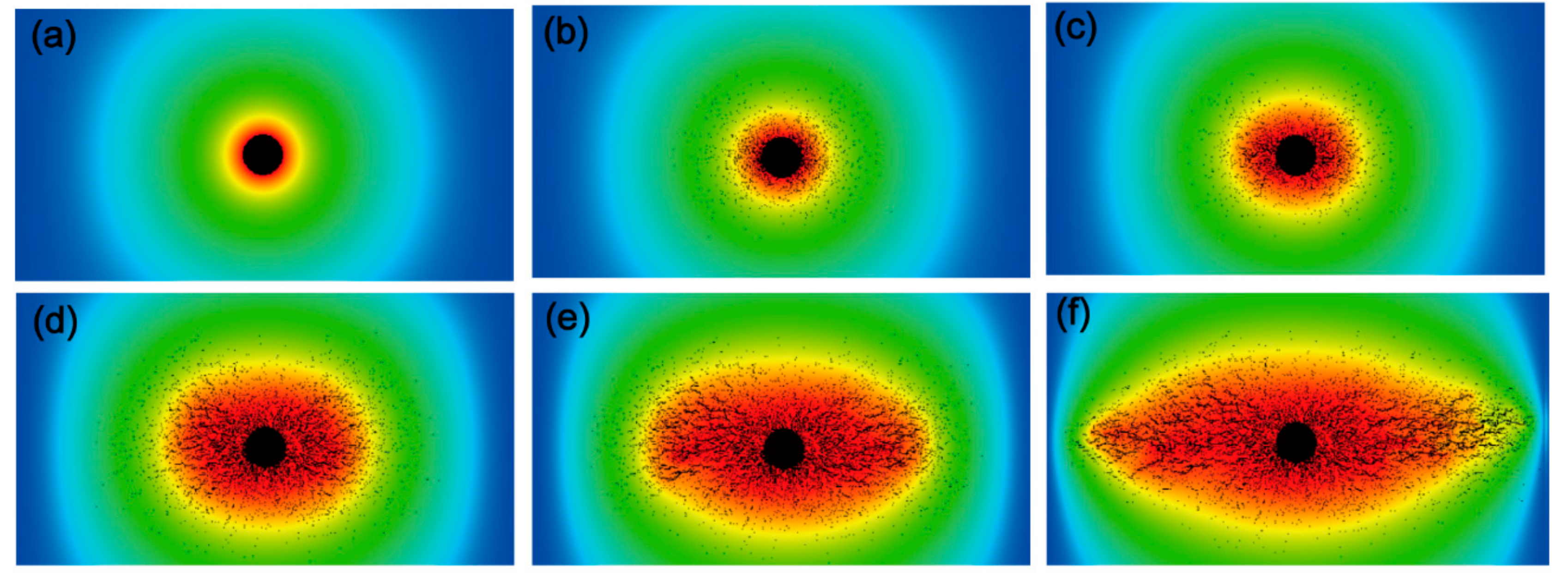
5.1. Effect of In-Situ Stress Ratio

The in-situ stresses in a reservoir significantly affect the performance of hydraulic fracturing [26,50]. The stress ratio, which is defined as the ratio of σ_H/σ_h, was studied to evaluate its effect on the response to fluid injection during hydraulic fracturing.

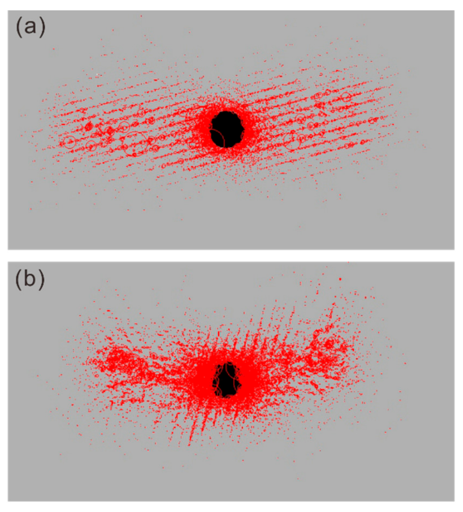
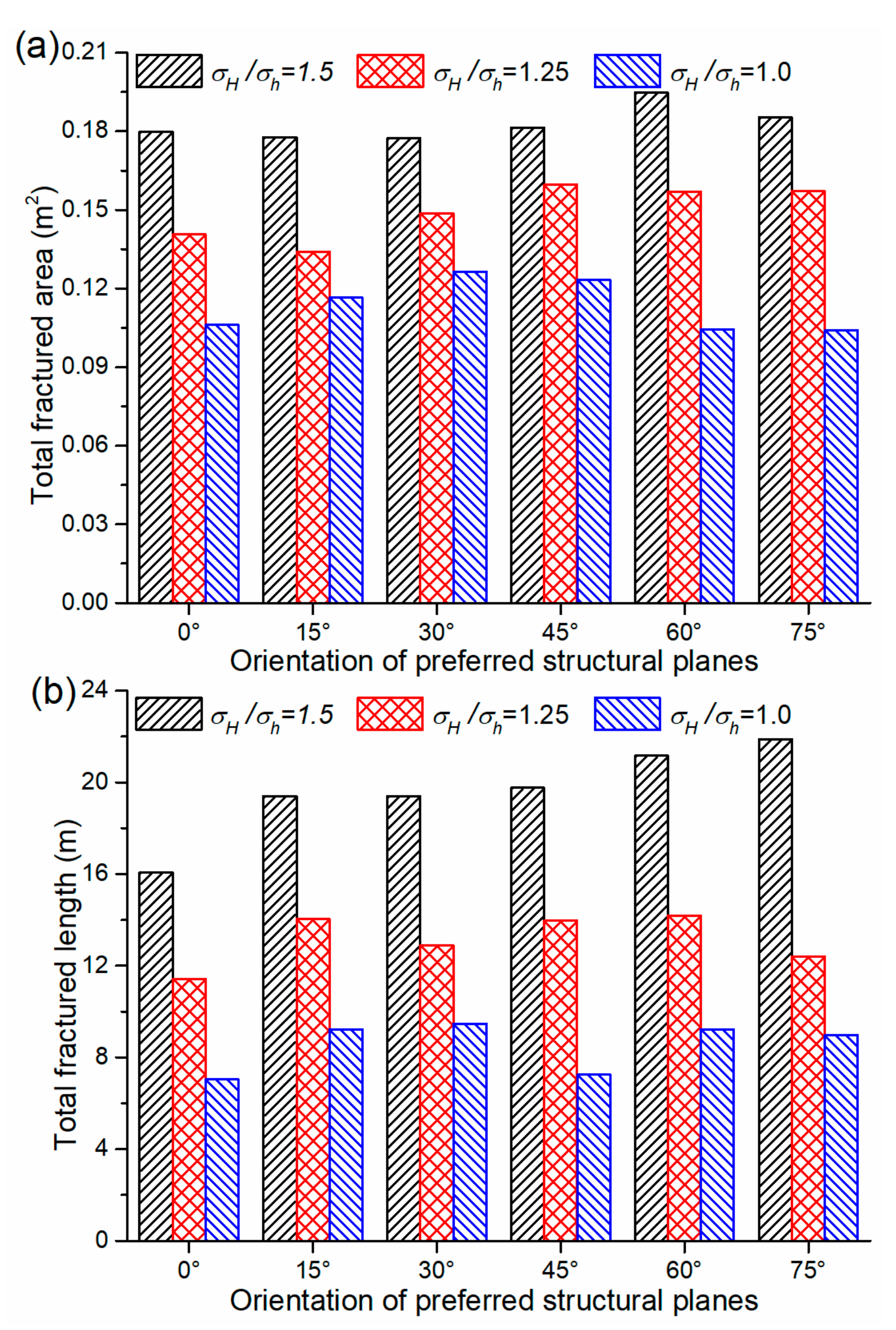
Figure 8 shows the simulated fracture networks with stress ratios equal to 1.5, 1.25, and 1.0. The fracture network zone decreases in size as the stress ratio approaches unity. In addition, the simulation results indicate that the orientation of the long axis of the fractured zone also changes with different stress ratios. Specifically, when the stress ratio equals 1.0, the direction of the fracture zone is about 70° to σ_H; when the stress ratio equals 1.25, the direction of the fracture zone is about 45° to the maximum horizontal stress; and when the stress ratio equals 1.5, the direction of the fracture zone is about 20° to σ_H. In addition, the simulation results show that a large stress ratio is conducive to the development of relatively more branching fractures in the direction of σ_H, which can enhance the connectivity of the hydraulic fractures and add to the complexity of the fracture network morphology.

Figure 9 shows the impact of the stress ratio on the hydraulically fractured area and the length of fractures. The results indicate that the fracture pattern is significantly affected by the stress ratio. For the same injection rate and duration, a higher stress ratio achieves a larger number of simulated fractures and a larger fractured area.

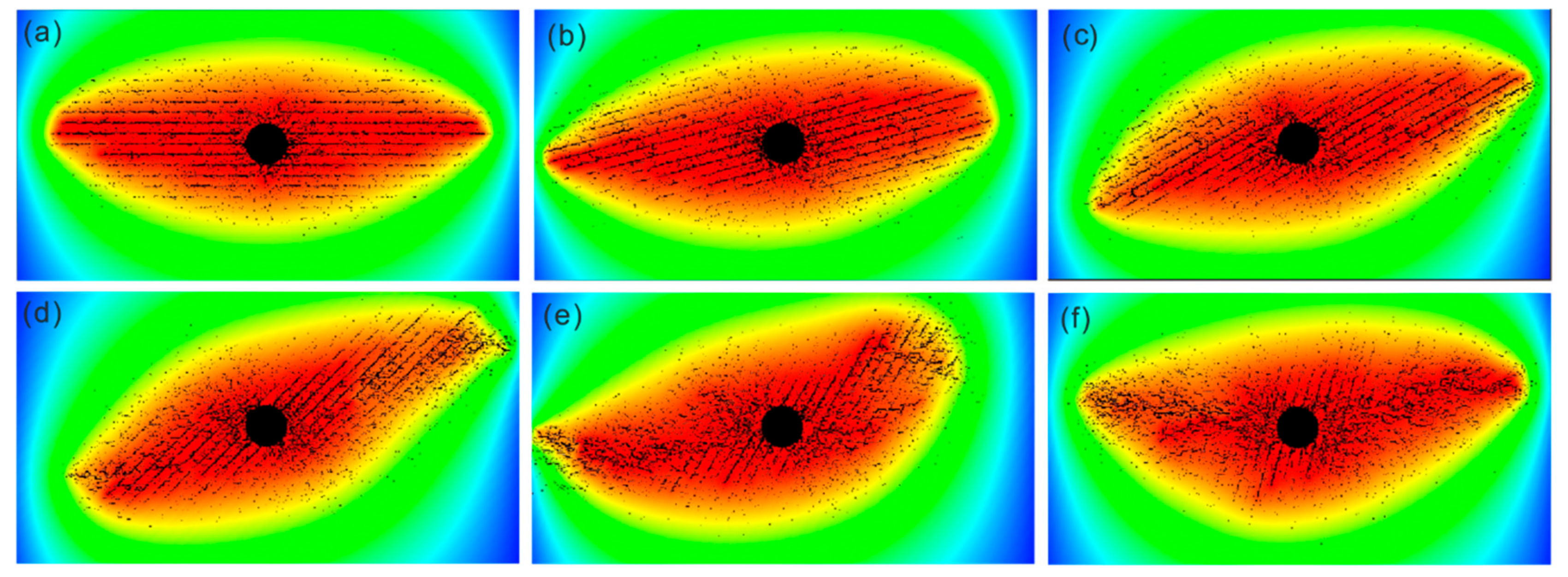
5.2. Effect of Structural Plane Mechanical Properties

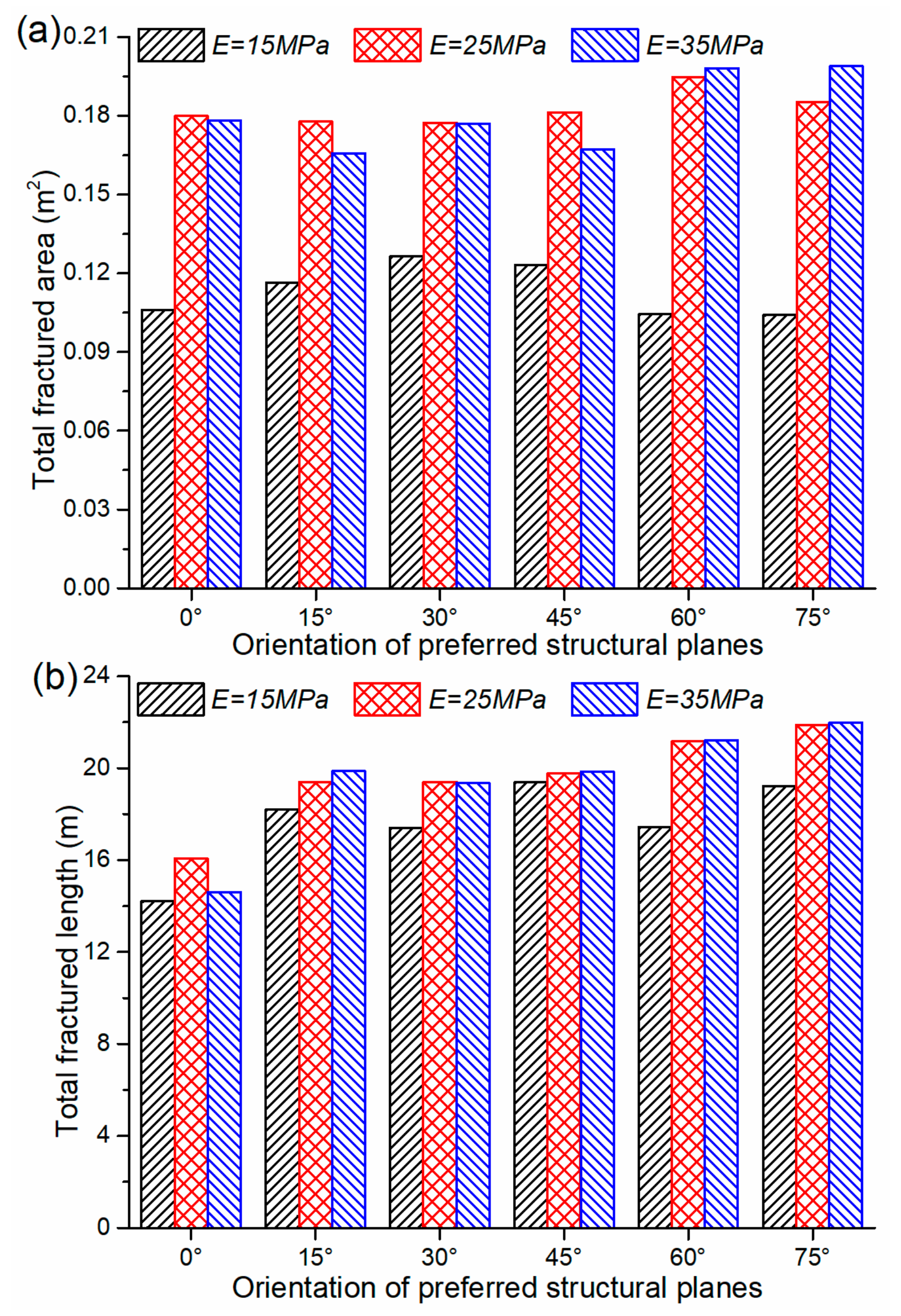
It is generally known that the properties of joints or bedding planes have a significant impact on the deformation and failure behavior of a rock mass. In shale fracturing, the mechanical properties of the structural planes represent an important issue, which cannot be ignored in the design of hydraulic fracturing. The structural planes in the numerical models are elements with lower mechanical properties than the rock matrix. Different elastic moduli of structural planes were assigned to the models to evaluate the effect of the stiffness and strength of the structural planes on the hydraulic fracturing. Figure 10 shows the quantitative results of the simulated fracture network when the structural planes have different elasticity moduli. The fractured area and length of fractures changed slightly with an increase of the elastic modulus of structural planes, which were 30%, 50%, and 70% of the rock matrix, respectively. There was no significant change in the morphology of the fractured zone with an increase of elasticity moduli.

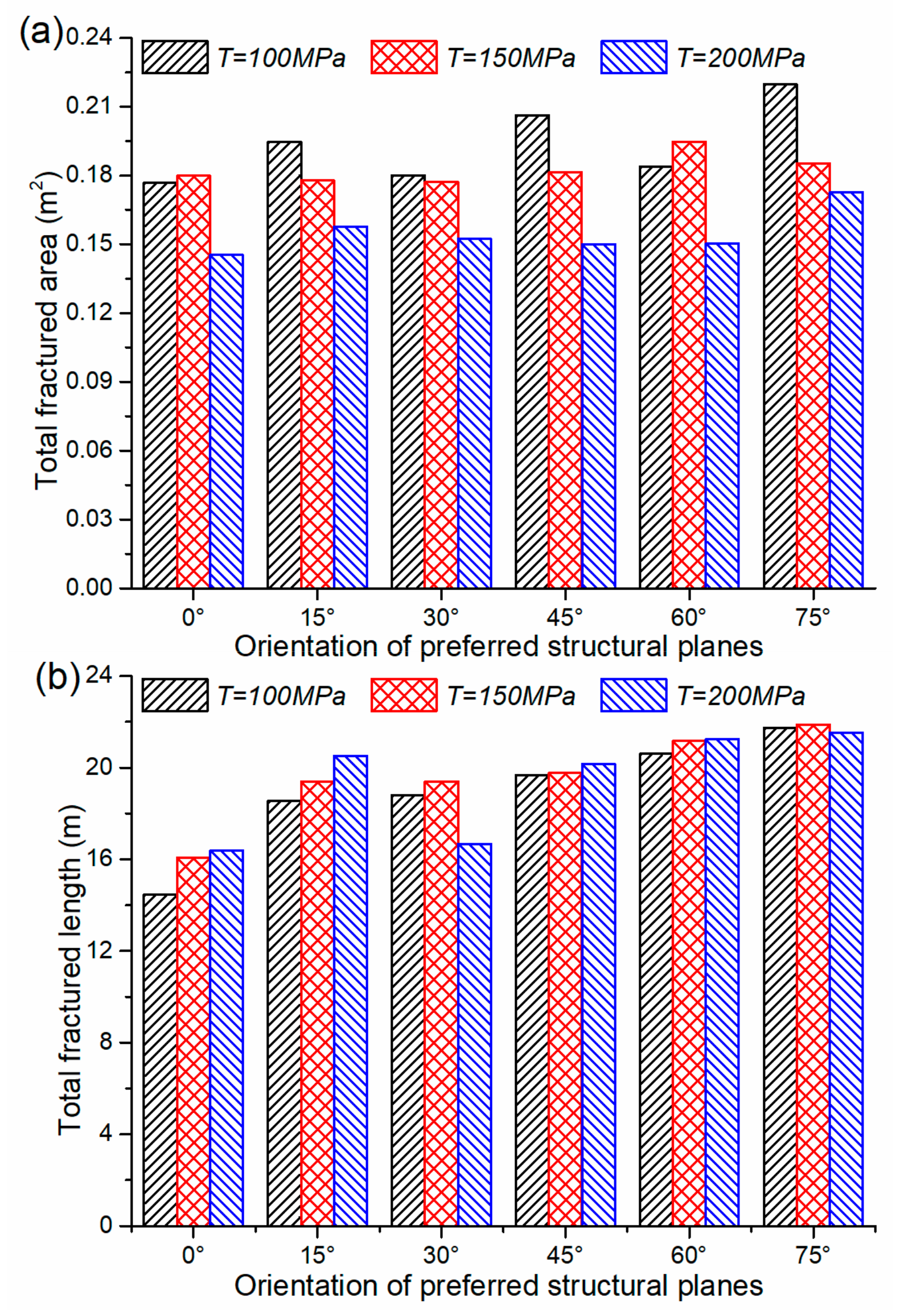
Figure 11 shows the fractured area and length of fractures when the structural planes have different uniaxial compressive strengths. The default tensile-compression strength ratio of material in the FSD is 10. Therefore, changes in the uniaxial compressive strength of the structural planes are essentially paired with changes in the tensile strength in this study. The results suggest that the fractured area increases with a reduction in the uniaxial compressive strength of the structural planes, but the length of fractures in the fracture network decreases.

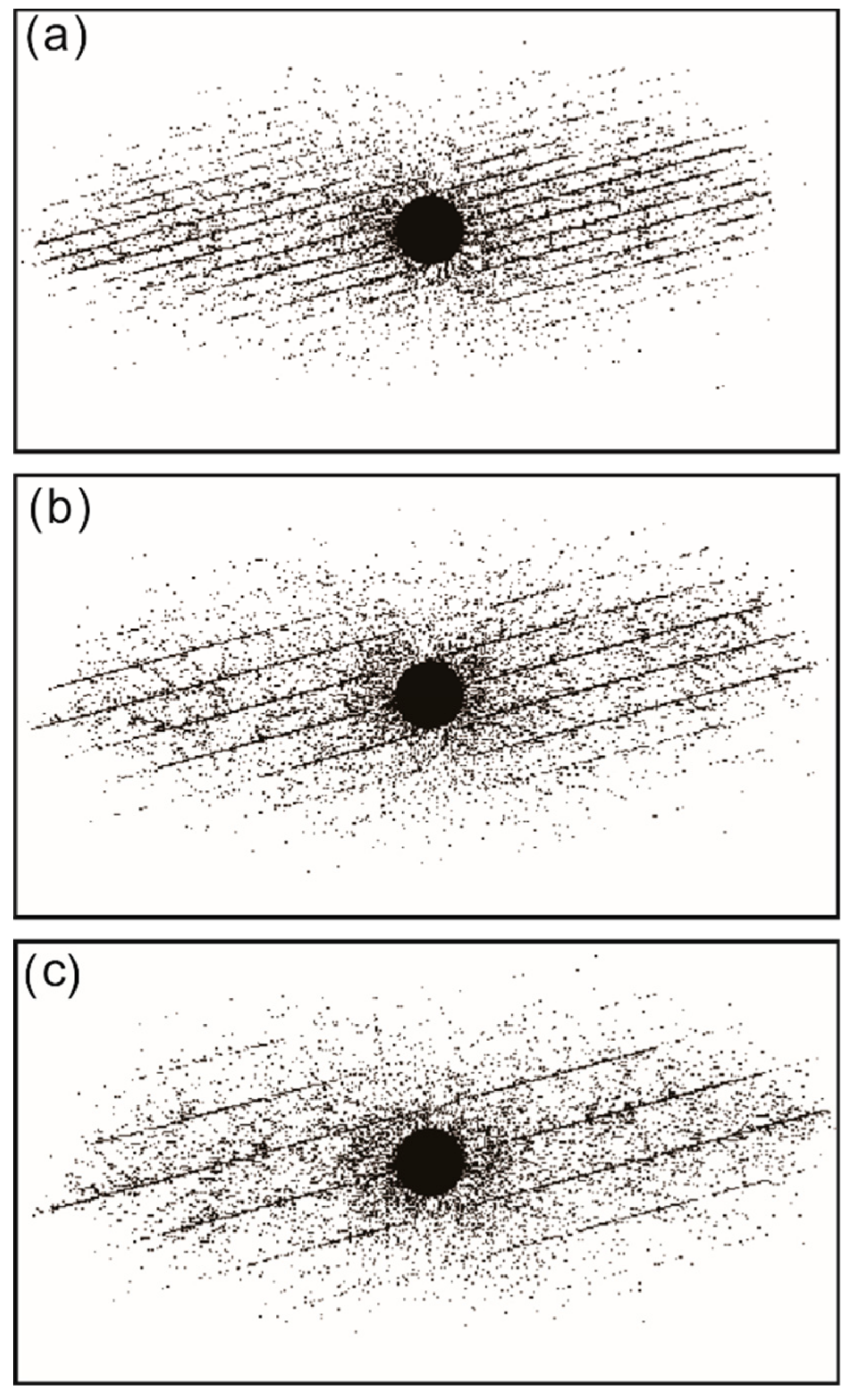
Figure 12 shows the qualitative results of the simulated fracture network when the structural planes have different compressive strengths. The strength of the structural planes has an important influence on hydraulic fracturing. At a strength of 100 MPa, the hydraulic fractures initiated and propagated rapidly along the weak structural planes, and only a few small branching fractures were induced between the main hydraulic fractures, resulting in poor connectivity of the fracture network. At a strength of 150 MPa, although the zone of failed structural planes is smaller than the former case, there are more branching fractures between the structural planes. In this case, the structural planes still dominated the evolution of hydraulic fractures. At a strength of 200 MPa, which is very close to the strength of the rock matrix, the morphology of the fracture network is distinctly different. Here, the impact of the structural planes on hydraulic fracturing is not apparent, and the morphology of the fractured zone is similar to the base model.

5.3. Effect of Structural Plane Spacing

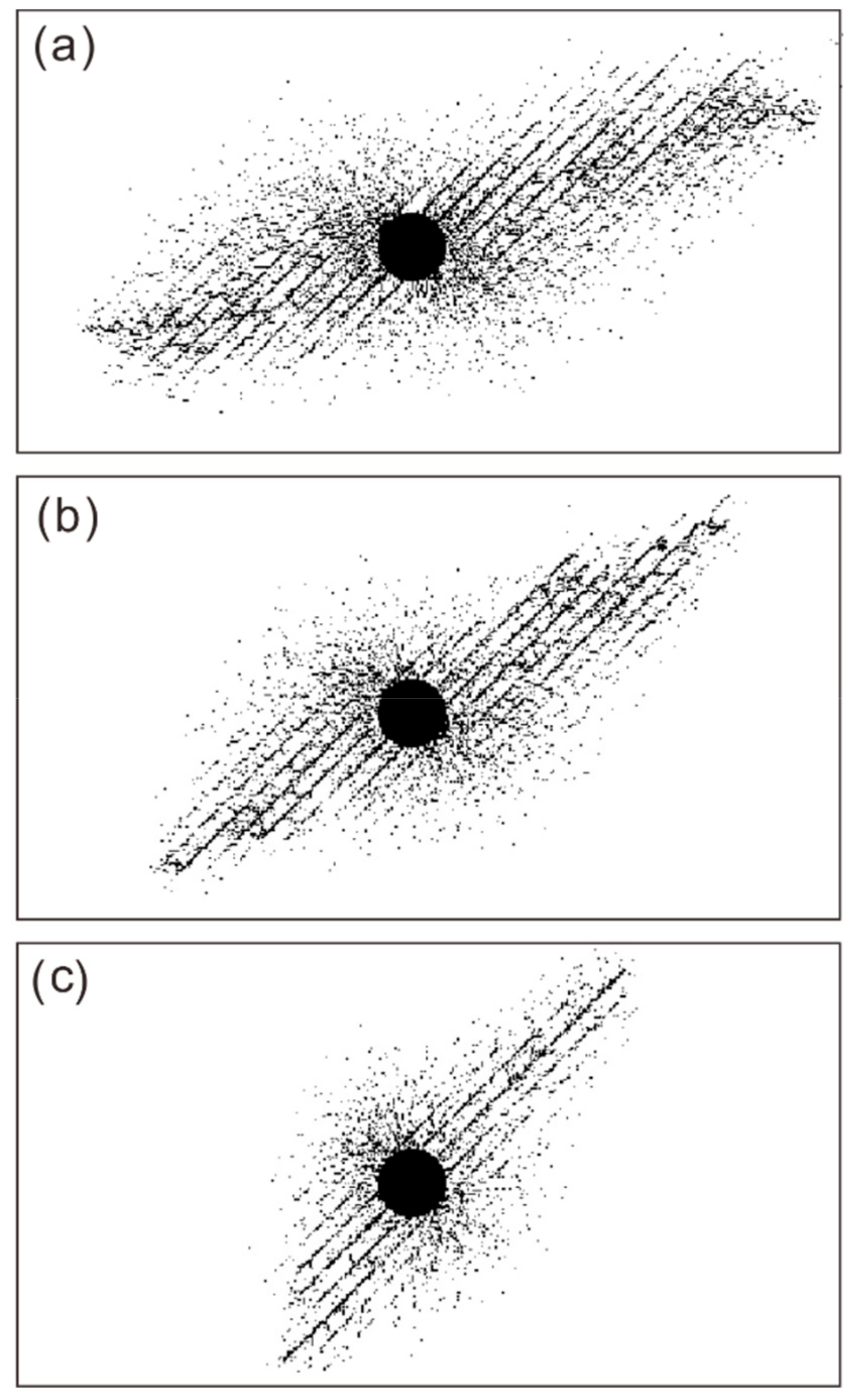
As stated before, natural structural planes typically form a key part of a hydraulic fracture network. Therefore, the structural plane spacing and the number of sets of planes can inevitably affect the morphology of the fracture network and the effectiveness of the hydraulic fracturing. A group of structural planes with different spacings was studied. 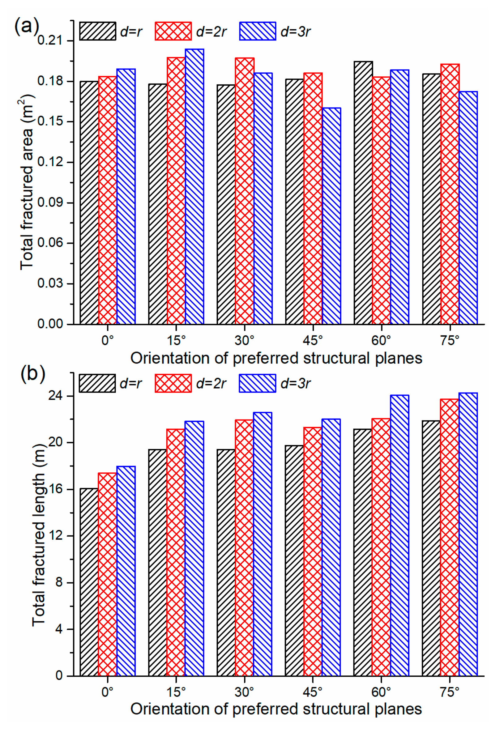For example, with an orientation of the structural planes equal to 15°, Figure 13 shows the distribution of the simulated fracture network when the structural planes have different spacing. The structural plane spacing influences the morphology and connectivity of the fracture network. The failed structural planes dominate the development of the hydraulic fractures and control the pattern of the fracture network. Simulation results with a smaller spacing generate more complex fracture networks and better fracture connectivity. Figure 14 shows the fractured area and the total length of fractures for structural plane spacings of 1, 2, and 3 times the radius of the injection hole. The fractured area did not vary significantly for different spacings, but a reduction in spacing resulted in a decrease in the total length of fractures that were created.

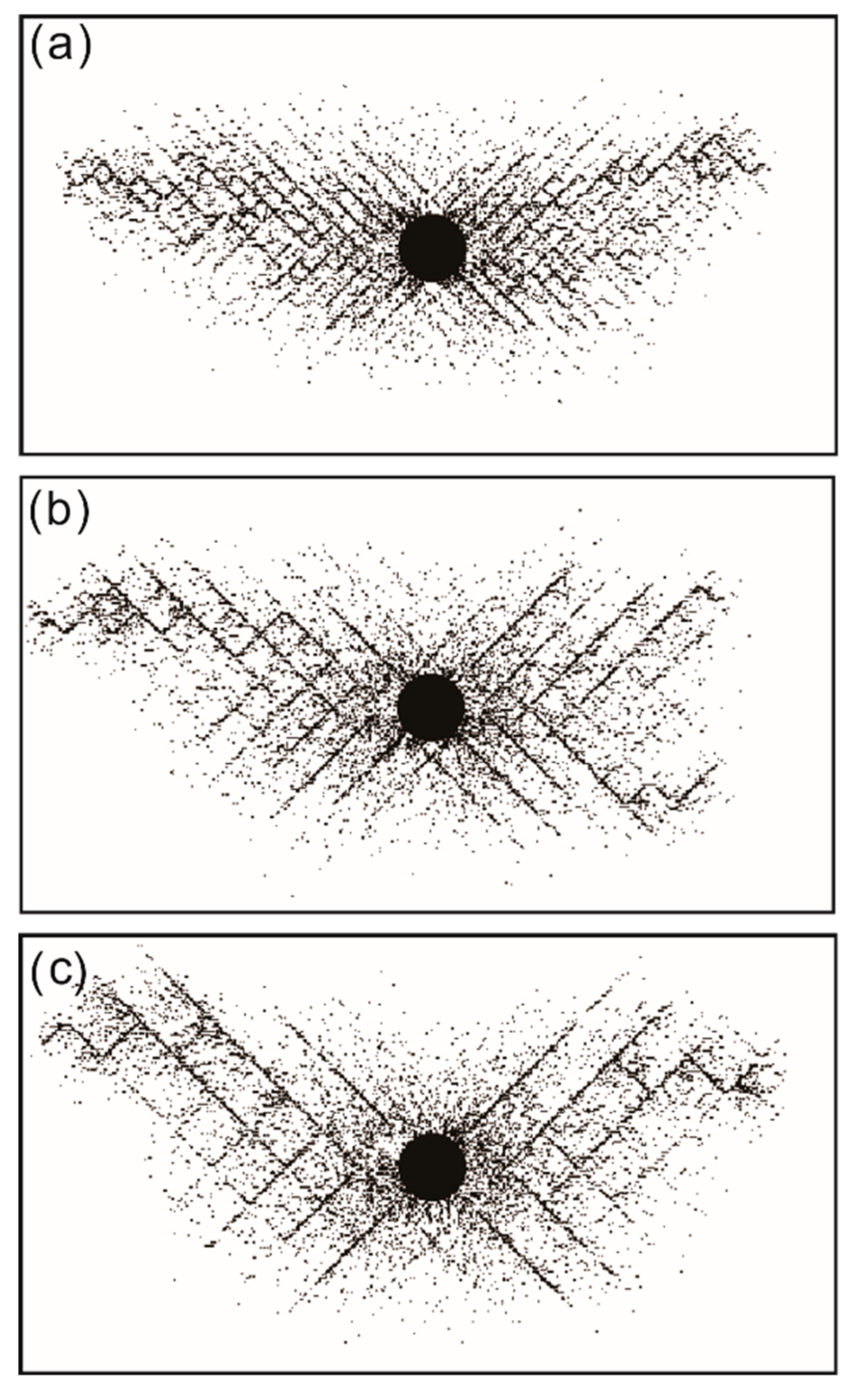
There may be multiple sets of structural planes in a reservoir. To study this more complex geological condition, the effect of the structural plane spacing on the hydraulic fracturing for two sets of weakness planes was also simulated. Figure 15 shows the qualitative characteristics of the simulated fracture networks for two sets of orthogonal structural planes with different spacings. In this case, the structural planes still dominated the morphology and connectivity of the fracture network. Although the model with wider spacing for the structural planes achieved a larger fractured area, it had fewer hydraulic fractures and poor connectivity compared to the model with closer spacing.

5.4. Effect of Injection Rates

The injection rate is one of the most important operational parameters when conducting hydraulic fracturing in shales [3,5]. Although it was believed that large injection rates can enhance the propagation length of fractures [8], the quantitative relationship between the injection rate and the reservoir fracturing is still largely unknown [4]. In this study, different injection rates were tested to study their effects on hydraulic fracturing.

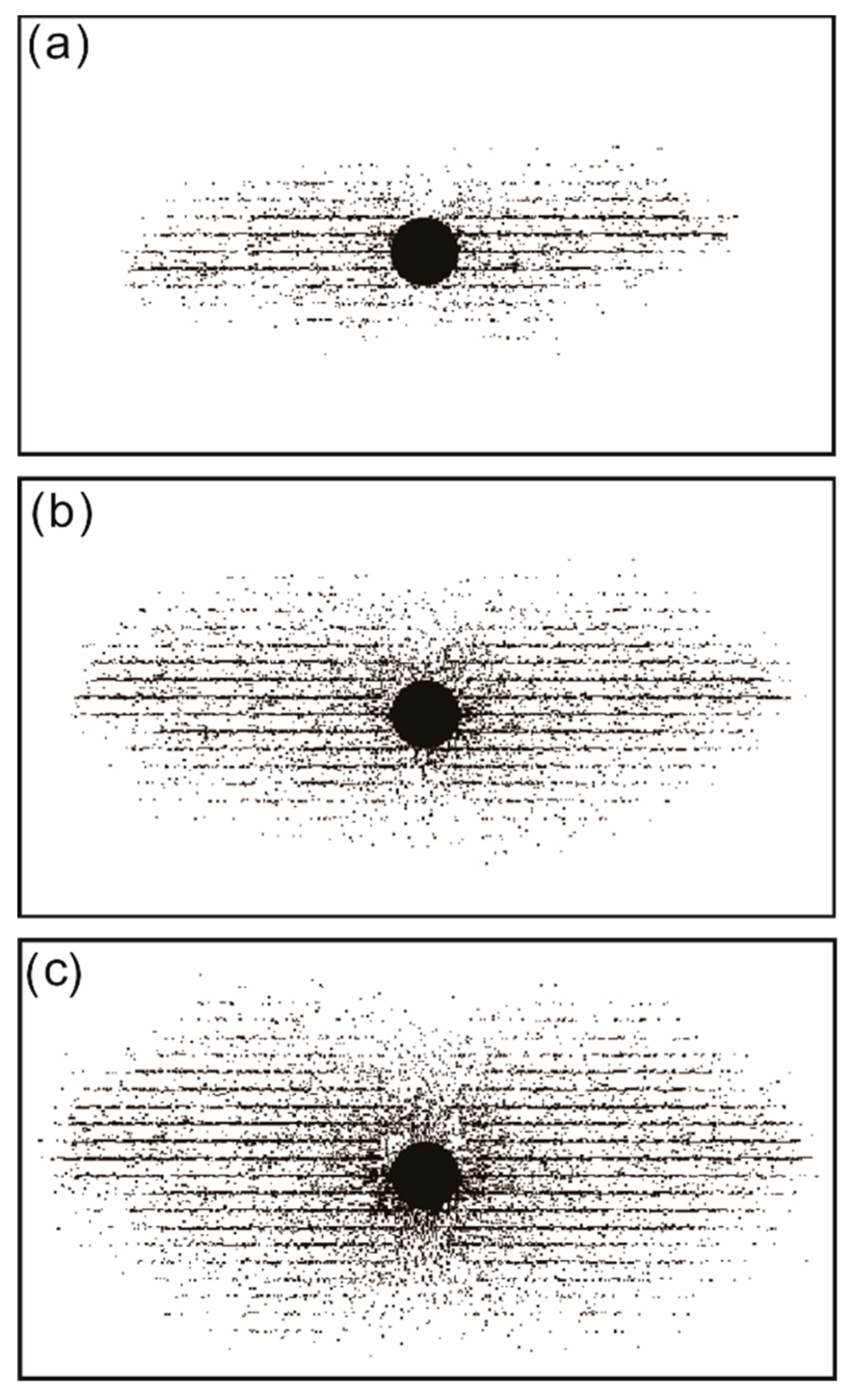
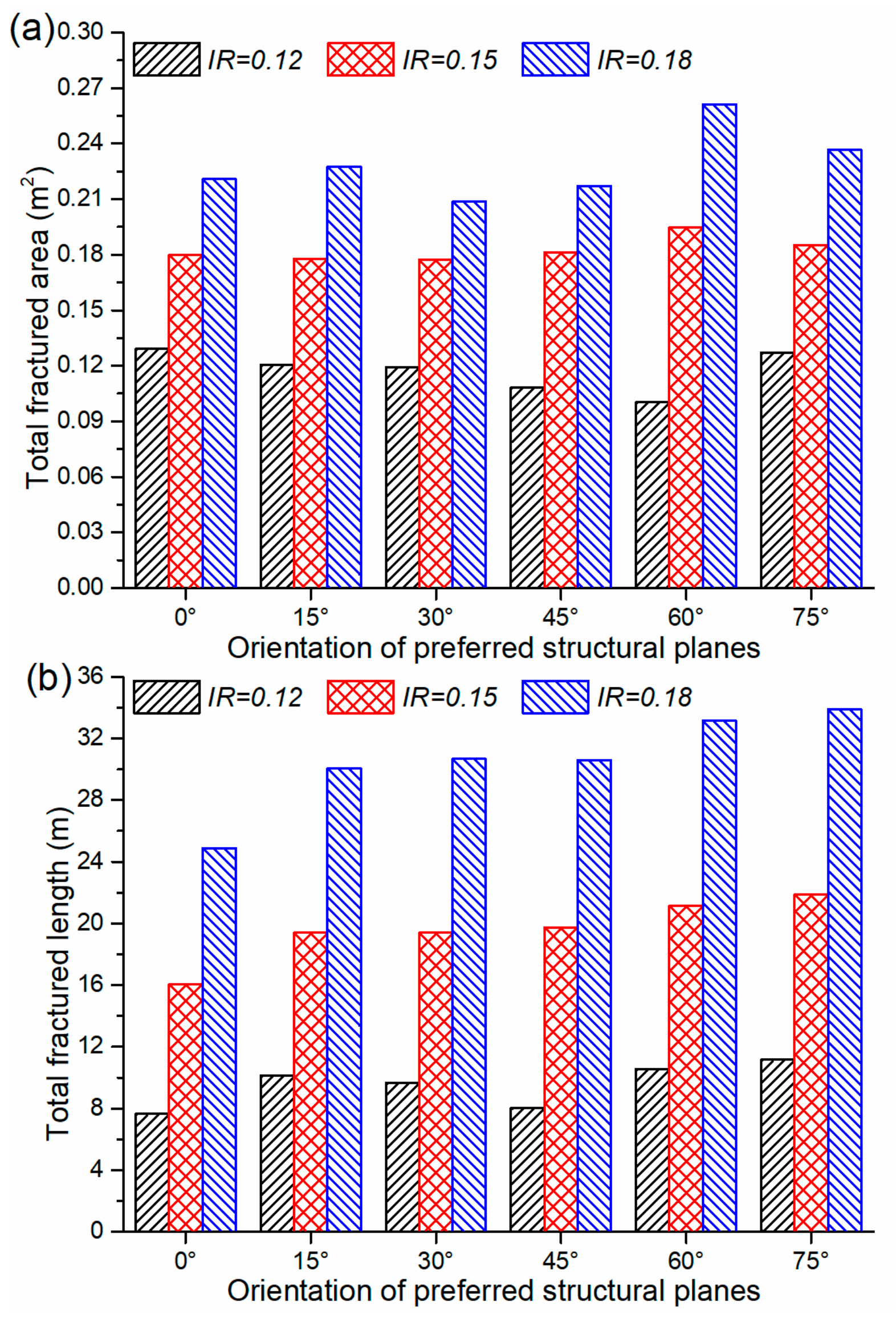
Figure 16 shows the qualitative results of the simulated fracture network with injection rates equal to 0.12, 0.15, and 0.18 m³·s⁻¹·m⁻¹, with the structural planes parallel to σ_H. The injection rate affects the growth and development of the fracture network during the hydraulic fracturing. High injection rates create a larger fractured area and a longer total fracture length. The fractured area and number of fractures increased with the injection rate. For a high injection rate, the injection fluids not only fracture the structural planes, but also initiate small fractures in the rock matrix. In contrast, for a lower injection rate, the time required to reach the breakdown pressure of the shale may be longer, thus resulting in less fractured structural planes and high rates of fluid leak-off into the formation.

Figure 17 shows the quantitative results of the fractured area and length for different constant injection rates. The results show that higher injection rates result in better hydraulic fracturing. At a low injection rate, the fracturing fluid tends to only flow along the structural planes in the direction of σ_H. However, at a high injection rate, multiple random branches of hydraulic fractures form, creating a more complex and connected fracture network.

6. Conclusions

The evolution of hydraulic fracturing in bedding or laminated rocks was investigated through a micromechanics-based 2D numerical modeling approach. The numerical models incorporated heterogeneity in the mechanical properties of the rock and all models other than the base model included planes of weaker elements to simulate the presence of structural features, such as bedding planes in the rock. The mechanical-hydraulic coupled process between the rock and the injected fluid was also incorporated in the models. A series of simulations were conducted to explore the effect of the rock’s mechanical properties and fluid injection rates on the initiation and propagation of fractures and the resulting morphology of the fracture network created.

The process of hydraulic fracturing in laminated rock can be divided into five stages: stress accumulation, small fracture formation, hydraulic fracture initiation, hydraulic fracture propagation, and decay in fracture propagation. Heterogeneity in rock properties influences the fracture initiation and propagation, and the location and orientation of fracture initiation are unpredictable.

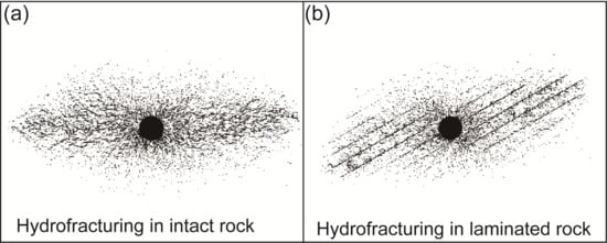
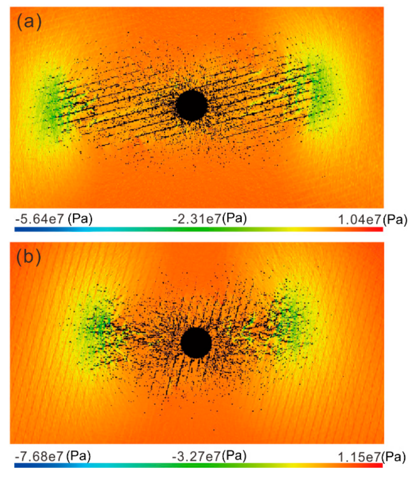
The angle between the orientation of the structural planes and the maximum horizontal stress has a significant effect on the propagation and evolution of the fracture network. When the structural planes are nearly parallel with the direction of σ_H, the weak structural planes dominate the propagation direction and the morphology of the fracture network. When the orientation of the structural planes is significantly different from the direction of σ_H, the extent and morphology of the fracture network are controlled by both the in-situ stresses and the orientation of the structural planes. In this case, many small transverse secondary fractures can occur in conjunction with fracturing along the structural planes. The acoustic emission events induced by the hydraulic fracturing demonstrated that most of the failed elements are caused by tensile failure at the microscale.

The in-situ stress ratio has a great impact on the morphology and extent of the fracture network. For a fixed injection rate and duration, a high-stress ratio creates a larger area of fractured rock with a better connectivity. The stiffness of the structural planes has minimal influence on the extent and morphology of the fracture network, but the mechanical strength of pre-existing weakness planes, the plane spacing, and the injection rate have a significant effect on the hydraulic fracturing. Small structural plane spacing, a high strength contrast, a high-stress ratio, and a high injection rate result in a complex interconnected network of hydraulic fractures.

References

1. Bunger, P.A.; McLennan, J.; Jeffrey, R. Effective and Sustainable Hydraulic Fracturing; InTech: Rijeka, Croatia, 2013. [Google Scholar]
2. Cipolla, C.L.; Warpinski, N.R.; Mayerhofer, M.J. Hydraulic fracture complexity: Diagnosis, remediation, and exploitation. In Proceedings of the SPE Asia Pacific Oil and Gas Conference and Exhibition, Perth, WA, Australia, 24–25 October 2008. [Google Scholar]
3. Gale, J.F.W.; Read, J.M.; Holder, J. Natural fractures in the Barnett shale and their importance for hydraulic fracture treatments. AAPG Bull. 2007, 91, 603–622. [Google Scholar] [CrossRef]
4. He, J.M.; Lin, C.; Li, X.; Wan, X.L. Experimental investigation of crack extension patterns in hydraulic fracturing with shale, sandstone and granite cores. Energies 2016, 9, 1018. [Google Scholar] [CrossRef]
5. Zhou, J.; Chen, M.; Jin, Y.; Zhang, G.Q. Analysis of fracture propagation behavior and fracture geometry using a tri-axial fracturing system in naturally fractured reservoirs. Int. J. Rock Mech. Min. 2008, 45, 1143–1152. [Google Scholar] [CrossRef]
6. Li, X.; Feng, Z.; Han, G.; Elsworth, D.; Marone, C.; Saffer, D. Hydraulic fracturing in shale with H2O, CO2 and N2. In Proceedings of the 49th US Rock Mechanics/Geomechanics Symposium, San Francisco, CA, USA, 28 June–1 July 2015. [Google Scholar]
7. Guo, T.; Zhang, S.; Qu, Z. Experimental study of hydraulic fracturing for shale by stimulated reservoir volume. Fuel 2014, 128, 373–380. [Google Scholar] [CrossRef]
8. Gale, J.F.W.; Laubach, S.E.; Olson, J.E.; Eichhubl, P.; Fall, A. Natural fractures in shale: A review and new observations. AAPG Bull. 2014, 98, 2165–2216. [Google Scholar] [CrossRef]
9. Zhang, C.L.; Armand, G.; Conil, N.; Laurich, B. Investigation on anisotropy of mechanical properties of Callovo-Oxfordian claystone. Eng. Geol. 2019, 251, 128–145. [Google Scholar] [CrossRef]
10. Valente, S.; Fidelibus, C.; Loew, S.; Cravero, M.; Iabichino, G.; Barpi, F. Analysis of Fracture Mechanics Tests on Opalinus Clay. Rock Mech. Rock Eng. 2012, 45, 767–779. [Google Scholar] [CrossRef] [Green Version]
11. Kakouris, E.G.; Triantafyllou, S.P. Material point method for crack propagation in anisotropic media: A phase field approach. Arch. Appl. Mech. 2018, 88, 287–316. [Google Scholar] [CrossRef]
12. Bleyer, J.; Alessi, R. Phase-field modeling of anisotropic brittle fracture including several damage mechanisms. Comput. Method. Appl. M. 2018, 336, 213–236. [Google Scholar] [CrossRef] [Green Version]
13. Amadei, B. Importance of anisotropy when estimating and measuring in-situ stresses in rock. Int. J. Rock. Mech. Min. Sci. Geomech. Abstr. 1996, 33, 293–325. [Google Scholar] [CrossRef]
14. Davies, R.J.; Mathias, S.A.; Moss, J.; Hustoft, S.; Newport, L. Hydraulic fractures: How far can they go? Mar. Petrol. Geol. 2012, 37, 1–6. [Google Scholar] [CrossRef] [Green Version]
15. Eshiet, K.I.; Sheng, Y.; Ye, J. Microscopic modelling of the hydraulic fracturing process. Environ. Earth Sci. 2013, 68, 1169–1186. [Google Scholar] [CrossRef]
16. Frohlich, C. Two-year survey comparing earthquake activity and injection-well locations in the Barnett Shale, Texas. PANS 2012, 109, 13934–13938. [Google Scholar] [CrossRef] [Green Version]
17. Warpinski, N.R.; Teufel, L.W. Influence of geologic discontinuities on hydraulic fracture propagation. J. Pet. Technol. 1984, 39, 209–220. [Google Scholar] [CrossRef]
18. Olson, J.E.; Bahorich, B.; Holder, J. Examining hydraulic fracture: Natural fracture interaction in hydrostone block experiments. In Proceedings of the Society of Petroleum Engineers (SPE) Hydraulic Fracturing Technology Conference, The Woodlands, TX, USA, 6–8 February 2012. [Google Scholar] [CrossRef]
19. Dehghan, N.A.; Goshtasbi, K.; Ahangari, K.; Jin, Y. The effect of natural fracture dip and strike on hydraulic fracture propagation. Int. J. Rock Mech. Min. Sci. 2015, 75, 210–215. [Google Scholar] [CrossRef]
20. Zhao, H.J.; Ma, F.S.; Liu, G.; Feng, X.L.; Guo, J. Analytical investigation of hydraulic fracture-induced seismicity and fault activation. Environ. Earth Sci. 2018, 77, 526. [Google Scholar] [CrossRef]
21. Fu, P.C.; Johnson, S.M.; Carrigan, C.R. An explicitly coupled hydro-geomechanical model for simulating hydraulic fracturing in arbitrary discrete fracture networks. Int. J. Numer. Anal. Methods Geomech. 2013, 37, 2278–2300. [Google Scholar] [CrossRef]
22. Rahman, M.M.; Rahman, S.S. Studies of hydraulic fracture-propagation behavior in presence of natural fractures: Fully coupled fractured-reservoir modeling in poroelastic environments. Int. J. Geomech. 2013, 13, 809–826. [Google Scholar] [CrossRef]
23. Rabczuk, T.; Belytschko, T. Cracking particles: A simplified meshfree method for arbitrary evolving cracks. Int. J. Numer. Methods Eng. 2004, 61, 2316–2343. [Google Scholar] [CrossRef]
24. Wang, S.; Sun, L.; Au, A.; Yang, T.; Tang, C. 2D-numerical analysis of hydraulic fracturing in heterogeneous geo-materials. Constr. Build. Mater. 2009, 23, 2196–2206. [Google Scholar] [CrossRef]
25. Yoon, J.S.; Zimmermann, G.; Zang, A. Numerical investigation on stress shadowing in fluid injection-induced fracture propagation in naturally fractured geothermal reservoirs. Rock Mech. Rock Eng. 2015, 48, 1439–1454. [Google Scholar] [CrossRef]
26. Zhou, J.; Zhang, L.Q.; Braun, A.; Han, Z.H. Numerical modeling and investigation of fluid-driven fracture propagation in reservoirs based on a modified fluid-mechanically coupled model in two-dimensional particle flow code. Energies 2016, 9, 699. [Google Scholar] [CrossRef]
27. Mohammadnejad, T.; Khoei, A.R. An extended finite element method for fluid flow in partially saturated porous media with weak discontinuities; the convergence analysis of local enrichment strategies. Comput. Mech. 2013, 51, 327–345. [Google Scholar] [CrossRef]
28. Cho, N.; Martin, C.D.; Sego, D.C. A clumped particle model for rock. Int. J. Rock Mech. Min. Sci. 2007, 44, 997–1010. [Google Scholar] [CrossRef]
29. Miehe, C.; Mauthe, S. Phase field modeling of fracture in multi-physics problems. Part III. Crack driving forces in hydro-poro-elasticity and hydraulic fracturing of fluid-saturated porous media. Comput. Method. Appl. M. 2016, 304, 619–655. [Google Scholar] [CrossRef]
30. Wilson, Z.A.; Landis, C.M. Phase-field modeling of hydraulic fracture. J. Mech. Phys. Solids 2016, 96, 264–290. [Google Scholar] [CrossRef] [Green Version]
31. Ehlers, W.; Luo, C.A. A phase-field approach embedded in the theory of porous media for the description of dynamic hydraulic fracturing. Comput. Method. Appl. Mech. Eng. 2017, 315, 348–368. [Google Scholar] [CrossRef]
32. Tang, H.Y.; Li, S.B.; Zhang, D.X. The effect of heterogeneity on hydraulic fracturing in shale. J. Petrol. Sci. Eng. 2018, 162, 292–308. [Google Scholar] [CrossRef]
33. Yang, T.H.; Tham, L.G.; Tang, C.A.; Liang, Z.Z.; Tsui, Y. Influence of heterogeneity of mechanical properties on hydraulic fracturing in permeable rocks. Rock Mech. Rock Eng. 2004, 37, 251–275. [Google Scholar] [CrossRef]
34. Lan, H.X.; Martin, C.D.; Hu, B. Effect of heterogeneity of brittle rock on micromechanical extensile behavior during compression loading. J. Geophys. Res. Sol. Earth 2010, 115, B01202. [Google Scholar] [CrossRef]
35. Ishida, T.; Chen, Q.; Mizuta, Y.; Roegiers, J.C. Influence of fluid viscosity on the hydraulic fracturing mechanism. J. Energy Resour. Technol. 2004, 126, 190–200. [Google Scholar] [CrossRef]
36. Shimizu, H.; Murata, S.; Ishida, T. The distinct element analysis for hydraulic fracturing in hard rock considering fluid viscosity and particle size distribution. Int. J. Rock Mech. Min. Sci. 2011, 48, 712–727. [Google Scholar] [CrossRef]
37. Hou, B.; Chen, M.; Li, Z.M. Propagation area evaluation of hydraulic fracture networks in shale gas reservoirs. Pet. Explor. Dev. 2014, 41, 833–838. [Google Scholar] [CrossRef]
38. Tang, C.A. Numerical simulation of progressive rock failure and associated seismicity. Int. J. Rock. Mech. Min. Sci. 1997, 34, 249–261. [Google Scholar] [CrossRef]
39. Tang, C.A.; Tham, L.G.; Lee, P.K.K. Coupled analysis of flow, stress and damage (FSD) in rock failure. Int. J. Rock. Mech. Min. Sci. 2002, 39, 477–489. [Google Scholar] [CrossRef]
40. Tang, C.A.; Xu, X.H.; Zhao, W.; Yang, W.T. A new approach to numerical method of modelling geological processes and rock engineering problems. Eng. Geol. 1998, 49, 207–214. [Google Scholar] [CrossRef]
41. Tang, C.A.; Liu, H.; Lee, P.K.K.; Tsui, Y.; Tham, L.G. Numerical studies of the influence of microstructure on rock failure in uniaxial compression—Part I: Effect of heterogeneity. Int. J. Rock Mech. Min. Sci. 2000, 37, 555–569. [Google Scholar] [CrossRef]
42. Tang, C.A.; Tham, L.G.; Lee, P.K.K.; Tsui, Y.; Liu, H. Numerical studies of the influence of microstructure on rock failure in uniaxial compression—Part II: Constraint, slenderness and size effects. Int. J. Rock Mech. Min. Sci. 2000, 37, 570–577. [Google Scholar] [CrossRef]
43. Sharif, M.N.; Islam, M.N. The Weibull distribution as a general model for forecasting technological change. Technol. Forecast. Soc. 1980, 18, 247–256. [Google Scholar] [CrossRef]
44. Wang, Y.; Li, X.; Zhou, R.Q.; Zheng, B.; Zhang, B.; Wu, Y.F. Numerical evaluation of the effect of fracture network connectivity in naturally fractured shale based on FSD model. Sci. China Earth Sci. 2015, 58, 1–14. [Google Scholar] [CrossRef]
45. Liu, Z.; Chen, M.; Zhang, G. Analysis of the Influence of a Natural Fracture Network on Hydraulic Fracture Propagation in Carbonate Formations. Rock Mech. Rock Eng. 2013, 47, 575–587. [Google Scholar] [CrossRef]
46. He, J.M.; Zhang, Z.B.; Li, X. Numerical analysis on the formation of fracture network during the hydraulic fracturing of shale with pre-existing fractures. Energies 2017, 10, 736. [Google Scholar] [CrossRef]
47. Zhou, J.; Zhang, L.Q.; Pan, Z.J.; Han, Z.H. Numerical investigation of fluid-driven near-borehole fracture propagation in laminated reservoir rock using PFC2D. J. Nat. Gas. Sci. Eng. 2016, 36, 719–733. [Google Scholar] [CrossRef]
48. Ellsworth, W.L. Injection-induced earthquakes. Science 2013, 341. [Google Scholar] [CrossRef] [PubMed]
49. Barton, C.; Moos, D.; Tezuka, K. Geomechanical wellbore imaging: Implications for reservoir fracture permeability. AAPG Bull. 2009, 93, 1551–1569. [Google Scholar] [CrossRef]
50. Nasehi, M.J.; Mortazavi, A. Effects of in-situ stress regime and intact rock strength parameters on the hydraulic fracturing. J. Petrol. Sci. Eng. 2013, 108, 211–221. [Google Scholar] [CrossRef]
Figure 1. Weibull distribution for mechanical properties of materials with different homogeneity indexes m modified from Sharif et al. [43].
Energies 12 03500 g001
Figure 2. Numerical model setup with a plot of modulus distribution showing the bedding orientation at 30° in the model. (a) Geometric model; (b) Numerical model.
Energies 12 03500 g002
Figure 3. Stages of hydraulic fracturing in heterogeneous rock without weakness planes with increasing pore pressure shown by changes in the color; the location of the fractures is shown by the black lines. (a) Initial state; (b) Stress accumulation; (c) Small fracture formation; (d) Hydraulic fracture initiation; (e) Hydraulic fracture propagation; (f) Decay in fracture propagation.
Energies 12 03500 g003
Figure 4. Fracture pattern for bedding orientations of 0°, 15°, 30°, 45°, 60°, and 75°. The color indicates the relative magnitude of the pore water pressure field. The boundary stress and injection rate were the same as the base model. (a) Bedding orientation 0°; (b) Bedding orientation 15°; (c) Bedding orientation 30°; (d) Bedding orientation 45°; (e) Bedding orientation 60°; (f) Bedding orientation 75°.
Energies 12 03500 g004
Figure 5. Hydraulic fractures after hydraulic fracturing of a shale specimen (after Guo et al. (7)).
Energies 12 03500 g005
Figure 6. Distribution of the minor principal stress field after hydraulic fracturing for bedding orientations of 15° and 75°. The boundary stress and injection rate were the same as for the base model. (a) Bedding orientation 15°; (b) Bedding orientation 75°.
Energies 12 03500 g006
Figure 7. Distribution of simulated microseismic events (red circles) during hydraulic fracturing; the circle size indicates the microseismic event magnitude. The bedding orientations are 15° and 75°, and the boundary stress and injection rate were the same as for the base model. (a) Bedding orientation 15°; (b) Bedding orientation 75°.
Energies 12 03500 g007
Figure 8. Fracture distribution for bedding planes oriented at 45°. The in-situ stress ratios were 1.5, 1.25, and 1.0, respectively. The injection rate was consistent with the base model. (a) In-situ stress ratio 1.5; (b) In-situ stress ratio 1.25; (c) in-situ stress ratio 1.0.
Energies 12 03500 g008
Figure 9. Total fractured area (a) and total length of fractures (b) for different in-situ stress ratios. The injection rate was the same as for the base model.
Energies 12 03500 g009
Figure 10. Total fractured area (a) and total length of fractures (b) for different elastic moduli. The boundary stress and injection rate were the same as for the base model.
Energies 12 03500 g010
Figure 11. Total fractured area (a) and total length of fractures (b) for different compressive strengths. The boundary stress and injection rate were the same as with the base model.
Energies 12 03500 g011
Figure 12. Distribution of the fractures for compressive strengths of 100 (a), 150 (b), and 200 MPa (c) for a structural plane orientation of 30°. The boundary stress and injection rate were the same as for the base model.
Energies 12 03500 g012
Figure 13. Distribution of fractures for different structural plane spacings with a structural plane orientation of 15°. The boundary stress and injection rate were the same as with the base model. (a) Bedding spacing is the same as the hole radius (d = r); (b) Bedding spacing is two times of the hole radius (d = 2r); (c) Bedding spacing is two times of the hole radius (d = 3r).
Energies 12 03500 g013
Figure 14. Total fractured area (a) and total length of fractures (b) for different spacings. The boundary stress and injection rate were consistent with the base model.
Energies 12 03500 g014
Figure 15. Failure pattern for models with two orthogonal sets of structural planes with different spacings. The boundary stress and injection rate were the same as with the base model. (a) Bedding spacing is the same as the hole radius (d = r); (b) Bedding spacing is two times of the hole radius (d = 2r); (c) Bedding spacing is two times of the hole radius (d = 3r).
Energies 12 03500 g015
Figure 16. Distribution of the fractures for injection rates of 0.12, 0.15, and 0.18 m3·s−1·m−1 for a case with structural planes parallel to σH and boundary stresses the same as with the base model. (a) Injection rate 0.12 m3·s−1·m−1; (b) Injection rate 0.15 m3·s−1·m−1; (c) Injection rate 0.18 m3·s−1·m−1.
Energies 12 03500 g016
Figure 17. Total fractured area (a) and total length of fractures (b) for different injection rates. The boundary stress was the same as with the base model.
Energies 12 03500 g017