Thermal Effects of Ground Faults on MV Joints and Cables

Abstract

In recent years, an anomalous increase of faults in underground medium voltage (MV) cable lines has been recorded in Italy, especially during summer; the largest number of faults affected cable joints. The assessment of joint thermal stress, both in normal operation and during faults, is paramount. The study presented in this paper focuses on cable heating effects due to short circuit currents flowing through cable screens during ground faults (e.g., in case of cross country faults, CCFs, whose current values are comparable to line-to-line short circuit), considering the contact resistance (CR) between cable screens and copper stocking due to inaccurate joint manufacturing. A thermal model, already developed and discussed by the authors in previous papers, has been extended and applied in this study in order to assess the CR effects in cable and joint heating during failures. Parametric studies have been carried out on a typical cable-joint system, varying fault current and CR values, as well as considering protection schemes normally adopted by distribution system operators (DSOs) in Italian MV distribution grids. Results show that for CR values larger than few milliohms, fault currents due to CCFs are able to overheat the joint well beyond the maximum tolerable temperature of insulation, thus leading to cable failures when the shortest fault clearing times (i.e., 120 ms) are considered.

1. Introduction

In recent years, increasing attention has been paid to faults occurring in cable lines. In 2015, particularly during the month of July, distribution system operators (DSOs) in Italy recorded an abnormal increase of medium voltage (MV) feeder failures, mainly located in cable joints (two to three more frequent compared to previous years). This phenomenon repeated in the subsequent years with varying degrees of intensity.

Recently, Italian DSOs are reporting experiences of joint faults. In [1], Unareti S.p.A. (DSO operating in Milan and Brescia, in the North of Italy) reported wide replacement of joints, substituting those already installed (with a 24 kV rated voltage) with new ones (with a 36 kV rated voltage). As an extreme consequence, authors in [2] proposed redesigning the topology of MV networks in order to reduce the number of joints, since they are considered a weak component. Other works reported the dramatic increasing number of faults occurring within joints, as [3].

Since joints are potential fault hot spots in cable systems [4], some recent works have investigated the physical behavior of cable joints with respect to their thermal aspects. In order to detect internal defects of cable joints, mainly due to low quality construction (e.g., cable eccentricity) and excess contact resistance (CR), reference [5] measured nonuniform temperature distribution in cable joints. Another study [6] presented a model able to obtain the real-time temperature of three-core cable joints under unbalanced three-phase currents and considered the effect of contact resistance in connectors. In [7], an approach for hot spot temperature computation of cable joints was proposed and evaluated by radial basis function neural networks. In such works, however, the influence of CR with respect to cable heating was not quantitatively investigated. References [8,9] mainly focused on the assessment of the influence of CR on cable joint temperature: by using a simplified joint model, a finite element method is presented, showing that CR, in the case of low-quality joints, causes higher temperatures inside the joint with respect to the cable, of about 5 K. In these works, however, only load currents (i.e., current values lower than the cable ampacity) were considered. Moreover, due to the recognized role of CR with respect to cable heating, many papers proposed new methods and models to assess CR in cable joints [10,11,12].

Considering the available literature, very little attention has been paid to the effects of large short circuit currents during transients on MV joint heating. In order to investigate this issue, this paper focused on MV joints’ thermal behavior during severe ground faults, which are able to cause very large current values to flow through the cable screens. Based on the circuit model already developed in [13] and further improved and validated in [14] in order to simulate real cable operations and laying conditions, a full 3D model of the cable-joint system is presented. Differently to [14], the electric CR inside the joint is taken into account. Parametric analyses are carried out by varying the joint CR and by injecting different fault current values; moreover, autoreclosure schemes normally implemented in MV networks by Italian DSOs to provide continuity of supply in case of fault occurrence are considered, in order to accurately reproduce real operating conditions of cable-joint systems.

Section 2 presents the model used to simulate the thermal transients of buried joints, as well as the methodology used to evaluate CR; all parameter values in the simulations are reported. Section 3 describes the autoreclosure schemes commonly implemented by Italian DSOs: different use cases (UCs) are identified and simulated; moreover, Section 3 reports the main results obtained in the simulations, which are finally discussed in Section 4.

2. Materials and Methods

2.1. Thermal Disturbance inside Cables

In this paper, a thermal model including a cable line buried into the ground, cold-shrinkable joints, and the surrounding ground were used in order to evaluate the effects of ground faults on cable heating. Among them, double ground faults, commonly named cross-country faults (CCFs), have been considered, since the related fault currents are high and quite comparable to line-to-line fault currents. In [13], the authors presented a 2D model only considering cable lines and joints, whereas in [14], a full 3D model also including ground was developed, taking into account thermal exchanges between the ground surface and the external environment. In this Section, the authors firstly recall the model described in [14], and then present the method to evaluate the influence of CR inside the joint during thermal transients caused by CCFs.

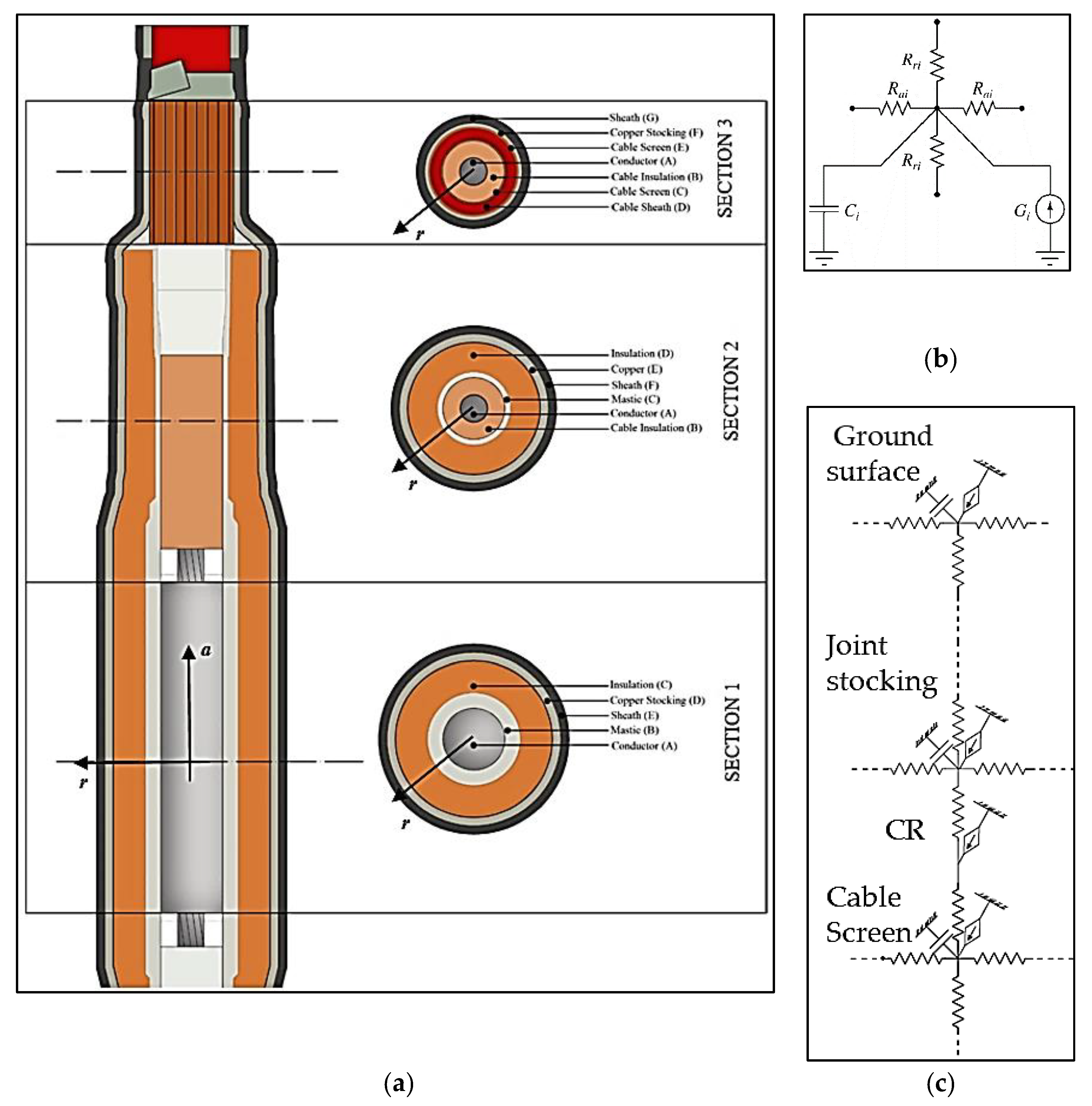
The shape of a cold-shrinkable joint is not straightforward, since it is made up of several parts and materials: a central part, with a conductive connector that joints the cable stretches, normally covered by a two-layer plate and high permittivity mastic layer (MNAC); a triple layer extruded ethylene-propylene diene monomer (EPDM) body, which is the cold-shrinkable part; a copper stocking for continuity of the cable screen; and a protective EPDM sheath.

In order to produce a detailed model, cable and joint have been subdivided in m cylindrical volumes, with m being the number of different materials along the radial direction (r in Figure 1a). The m volumes have been discretized in n equal parts along the axial direction, with n being the fixed discretization step. Each volume is described by means of circuital elements, evaluated according to the Fourier equation:

$$w=-\mathrm{\nabla }\cdot \left(\mathsf{\lambda }\mathrm{\nabla }T\right)+c\frac{\partial T}{\partial t},$$

(1)

where λ is the thermal conductivity, c the volumetric heat capacity, and w the heat source, which depends on temperature T since it is related to the Joule losses of the conductive parts according to the following equation:

$$\mathsf{\rho }(T)={\mathsf{\rho }}_{20°C}\cdot [1+\mathsf{\alpha }(T-20)].$$

(2)

The thermal problem inside the joint and the cable has been solved in polar coordinates: considering the i-th cylindrical elementary volume, the resistive bipoles R_ri and R_ai take into account the thermal resistance along radial and axial directions, respectively. C_i represents the thermal capacity of the volume, whereas G_i is a current generator reproducing the heat source due to Joule losses inside the volume, which depend on the temperature T according to (2). Dielectric losses are negligible, as already demonstrated by the authors in [13].

Quantities R_ri, R_ai, and C_i are evaluated by:

$$\{\begin{array}{l}{R}_{ri}=\frac{1}{2\mathsf{\pi }{\mathsf{\lambda }}_i{L}_i}\ln \frac{r_{e,i}}{r_{i,i}}\\ R_{ai}=\frac{L_i}{\mathsf{\pi }{\mathsf{\lambda }}_i(r_{e,i}^2-r_{i,i}^2)}\\ C_i=\mathsf{\pi }{L}_i{c}_i(r_{e,i}^2-r_{i,i}^2)\end{array}$$

(3)

where λ_i is the thermal conductivity, L_i is the length, r_e,i is the external radius, r_i,i is the internal radius of the i-th cylindrical volume, and c_i is the volumetric heat capacity of the i-th volume. R_ri of copper and aluminum conductors have been neglected. The attendant circuit is reported in Figure 1b. The thermal resistance of the i-th volume between cable and polyvinyl chloride (PVC) pipe, R_i,cp, accounts for the convective, radiating, and conductive heat transfer and has been assessed by means of the empirical formula in [15]:

$$R_{i,cp}=\frac{U}{\left[1+0.1(V+Y{\mathsf{\theta }}_{mi})D_{ei}\right]\cdot L_i}$$

(4)

where U, V, and Y are constants whose values depend on the installation and are reported in [15], ϴ_mi (in °C) is the mean temperature of the air between the cable and the pipe and D_ei (in mm) is the external diameter of the considered volume. If more than one cable is simulated, an empirical coefficient multiplies D_ei in order to take into account the mutual heating between cables in the pipe: according to [15], for three cables grouped in a conduit, the empirical coefficient is equal to 2.15.

Different arrangements are provided by the joint manufacturers (e.g., copper braid or socks mounted with a ring or a weld) in order to ensure screen continuity between the cable stretches; in all of these cases, a CR is introduced in both terminals of the joint.

In the literature, the evaluation of CR is performed by means of either cylindrical volumes, which have their basis as contact sections, or metallic films which are overlapped. The density of contact spots is investigated in [16] and a generalized formula is defined in [17]. Other papers studied the influence of pressure and temperature: experimental tests have demonstrated that contact resistance decreases if pressure and temperature increase, and this correlation is described by nonlinear relationships with hysteresis characteristics, as in [18]. In the present paper, CR’s influence has been taken into account by increasing the locally produced Joule losses, as in [8].

The effect of CR is evaluated, including a specific current generator, in the model, injecting a current equal to the heat flow produced by the Joule losses, as shown in Figure 1c, which is an extract of the whole equivalent network (consisting of about 35,000 nodes) used in the simulations.

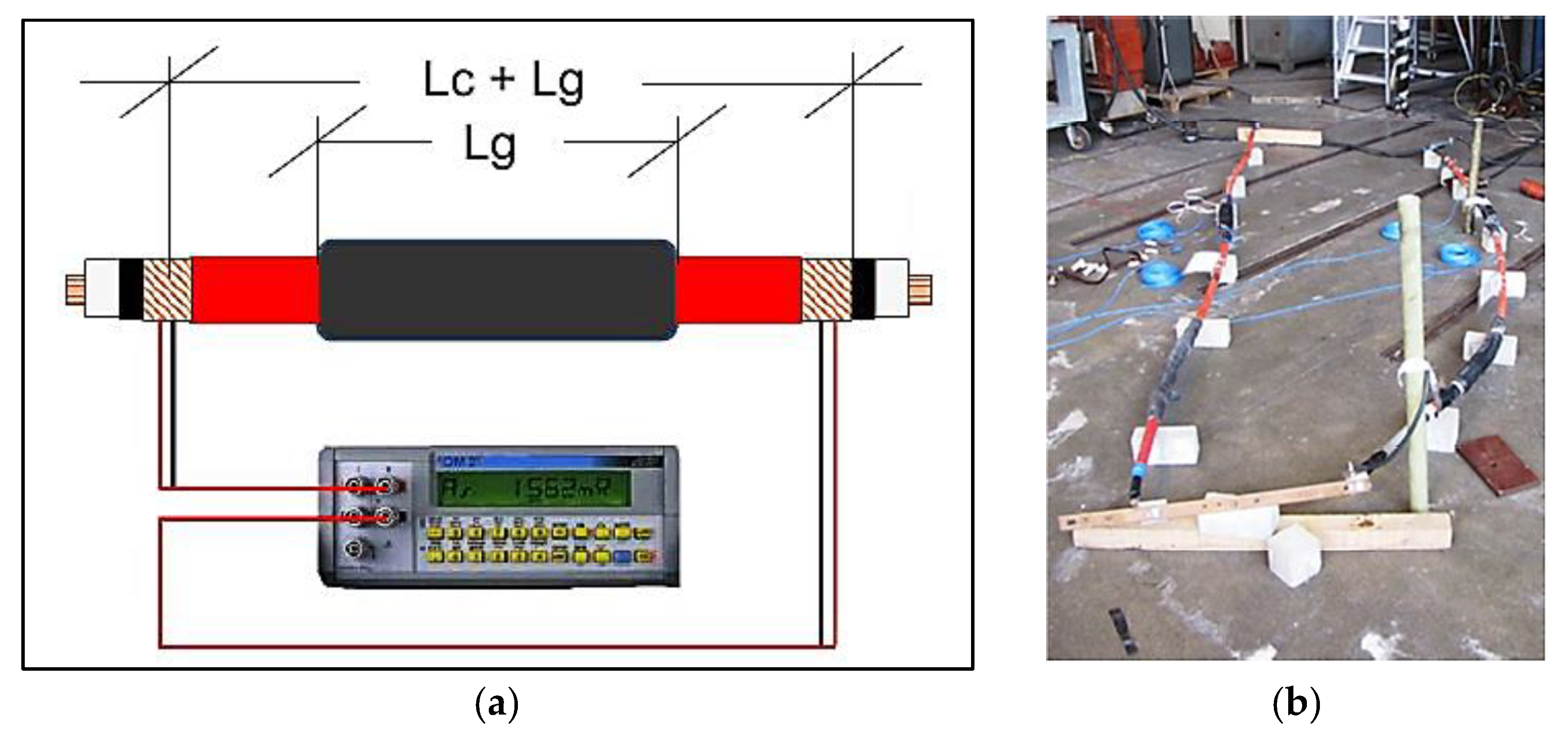
In this paper, in order to quantify the value of CR, measurements were carried out [19]. Such measurements on different joints allowed us to define a range of CR values and to take into account the different arrangements. Data were collected by a Chauvin Arnoux C.A. 6547 digital meter (Chauvin Arnoux, Paris, France), as shown in Figure 2. Results are reported in

Table 1. Measured R_s,T and CR evaluation.

Lc + Lg (m)	Lg (m)	Measured Rs,T (mΩ)	CR (mΩ)
1.08	0.75	8.693	7.743
1.03	0.75	3.11	2.225
1.03	0.75	7.076	6.191

.

In the test, both screen and joint stocking are made of copper, with 16 mm² and 100 mm² equivalent cross sections, respectively, whereas the temperature of the screen is 70 °C, leading to a 1.68 × 10⁻⁸ Ω·m resistivity value. Moreover, the distribution of the joint CR between the two joint terminals is unknown. Starting from measurements in [19], the joint CR was estimated according to the following equation:

$$CR=R_{s,T}-r_{16}\cdot \left(L_c+4\cdot L_{c,g}\right)-r_{100}\cdot L_g$$

(5)

where R_s,T is the overall screen resistance measured by the digital meter according to the configuration in Figure 2a, r₁₆ is the cable screen resistance per unit length (1.329 mΩ·m⁻¹ for the tested cable-joint system), r₁₀₀ is the joint stocking resistance per unit length (0.16 mΩ·m⁻¹ for the tested cable-joint system), L_c is the length of the portion of the cable outside the joint, L_c,g is the length over which the screen continuity is carried out (corresponding to Section 3 in Figure 1a) and L_g is the joint length, as shown in Figure 2a. Measured R_s,T values, as well as the corresponding CR values calculated with (5), are reported in Table 1.

2.2. Soil Thermal Model

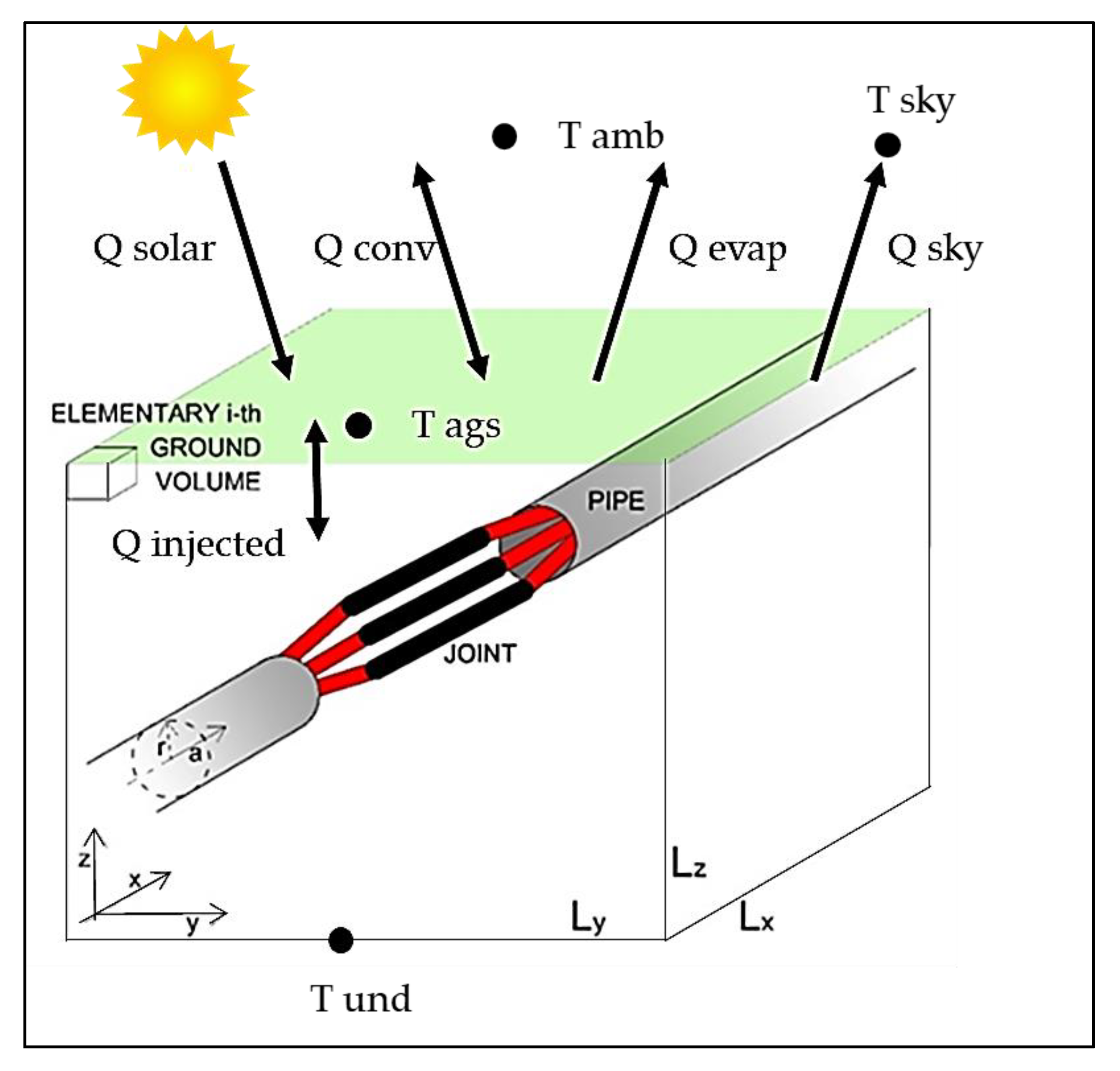
In order to represent real operating conditions (i.e., cables and joints buried in the ground), a 3D thermal model of the surrounding soil and its external surface was developed and linked to the cable-joint model described in Section 2.1. According to Figure 3, the model simulates a soil volume, in which cable and joint are buried at a certain depth; L_x, L_y, and L_z are the volume dimensions along the x, y, and z axes, respectively. The cable may be directly buried or buried in a pipe, as in Figure 3.

L_x and L_y are long enough to assume negligible thermal flows through the orthogonal surfaces; as a consequence, the heat flow at the terminals of the cable has also been neglected. The parallelepiped representing the ground has been subdivided into elementary volumes, each one simulated by resistances along the x, y, and z axes, and one capacitance directly grounded, calculated as in the following:

$$\{\begin{array}{c}{R}_{x,i}=\frac{L_x}{2n_x{\mathsf{\lambda }}_g{S}_{x,i}}\\ R_{y,i}=\frac{L_y}{2n_y{\mathsf{\lambda }}_g{S}_{y,i}}\\ R_{z,i}=\frac{L_z}{2n_z{\mathsf{\lambda }}_g{S}_{z,i}}\\ C_{g,i}=c_{g,i}\frac{L_x}{n_x}\frac{L_y}{n_y}\frac{L_z}{n_z}\end{array}$$

(6)

In Equation (6), λ_g is the thermal conductivity of the soil and c_g,i is the volumetric heat capacity of the i-th volume of soil, n_x, n_y, and n_z are the number of subdivisions, and S_x,i, S_y,i, and S_z,i are the cross sections of the i-th element along the x, y, and z axes, respectively.

The thermal conductivity was considered as varying with the temperature, according to the simplified model proposed by Ocłoń et al. in [20], by using the expression:

$${\mathsf{\lambda }}_g(T)={\mathsf{\lambda }}_{g,dry}+({\mathsf{\lambda }}_{g,wet}-{\mathsf{\lambda }}_{g,dry})\cdot \exp \left[-a_1{\left(\frac{T-T_{ref}}{a_2\cdot T_{\max ,p}}\right)}^2\right]$$

(7)

where λ_g,dry and λ_g,wet are the soil thermal conductivities in dry and wet conditions. In this paper, λ_g,dry and λ_g,wet are equal to 0.5 W∙K⁻¹∙m⁻¹ and 0.3 W∙K⁻¹∙m⁻¹, respectively. T_ref is the reference temperature, equal to 20 °C, and T_max,p is the maximum operating temperature, equal to 90 °C. Coefficients a₁ and a₂ depend on T_ref and T_max,p [20].

Regarding the surfaces orthogonal to the z-axis, the lower one was considered as isothermal at the undisturbed temperature (T_und); therefore, along z axis, resistances R_z,i are connected to an ideal independent voltage generator representing the undisturbed temperature. According to [21], T_und is the temperature of the ground layer (about 8 m deep), below which the temperature remains practically constant throughout the year. T_und has been evaluated as equal to 20 °C.

With respect to the upper surface orthogonal to z-axis, weather conditions are taken into account by means of ideal current generators that inject the heat flow Q_in, evaluated as follows [21,22]:

$$Q_{in}=Q_{solar}+Q_{conv}-Q_{sky}-Q_{evap}$$

(8)

Q_solar is the global solar radiation absorbed by this area, calculated with:

$$Q_{solar}={\mathsf{\alpha }}_{g}G$$

(9)

where α_g is the absorption heat coefficient and G represents the short-wave global solar radiation, which is calculated as follows:

$$G=\{\begin{array}{ll}0& t\le t_{rise}\\ S_{\max }\sin \left(\frac{\mathsf{\pi }(t-t_{rise})}{t_{set}-t_{rise}}\right)& t_{rise}<t<t_{set}\\ 0& t\ge t_{set}\end{array}$$

(10)

In Equation (10), t_rise and t_set are the sunrise and sunset time of the day, respectively; the peak solar irradiance S_max varies during the day and is evaluated according to [22,23] by means of the following equation:

$$S_{\max }=I_0\cdot \left(1+0.033\cdot \cos \frac{2\cdot \mathsf{\pi }\cdot d_n}{365}\right)\cdot \left(\cos L\cdot \cos \mathsf{\delta }\cdot \cos \mathsf{\omega }+\sin L\cdot \sin \mathsf{\delta }\right)$$

(11)

In Equation (11), I₀ is equal to 1000 W/m², whereas d_n is a number representing the day of a year (number one is the 1st of January), δ the declination angle evaluated according to Spencer’s equation [24], L is the Earth heliocentric latitude (in rad), and ω is the hour angle (in rad).

Q_conv is the sensible convective heat exchanged between air and the upper surface, and it depends both on soil surface temperature and on air temperature above the soil surface, T_s and T_ags, respectively, evaluated by:

$$Q_{conv}=h_{conv}\cdot (T_{ags}-T_s)$$

(12)

where h_conv is the convective heat transfer coefficient at the soil surface.

Q_sky is the heat flux due to the long-wave radiation emitted by the soil surface to the sky and is calculated as:

$$Q_{sky}=h_{rad}\cdot (T_s-T_{sky})$$

(13)

where h_rad is the thermal radiation heat exchange coefficient and T_sky the sky temperature [25].

Finally, Q_evap, which is the evaporation heat exchange flux, depends on T_ags, T_s, wind speed, ground cover, soil moisture content, and humidity; it is assessed by the equation [26,27]:

$$Q_{evap}=b_3\cdot f\cdot h_{conv}\cdot [(b_1{T}_s+b_2)-r_h\cdot (b_1{T}_{ags}+b_2)]$$

(14)

where b₁ = 103 Pa∙K⁻¹, b₂ = 609 Pa and b₃ = 0.0168 K∙Pa⁻¹; r_h is the relative humidity of the air; f is a fraction of evaporate rate, varying between 0 and 1, and depends mainly on the ground cover and moisture. For bare soil, f can be estimated as follows [22]: for saturated soil, f is equal to 1; for moist soil, f ranges from 0.6 to 0.8; for dry soil, f ranges from 0.4 to 0.5; for arid soil, f ranges from 0.1 to 0.2.

The equivalent electrical network resulting from the cable, joint, PVC pipe, and soil models is then implemented considering both the PVC pipe, where cables are located, and joint sheath as isothermal surfaces, as in [28]. The size of the network depends on the chosen discretization. In this work, the complete circuit model is composed of about 35,000 nodes. It is not possible to represent in detail the equivalent electrical network, even if an indicative section is shown, as in Figure 1.

The equivalent electrical network is solved by a home-made software developed by the authors in the Scilab environment [13,14]. The system of differential equations is solved in a transient state through the backward Euler algorithm: according to the formulation in [29], since each capacitance may be replaced by a voltage-controlled current source with a resistance in parallel, the equivalent network becomes purely resistive and is solved by nodal analysis. A more detailed description is given in [14].

3. Results

3.1. Input Data of the Simulations: Equipment and Ground Parameters, Fault Currents, and Autoreclosure Schemes

The model is applied to simulate the effect of ground faults occurring in an MV network. Fault current and fault clearing time are inputs of the problem, together with the physical and geometrical parameters of the system (i.e., cable, joint, PVC pipe, soil), which are reported in

Table 2. Inputs of the simulations (Section 1 of the joint).

Layer	Material	re (mm)	L (m)	λ (K−1·m−1·W)	c (J·K−1·m−3)
Conductor joint	Aluminium	16	0.144	237.022	2,421,630
Mastic	MNAC	21	0.144	0.2	2,000,000
Insulation	EPDM	29.1	0.144	0.2	2,000,000
Joint stocking	Copper	29.7	0.144	390.01	3,434,200
Sheath	EPDM	33.1	0.144	0.2	2,000,000

,

Table 3. Inputs of the simulations (Section 2 of the joint).

Layer	Material	re (mm)	L (m)	λ (K−1·m−1·W)	c (J·K−1·m−3)
Conductor joint	Aluminium	8.25	0.15	237.022	2,421,630
Cable insulation	HEPR	13.75	0.15	0.2	2,000,000
Mastic	MNAC	15.8	0.15	0.2	2,000,000
Insulation	EPDM	26.5	0.15	0.2	2,000,000
Joint stocking	Copper	27	0.15	390.01	3,434,200
Sheath	EPDM	30.1	0.15	0.2	2,000,000

,

Table 4. Inputs of the simulations (Section 3 of the joint).

Layer	Material	re (mm)	L (m)	λ (K−1·m−1·W)	c (J·K−1·m−3)
Conductor joint	Aluminium	8.25	0.0664	237.022	2,421,630
Cable insulation	HEPR	13.75	0.0664	0.2	2,000,000
Cable screen	Copper	14.55	0.0664	390.01	3,434,200
Cable sheath	PVC	17.75	0.0664	0.167	2,000,000
Cable screen	Copper	18.3	0.0664	390.01	3,434,200
Joint stocking	Copper	19.2	0.0664	390.01	3,434,200
Sheath	EPDM	22.6	0.0664	0.2	2,000,000

and

Table 5. Inputs of the simulations (soil parameters and coefficients).

Lx (m)	Ly (m)	Lz (m)	hconv (W·K−1·m−2)	f	αs	εs	Tund (K)	λg (W∙K−1∙m−1)	cg (J·K−1·m−3)	λg,dry (W K−1 ∙m−1)	λg,wet (W∙K1∙m−1)
2.3	4.5	10	1	0.6	0.8	0.9	293.15	0.666	1,920,000	0.3	0.5

, respectively.

Different CR values are used, corresponding to the different simulated cases, as reported in

Table 6. Contact resistance considered in the simulations.

Case	1	2	3	4	5	6
CR (mΩ)	0	0.073	0.73	1.825	3.65	7.3

. In accordance with Table 1, the maximum CR value used in the simulations is 7.3 mΩ (case 6), corresponding to about 100 times the equivalent resistance of the cable screen in Section 3 (i.e., the section in which the screen continuity in carried out); a nil CR value has also been simulated (case 1, corresponding to a perfectly installed joint). In all simulated cases, CR value has been equally shared among the two joint terminals.

As already described in Section 2.1, fault currents corresponding to CCFs were simulated, since CCFs cause very large currents (comparable to line-to-line fault currents) flowing through screens, especially if the screens are connected to the earthing system of the HV/MV substation, termed primary substation (PS) in the rest of the paper, as shown in [30,31]. The maximum simulated current value injected through screens was 10 kA, which is very uncommon in MV networks, as evidenced by the authors in [32], reporting a statistical study about fault currents due to CCFs for a typical Italian MV network, owned and managed by e-distribuzione (the most important Italian distribution system operator) and supplied by a 40 MVA transformer. In [32], the maximum calculated CCF current value is about 8.4 kA, whereas the average is about 3 kA.

Regarding fault clearing times, the reclosing cycles of circuit breakers, CBs, adopted by e-distribuzione in its MV distribution networks have been considered. Simulations have been carried out by injecting the fault current, I_F, in the core and in the screen of the MV cable. The possible presence along the MV feeder of an MV/LV substation, termed secondary substation (SS) in the rest of the paper, equipped with an automatic CB (which is a less common case in Italy, where automatic CBs are normally installed only at the beginning of the feeder), has been taken into account: in this case, different reclosing cycles have been considered, as reported in the following.

Two main UCs have been identified. The first one (named A) involves an MV feeder equipped with a CB at the beginning of the line; it is worth highlighting that this is the most common case since the protection along a MV feeder is installed only in the PS (i.e., all SSs supplied by the MV feeder are equipped with disconnectors instead of a CB). In this UC, MV feeder protection is performed by a definite-time overcurrent relay with three tripping thresholds: the first one is set at 120% of the rated ampacity, I_rated, of the MV cable (extinction time is 0.17 s if zero sequence current, I₀, is larger than 150 A, 1.07 s otherwise. Time of extinction is considered by adding the time of tripping and time of maneuver of breaker (conventionally assumed as 0.07 s); the second one is set at 800 A (extinction time is 0.17 s if I₀ is larger than 150 A, 0.32 s otherwise); the third one is set to 1400 A, with a fixed 0.12 s fault clearing time. After the extinction, reclosing cycles are performed until the fault is cleared, according to

Table 7. Autoreclosure scheme in UC A.

Current		Duration of Breaker Status (s)
IF	I0	C	O	C	O	C	O	C	UC
(1.2∙Irated, 800 A)	>150 A	0.17	0.6	0.17	30	0.17	70	0.17	A1
(1.2∙Irated, 800 A)	<150 A	1.07	0.6	1070	30	1.07	70	1.07	A2
(800 A, 1400 A)	>150 A	0.17	0.6	0.17	30	0.17	70	0.17	A1
(800 A, 1400 A)	<150 A	0.32	0.6	0.32	30	0.32	70	0.32	A2
>1400 A	-	0.12	0.6	0.12	30	0.12	70	0.12	A1

(C: CB status is “closed”; O: CB status is “open”). If the fault is not cleared after the autoreclosure cycle, a permanent opening of the CB is made (not reported in Table 7).

The second UC (named B) regards an MV feeder along which an SS is equipped with a CB (SSS in the following) with network grounded by impedance (Petersen coil); this CB defines two sections of the feeder (i.e., a section before the SSS and a section after the SSS). In such UC, the time-based overcurrent relaying coordination and the autoreclosure schemes of the circuit breaker installed in the SSS are described in

Table 8. Autoreclosure scheme in UC B, with a fault in the line section before the SSS.

Current		Duration of Breaker Status (s)
IF	I0	C	O	C	O	C	O	C	UC
>800 A	<150 A	0.32	0.6	0.32	30	0.32	70	0.32	B1

, in case the fault is located in the line section before the SSS, and

Table 9. Autoreclosure scheme in UC B, with a fault in the line section after the SSS.

Current		Duration of Breaker Status (s)
IF	I0	C	O	C	O	C	O	C	UC
(1.2∙Irated, 500 A)	>150 A	0.8	0.6	0.8	30	0.8	70	0.8	B2
>500 A1	<150 A	0.2	0.6	0.2	30	0.2	70	0.2	B2

, in case the fault is located in the line section after the SSS. In these two cases, if the fault is not cleared after the autoreclosure cycle, a permanent opening of the circuit breaker is made.

In this paper, I_rated has been assumed equal to 295 A, so that the first threshold is 354 A; moreover, thermal transients have been simulated over a 150 s timeframe in order to show the thermal behavior of the joint during a complete autoreclosure cycle.

3.2. Simulation Results

In the simulations reported in the paper, the equivalent electrical model has been applied considering a prefault cable insulation temperature equal to 90 °C, i.e., the prefault current through the MV cable was I_rated. It is worth highlighting that most results regard the section where the contact between the cable screen and the metal sheath of the joint occurs, referred to as screen continuity inside the joint, hereafter named SCJ. In addition, even if the model developed would allow, in principle, to obtain, as a result of the parametric analysis, temperatures well above those shown in the next figures (e.g., up to 5000 °C and beyond), the upper limit for temperature represented in all plots has been set to 1000 °C, as this is already far above the maximum tolerable temperature of the cable insulation during a fault (which, for the simulated cable, is 250 °C, as declared by the manufacturer).

According to Table 7, Table 8 and Table 9, the main difference between tripping thresholds is due to a SSS along the MV feeder. In order to properly compare results, UCs A1 and B1 are first considered: I_F values ranging from 1400 A and 10 kA have been injected, with a fault clearing time of 120 ms (UC A1) and 320 ms (UC B1), not simulating reclosing cycles.

Figure 4 reports the trends of maximum temperature calculated along SCJ over I_F; Figure 4a refers to UC A1, whereas Figure 4b to UC B1. According to Table 6, six different CR values are simulated for each UC (curves 1 to 6), even if case 2 is not reported since the trend is practically equal to that of case 1. Results show that if CR is nil or equal to 0.073 mΩ (case 1 and case 2 of Table 6, respectively), the 250 °C maximum allowable temperature is never exceeded in any case, whilst dangerous conditions could occur if a CR value larger than 0.73 mΩ (case 3 of Table 6) is considered. If larger CR values are considered (for instance 3.65 mΩ and 7.3 mΩ), temperatures dramatically increase and exceed the maximum allowable value also in case of common I_F values in both the UCs.

Figure 5 shows thermal transients simulated along the SCJ and the cable screen with I_F = 3 kA (the average value of I_F in [32]), using the autoreclosure scheme corresponding to UC A1 in Table 7 and considering CR values of Table 6. The whole thermal transients in SCJ for cases 1, 4, 5, and 6, as well as the thermal transient in cable screen for case 3, are reported in Figure 5a. Figure 5b shows a zoom of the same trends of Figure 5a in the timeframe of 0–2 s, in order to show the two temperature peaks corresponding to the 1st and the 2nd opening of the CB, which are not distinguishable in Figure 5a. In these cases, simulations show that SCJ does not reach dangerous temperatures if CR is lower than 3.65 mΩ, thus not impairing or breaking the joint. The trend of cable screen temperature is reported only for the simulation of case 3, since in all cases this trend is very similar to the temperature trend along the SCJ; however, it is worth noting that in case of a perfect screen contact (i.e., CR nil), the screen reaches temperatures higher than the joint because of its smaller section (not reported in other simulations). During the most severe simulated thermal transients (as in case 4, case 5, and case 6 of Figure 5), the time instant when the maximum temperature is detected corresponds to the 2nd opening of the CB: this result is consistent, since the time period between the first and the 2nd opening of the CB is very short and, consequently, temperature decreases in a negligible way.

Figure 6 shows the thermal transients in SCJ for cases 1, 2, and 3, as well as the thermal transient in cable screen for case 3, evaluated for I_F = 3 kA and using the autoreclosure scheme of UC B2 in Table 7. Simulation results show that for CR values greater than or equal to 1.825 mΩ (case 4), the maximum allowable temperature is always exceeded, thus causing the impairment or the breaking of the joint.

Figure 7 reports thermal transients evaluated with I_F = 800 A, for two different fault clearing times, namely 1070 ms and 320 ms (UC A2 in Table 7). Temperature trends are calculated for different CR values: Figure 7a reports trends for cases 1 and 3 of Table 6, whilst Figure 7b shows transients for cases 4 and 6. Thermal transients reported in Figure 7a are tolerable from the cable and joint; on the other hand, if CR = 7.3 mΩ, a fault clearing time of 1070 ms leads to unacceptable temperatures for the cable, with a maximum value equal to 310 °C.

Figure 8 reports thermal transients simulated with I_F = 1400 A, considering two different clearing times, namely 320 ms and 120 ms. Four different CR values are used: Figure 8a reports temperature trends for case 1 and case 3, whilst Figure 8b for case 4 and case 6. In this case, if CR = 7.3 mΩ, a fault clearing time of 320 ms leads to unacceptable temperatures for the cable.

In order to recap simulation results carried out according to Table 7, a correlation is further presented. Figure 9 shows the short circuit current which causes heating up to a certain limit temperature (i.e., 250 °C, 500 °C, 750 °C, and 1000 °C) as a function of CR value. Moreover, different fault clearing times have been considered; notably, 120 ms and 320 ms are reported by Figure 9a,b, respectively.

Figure 9 allows one to assess the maximum current flowing through SCJ as a function of joint CR, considering different thermal limits. With respect to the design of MV networks, this would imply that the maximum CCF current defines the maximum admissible value of the joint CR.

From Figure 9, very small differences are noticed for the two different clearing times; if different temperature limits are considered, the more the temperature limit increases, the more the offset among temperature trends decreases.

4. Discussion

Results presented in Section 3 highlight the pivotal role played by CR if large short circuit currents flow through the cable screen, as in the case of CCFs. A correct assembly of the joint does not cause appreciable CR, but if the joint is not correctly assembled (for example, joint and cable are not perfectly centered), or if the pressure applied by the shape memory sheet on both ends of the joint is reduced due to ageing, CR values up to a few milliohms may occur.

Considering circuit breaker reclosing cycles actually adopted by e-distribuzione in its MV distribution networks, practically no ground current flowing through cable screens is able to damage joints if the CR value is near 0 mΩ: in fact, for such small CR values, only ground fault currents larger than about 10 kA, tripped in 320 ms, would be able to heat the joint up to its maximum tolerable temperature, but such values are unrealistic in real MV distribution networks.

On the contrary, if the CR reaches values of some milliohms (such values have been measured in healthy joints in operation, as reported in [19]), realistic ground fault current values are able to damage and/or to break the joint, depending on fault clearing time and CR value. Parametric analyses, as reported in Figure 4 and Figure 9, show that for CR values of about 2 mΩ, I_F values of about 4 kA are detrimental even for fast fault clearing times (120 ms); with larger CR values (about 6–7 mΩ), CCFs practically always cause an unacceptable heating of the joint.

5. Conclusions

The paper presents a study focused on the thermal stress on MV cables and their joints due to ground fault currents flowing through cable screens. A complete 3D thermal model (including a cable line buried into the ground, the attendant joints and the surrounding soil), already developed by the authors and validated through experimental tests, has been used. In this paper, the model was extended in order to take into account the effect of joint contact resistance, due to either an inaccurate joint manufacturing or grip slackening during operation.

Ground fault currents caused by cross country faults, whose values are comparable to line-to-line fault currents, were injected into the model; in addition, in order to represent real operating conditions for cable and joint during faults, autoreclosure schemes normally adopted by Italian DSOs in MV distribution networks were simulated.

A parametric study including a massive number of thermal transients and considering different autoreclosure schemes as well as different ground current and joint contact resistance values, shows that the latter plays a key role on joint and cable heating. For contact resistance values near zero, practically no ground current is able to damage the joint, whereas if resistances larger than few milliohms are taken into account, the maximum tolerable temperature of cable and joint insulation is exceeded also for common values of CCF currents and very fast fault clearing times.

In order to reduce joint failures, it is necessary, on one hand, to study solutions able to reduce the currents flowing in the shields during ground failures (thus minimizing thermal stresses at the points of continuity between the cable screen and the copper stocking), and, on the other hand, to avoid errors in the joint manufacturing which can introduce high contact resistances (able to produce hotspots during the circulation of ground fault currents).

In subsequent work, the authors will analyze in detail some possible solutions to mitigate thermal stresses in the joints due to currents flowing in the screens.

References

1. Unareti. Piano di Interventi per l’Incremento della Resilienza della Rete Elettrica di Distribuzione di Unareti. 2019. Available online: https://www.unareti.it/unr/unareti/Piano-di-lavoro-per-incremento-resilienza-2019-2021.pdf (accessed on 7 August 2019).
2. Bosisio, A.; Berizzi, A.; Bovo, C.; Amaldi, E.; Fratti, S. GIS-based Urban Distribution Networks Planning with 2-step Ladder Topology Considering Electric Power Cable Joints. In Proceedings of the 2018 110th AEIT International Annual Conference, Bari, Italy, 3–5 October 2018. [Google Scholar] [CrossRef]
3. Jongen, R.A.; Morshuis, P.H.F.; Smith, J.J.; Janssen, A.L.J. Influence of Ambient Temperature on the Failure Behavior of Cable Joints. In Proceedings of the 2007 Annual Report—Conference on Electrical Insulation and Dielectric Phenomena (CEIDP), Vancouver, BC, Canada, 14–19 October 2007; pp. 643–646. [Google Scholar] [CrossRef]
4. Aziz, M.M.A.; Riege, H. A new method for cable joints thermal analysis. IEEE Trans. Power Appl. Syst. 1980, 99, 2386–2391. [Google Scholar] [CrossRef]
5. Zhang, L.; LuoYang, X.; Le, Y.; Yang, F.; Gan, C.; Zhang, Y. A thermal probability density–based method to detect the internal defects of power cable joints. Energies 2018, 11, 1674. [Google Scholar] [CrossRef]
6. Ruan, J.; Zhan, Q.; Tang, L.; Thang, K. Real-time temperature estimation of three-core medium-voltage cable joint based on support vector regression. Energies 2018, 11, 1405. [Google Scholar] [CrossRef]
7. Tang, L.; Ruan, J.; Qiu, Z.; Liu, C.; Tang, K. Strongly robust approach for temperature monitoring of power cable joint. IET Gener. Transm. Distrib. 2019, 13, 1324–1331. [Google Scholar] [CrossRef]
8. Yang, F.; Cheng, P.; Luo, H.; Yang, Y.; Liu, H.; Kang, K. 3-D thermal analysis and contact resistance evaluation of power cable joint. Appl. Therm. Eng. 2016, 93, 1183–1192. [Google Scholar] [CrossRef]
9. Jin, F.; Peng, C.; Wei, C.; Hu, X.; Qian, W.; Qi, Y.; Fan, Y. Investigation of the effects of insulation defects on the 3-D electromagnetic-thermal coupling fields of power cable joint. In Proceedings of the 2016 11th AEIT International Conference on Industrial Electronics and Application (ICIEA), Hefei, China, 5–7 June 2016. [Google Scholar] [CrossRef]
10. Yang, F.; Liu, K.; Cheng, P.; Wang, S.; Wang, X.; Gao, B.; Fang, Y.; Xia, R.; Ullah, I. The coupling fields characteristics of cable joints and application in the evaluation of crimping process defects. Energies 2016, 9, 932. [Google Scholar] [CrossRef]
11. Wang, P.; Liu, G.; Ma, H.; Liu, Y.; Xu, T. Investigation of the ampacity of a prefabricated straight-through joint of high voltage cable. Energies 2017, 10, 2050. [Google Scholar] [CrossRef]
12. Yang, F.; Zhu, N.; Liu, G.; Ma, H.; Wei, X.; Hu, C.; Wang, Z.; Huang, J. A new method for determining the connection resistance of the compression connector in cable joint. Energies 2018, 11, 1667. [Google Scholar] [CrossRef]
13. Bragatto, T.; Cresta, M.; Gatta, F.M.; Geri, A.; Maccioni, M.; Paulucci, M. Underground MV power cable joints: A nonlinear thermal circuit and its experimental validation. Electr. Power Syst. Res. 2017, 149, 190–197. [Google Scholar] [CrossRef]
14. Bragatto, T.; Cresta, M.; Gatta, F.M.; Geri, A.; Maccioni, M.; Paulucci, M. A 3-D nonlinear thermal circuit model of underground MV power cables and their joints. Electr. Power Syst. Res. 2019, 173, 112–121. [Google Scholar] [CrossRef]
15. Anders, G.J. Rating of Electric Power Cables: Ampacity Computations for Transmission, Distribution, and Industrial Applications; McGraw Hill Publishing Co.: New York, NY, USA, 1997; ISBN 0070017913. [Google Scholar]
16. Greenwood, J.A. Constriction resistance and the real area of contact. Br. J. Appl. Phys. 1966, 17, 1621–1632. [Google Scholar] [CrossRef]
17. Boyer, L. Contact resistance calculations: Generalizations of Greenwood’s formula including interface films. Trans. Compon. Packag. Technol. 2001, 24, 50–58. [Google Scholar] [CrossRef]
18. Vogler, M.; Sheppard, S. Electric contact resistance under high loads and elevated temperatures. Weld. J. Incl. Weld. Res. Suppl. 1993, 72, 231–238. [Google Scholar]
19. CESI. Prove di Diagnostica su Giunti di Cavo mt—Prove di cortocircuito di giunti di cavi MT e servizio di Analisi; Technical Report for E-Distribuzione; CESI: Milan, Italy, 2017. [Google Scholar]
20. Ocłoń, P.; Cisek, P.; Pilarczyk, M.; Taler, D. Numerical simulation of heat dissipation processes in underground power cable system situated in thermal backfill and buried in a multilayered soil. Energy Convers. Manag. 2015, 95, 352–370. [Google Scholar] [CrossRef]
21. Ouzzane, M.; Eslami-Nejad, P.; Badache, M.; Aidoun, Z. New correlations for the prediction of the undisturbed ground temperature. Geothermics 2015, 53, 379–384. [Google Scholar] [CrossRef]
22. Badache, M.; Eslami-Nejad, P.; Ouzzane, M.; Aidoun, Z.; Lamarche, L. A new modeling approach for improved ground temperature profile determination. Renew. Energy 2016, 85, 436–444. [Google Scholar] [CrossRef]
23. Sung, T.; Yoon, S.Y.; Kim, K.C. A mathematical model of hourly solar radiation in varying weather conditions for a dynamic simulation of the solar organic rankine cycle. Energies 2015, 8, 7058–7069. [Google Scholar] [CrossRef]
24. Spencer, J. Fourier series representation of the position of the sun. Search 1971, 2, 162–172. [Google Scholar]
25. Berdahl, P.; Fromberg, R. The thermal radiance of clear skies. Sol. Energy 1982, 29, 299–314. [Google Scholar] [CrossRef]
26. Krarti, M.; Lopez-Alonzo, C.; Claridge, D.E.; Freider, J.F. Analytical model to predict annual soil surface temperature variation. J. Sol. Energy Eng. 1995, 117, 91–99. [Google Scholar] [CrossRef]
27. Mihalakakou, G. On estimating soil surface temperature profiles. Energy Build. 2002, 34, 251–259. [Google Scholar] [CrossRef]
28. De Lieto Vollaro, R.; Fontana, L.; Vallati, A. Thermal analysis of underground electrical power cables buried in non-homogeneous soils. Appl. Therm. Eng. 2011, 31, 772–778. [Google Scholar] [CrossRef]
29. Chua, L.; Lin, P.M. Computer-Aided Analysis of Electronic Circuits: Algorithms and Computational Techniques; Prentice Hall: Upper Saddle River, NJ, USA, 1975; ISBN 0131654152. [Google Scholar]
30. Gatta, F.M.; Geri, A.; Lauria, S.; Maccioni, M. An equivalent circuit for the evaluation of cross-country fault currents in medium voltage (MV) distribution networks. Energies 2018, 11, 1929. [Google Scholar] [CrossRef]
31. Benato, R.; Sessa, S.D.; Rinzo, G.; Marchese, O.; Tanzi, L.; Zapelloni, R. Different Screen Arrangements of Distribution Insulated Cables. In Proceedings of the 2018 110th AEIT International Annual Conference, Bari, Italy, 3–5 October 2018. [Google Scholar] [CrossRef]
32. Gatta, F.M.; Geri, A. Studi di Rete Finalizzati all’Analisi ed alla Predizione delle Correnti di Corto Circuito e dei loro Effetti negli Schermi dei Cavi delle Reti di Distribuzione in MT a Seguito di Guasti Monofase o Polifase, Singoli o Multipli Tenendo in Considerazione le Due Possibili Alternative di Schermi Connessi in un Unico Nodo (Cabina Primaria e/o Centro Satellite) o di Schermi Interrotti; Technical Report for E-Distribuzione; Internal report; Rome, Italy, 2018. (In Italian) [Google Scholar]
Figure 1. (a) Simulated cold-shrinkable joint (the cylindrical coordinate system used in the model is also shown), extracted from [14]; (b) Equivalent electrical circuit corresponding to each layer of the cable; (c) Detail of the equivalent network representing the contact resistance (CR).
Energies 12 03496 g001
Figure 2. (a) Outline of the experimental setup for CR measurements; (b) Laboratory setup for the tests [19].
Energies 12 03496 g002
Figure 3. The complete simulated system.
Energies 12 03496 g003
Figure 4. Maximum temperature calculated for short circuit currents cleared in 120 ms (a) and 320 ms (b); different CR values are simulated, as defined in Table 6.
Energies 12 03496 g004
Figure 5. (a) Thermal transients in SCJ (cases 1, 4, 5, and 6) and in the cable screen (case 3). IF = 3 kA, UC A1. (b) Zoom of (a) in the timeframe from 0 s to 2 s.
Energies 12 03496 g005
Figure 6. Thermal transients for IF = 3 kA (UC B2). (a) Cases 1, 2, and 3; (b) Cases 4, 5, and 6.
Energies 12 03496 g006
Figure 7. Thermal transients along SCJ, IF = 800 A; fault clearing times: 1070 ms (solid line) and 320 ms (dashed line). (a) Cases 1 and 3; (b) Cases 4 and 6.
Energies 12 03496 g007
Figure 8. Thermal transients along SCJ, IF = 1400 A; fault clearing times: 320 ms (solid line) and 120 ms (dashed line). (a) Cases 1 and 3; (b) Cases 4 and 6.
Energies 12 03496 g008
Figure 9. Fault current values causing SCJ heating up to the maximum tolerable temperature, as a function of joint CR. Four different maximum tolerable temperature are considered: 250 °C (solid line), 500 °C (dotted line), 750 °C (short-dashed line), and 1000 °C (long-dashed line). (a) 120 ms fault clearing time (UC A1); (b) 320 ms fault clearing time (UC B1).
Energies 12 03496 g009