Application of a Deep Deterministic Policy Gradient Algorithm for Energy-Aimed Timetable Rescheduling Problem

Abstract

Reinforcement learning has potential in the area of intelligent transportation due to its generality and real-time feature. The Q-learning algorithm, which is an early proposed algorithm, has its own merits to solve the train timetable rescheduling (TTR) problem. However, it has shortage in two aspects: Dimensional limits of action and a slow convergence rate. In this paper, a deep deterministic policy gradient (DDPG) algorithm is applied to solve the energy-aimed train timetable rescheduling (ETTR) problem. This algorithm belongs to reinforcement learning, which fulfills real-time requirements of the ETTR problem, and has adaptability on random disturbances. Superior to the Q-learning, DDPG has a continuous state space and action space. After enough training, the learning agent based on DDPG takes proper action by adjusting the cruising speed and the dwelling time continuously for each train in a metro network when random disturbances happen. Although training needs an iteration for thousands of episodes, the policy decision during each testing episode takes a very short time. Models for the metro network, based on a real case of the Shanghai Metro Line 1, are established as a training and testing environment. To validate the energy-saving effect and the real-time feature of the proposed algorithm, four experiments are designed and conducted. Compared with the no action strategy, results show that the proposed algorithm has real-time performance, and saves a significant percentage of energy under random disturbances.

1. Introduction

Nowadays, artificial intelligence (AI) has successfully been used for understanding human speech [1,2], competing at a high level in strategic game systems (such as Chess [3] and Go [4,5]), self-driving vehicles [6,7], and interpreting complex data [8,9]. Reinforcement learning (RL) [10,11], which is a vital branch of AI, has potential in the area of intelligent transportation. There are two advantages of RL: First, due to its generality, agents can effectively study many disciplines in a complex environment such as the metro network [12,13,14]; second, an agent with full exploration of the environment can give proper decisions in real-time, which means that RL can be used in optimization problems with real-time requirements. Until now, the train timetable rescheduling (TTR) problem [15,16,17,18] has been repeatedly discussed, however, there is only a small amount of literature using RL as a possible solution. Šemrov et al. [19] used a rescheduling method based on RL in a railway network in Slovenia. They illustrated that the rescheduling effect of the proposed method were at least equivalent and often superior to the simple first-in-first-out (FIFO) method and the random walk method. Yin et al. [20] developed an intelligent train operation (ITO) algorithm based on RL to calculate optimal decisions, which minimize the reward for both total time-delay and energy-consumption. Both literatures are based on the Q-learning algorithm [21,22] belonging to RL. However, Q-learning is limited by the dimensionality of action: The number of action increases exponentially with the number of degrees of freedom [23].

The energy-aimed train timetable rescheduling (ETTR) problem is rarely mentioned in previous literatures. It is different from traditional TTR problems, which focus on minimizing the total delay time of passengers [18] or minimizing the overall delays of all trains [24,25], the ETTR problem focuses on the energy optimization after disturbances break the pre-scheduled timetable. Gong et al. [26] proposed an integrated energy-efficient operation methodology (EOM) to solve the ETTR problem. The objectives are compensating dwell time disturbances in real-time and reducing the total energy in a whole travel. EOM saves the overall energy consumption by reducing the travel time in the next sections immediately after a delay and pulling the delayed train back to the original optimal timetable, although temporarily more energy is consumed in the transition process.

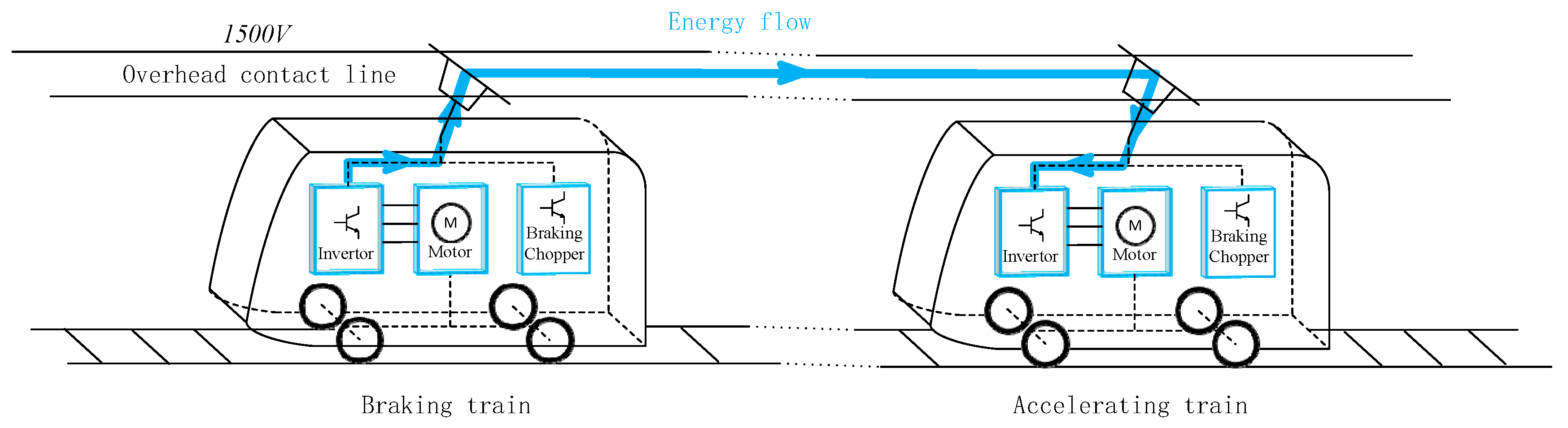
In this paper, DDPG is applied to solve the ETTR problem. This algorithm is a model-free, off-policy actor-critic algorithm using deep function approximators that can learn policies in high-dimensional, continuous action spaces [23]. It is successfully applied in fields such as robotic control [27] and traffic light timing optimization [28]. Superior to Q-learning, both state spaces and action spaces are continuous [29], which means that the observation values such as the speed and position of trains are continuous, and the target values such as the rescheduled travel time and dwelling time are also continuous. EOM only reschedules the delayed train, however, DDPG reschedules all trains in the network immediately after a disturbance happens.

The remainder of the paper is organized as follows. Section 2 introduces the principles of DDPG for a regular system. Section 3 presents three models for the metro network: Train traffic model, train movement model, and energy consumption model. In Section 4, four experiments based on a real-world network of the Shanghai Metro Line 1 (SML1) is presented to validate the DDPG algorithm. The final section concludes the paper.

2. Principles of Deep Deterministic Policy Gradient

DDPG, a recently developed algorithm in reinforcement learning, is used to solve complex tasks from an unprocessed, high-dimensional, sensory input [23]. This algorithm is comparable to the human level in many Atari video games. However, it has not been used in the area of intelligent transportation. This algorithm inherits its own advantage from earlier algorithms such as Q-learning and the deep Q-network [30]. What is more, compared with Q-learning, it has continuous action space. Compared with the deep Q-network, it has a policy network to provide deterministic action. In the following, the principle of DDPG is introduced.

Obeying a standard reinforcement learning setup, an agent interacts with an environment in discrete timesteps based on a Markov decision process (MDP). At each timestep $t$, the agent receives state $s_t$, takes action $a_t$, and receives reward $r_t$. At the next timestep, the environment receives the action $a_t$ and generates new state $s_{t+1}$ with transition dynamics $p\left(s_{t+1}|s_t,a_t\right)$. The state space is $\mathrm{S}$ and the action space is $\mathrm{A}={ℝ}^N$. Previous RL algorithms such as the deep Q-network define the target policy $\pi :\mathrm{S}\to \mathrm{P}\left(\mathrm{A}\right)$, which maps the state to a probability distribution over the action. The action–value function describes an expected return after taking action $a_t$ in state $s_t$ and thereafter following policy $\mathsf{\pi }$, which is formulated according to the Bellman equation:

$$Q^{\mathsf{\pi }}\left(s_t,a_t\right)={\mathbb{E}}_{r_t,s_{t+1}\sim E}\left[r\left(s_t,a_t\right)+\gamma {\mathbb{E}}_{a_{t+1}\sim \mathsf{\pi }}\left[Q^{\mathsf{\pi }}\left(s_{t+1},a_{t+1}\right)\right]\right]$$

(1)

where the discounting factor meets $\gamma \in \left[0,1\right]$.

Both DDPG and Q-learning have a deterministic policy gradient. The deterministic policy gradient is the expected gradient of the action–value function gradient, which can be estimated much more efficiently than the usual stochastic policy gradient [29]. Considering the target policy $\mu :\mathrm{S}\to \mathrm{A}$ directly maps state to deterministic action, the action–value function is formulated as:

$$Q^{\mu }\left(s_t,a_t\right)={\mathbb{E}}_{r_t,s_{t+1}\sim E}\left[r\left(s_t,a_t\right)+\gamma Q^{\mu }\left(s_{t+1},\mu \left(s_{t+1}\right)\right)\right]$$

(2)

where $Q^{\mu }$ can be learned off-policy.

Q-learning [21] uses the greedy policy $\mu \left(s\right)=\arg {\max }_{a}Q\left(s,a\right)$ to update the action–value function, then the training iteration of $Q^{\mu }$ is formulated as:

$$Q^{\mu }\left(s_t,a_t\right)\leftarrow Q^{\mu }\left(s_t,a_t\right)+\alpha \left[r\left(s_t,a_t\right)+\gamma \underset{a_{t+1}}{\max }{Q}^{\mu }\left(s_{t+1},a_{t+1}\right)-Q^{\mu }\left(s_t,a_t\right)\right]$$

(3)

where $\alpha$ is the learning rate. $Q^{\mu }$ in Q-learning is a table, which provides a limit space for possible values of action and state, so Q-learning cannot be straightforwardly used in a continuous space.

DDPG is a member of the actor-critic algorithm, which contains four neural networks: Current critic network $Q\left(s,a|{\theta }^Q\right)$, current actor network $\mu \left(s|{\theta }^{\mu }\right)$, target critic network $Q^{\prime }\left(s,a|{\theta }^{Q^{\prime }}\right)$ and target actor network ${\mu }^{\prime }\left(s|{\theta }^{{\mu }^{\prime }}\right)$, where ${\theta }^Q$, ${\theta }^{\mu }$, ${\theta }^{Q^{\prime }}$ and ${\theta }^{{\mu }^{\prime }}$ are the weights of each network. $Q^{\prime }$ and ${\mu }^{\prime }$ are a copy of $Q$ and $\mu$ respectively in the structures. Both ${\theta }^{Q^{\prime }}$ and ${\theta }^{{\mu }^{\prime }}$ are partially updated from the current networks at each timestep. The current critic network is updated by minimizing the loss function:

$$L\left({\theta }^Q\right)={\mathbb{E}}_{{\mu }^{\prime }}\left[{\left(y_t-Q\left(s_t,a_t|{\theta }^Q\right)\right)}^2\right]$$

(4)

where

$$y_t=r\left(s_t,a_t\right)+\gamma Q^{\prime }\left(s_{t+1},{\mu }^{\prime }\left(s_{t+1}|{\theta }^{{\mu }^{\prime }}\right)|{\theta }^{Q^{\prime }}\right)$$

(5)

The current actor network is updated by the gradient function:

$${\nabla }_{{\theta }^{\mu }}\mu \approx {\mathbb{E}}_{{\mu }^{\prime }}\left[{\nabla }_{a}Q\left(s,a|{\theta }^Q\right)|{}_{s=s_t,a=\mu \left(s_t\right)}{\nabla }_{{\theta }^{\mu }}\mu \left(s|{\theta }^{\mu }\right)|{}_{s=s_t}\right]$$

(6)

The gradient function is continuous, which ensures that the action of the agent is updated within a continuous space. The specific Algorithm 1 process is described as follows:

Algorithm 1. DDPG algorithm

Randomly initialize critic network $Q\left(s,a|{\theta }^Q\right)$, actor network $\mu \left(s|{\theta }^{\mu }\right)$ with weights ${\theta }^Q$ and ${\theta }^{\mu }$.

Initialize target network $Q^{\prime }$ and ${\mu }^{\prime }$ with weights ${\theta }^{Q^{\prime }}\leftarrow {\theta }^Q,{\theta }^{{\mu }^{\prime }}\leftarrow {\theta }^{\mu }$

Initialize replay buffer $R$

for $episode=1$ to $M$ do

Initialize a random process $N$

Receive initial state $s_1$ from environment $E$

for $t=1$ to $T$ do

Select action $a_t=\mu \left(s_t|{\theta }^{\mu }\right)+N_t$ according to the current actor network

Execute action $a_t$ in the environment $E$ , and receive reward $r_t$ and new state $s_{t+1}$

Store transition $\left(s_t,a_t,r_t,s_{t+1}\right)$ in buffer $R$

Sample a random minibatch of $N$ transitions $\left(s_i,a_i,r_i,s_{i+1}\right)$ from $R$

Set $y_i=r_i+\gamma Q^{\prime }\left(s_{i+1},{\mu }^{\prime }\left(s_{i+1}|{\theta }^{{\mu }^{\prime }}\right)|{\theta }^{Q^{\prime }}\right)$

Update the critic by minimizing the loss: $L=\frac{1}{N}{{\displaystyle {\sum }_i\left[y_i-Q\left(s_i,a_i|{\theta }^Q\right)\right]}}^2$

Update the actor policy using the sampled gradient:

${\nabla }_{{\theta }^{\mu }}\mu |{}_{s_i}\approx \frac{1}{N}{\displaystyle {\sum }_i{\nabla }_{a}Q\left(s,a|{\theta }^Q\right)|{}_{s=s_i,a=\mu \left(s_i\right)}{\nabla }_{{\theta }^{\mu }}\mu \left(s|{\theta }^{\mu }\right)|{}_{s=s_i}}$

Update the target networks:

${\theta }^{Q^{\prime }}\leftarrow \tau {\theta }^Q+\left(1-\tau \right){\theta }^{Q^{\prime }},{\theta }^{{\mu }^{\prime }}\leftarrow \tau {\theta }^{\mu }+\left(1-\tau \right){\theta }^{{\mu }^{\prime }}$

end for

end for

3. Models for Metro Network

In order to describe the operational process in a metro network, three models are formulated: A model of the train traffic, a model of the energy consumption, and a model of the train movement.

3.1. Model of Train Traffic

The model of train traffic defines the departure and arrival instant for each train in a metro network. The departure instant of the No. m train at the starting station is defined as:

$$t_{de}^{m,1}=\left(m-1\right)t_h$$

(7)

where $t_h$ is the headway. The departure instant of the No. m train at the No. n station is defined as:

$$t_{de}^{m,n}=t_{de}^{m,1}+{\displaystyle \sum _{i=1}^{n-1}\left(t_t^{m,i}+t_{dw}^{m,i+1}\right)}$$

(8)

where $t_t^{m,i}$ represents the travel time of the No. m train from the No. i station to the No. i+1 station, and $t_{dw}^{m,i+1}$ represents the dwelling time of the train at the No. i+1 station.

If a disturbance $\epsilon$ happens at the No. n station, the dwell time will be $t_{dw}^{m,n}+\epsilon$, then the departure instant of the No. m train at the No. n station is defined as:

$$t_{de}^{m,n}=t_{de}^{m,1}+{\displaystyle \sum _{i=1}^{n-1}\left(t_t^{m,i}+t_{dw}^{m,i+1}\right)}+\epsilon$$

(9)

To simplify the ETTR problem, we assume that only one disturbance happens during a complete test procedure from the first train’s departure to the last train’s arrival. The instant of the last train arriving to the terminal station is defined as

$$t_a^{M,N}=t_{de}^{M,1}+{\displaystyle \sum _{i=1}^{N-2}\left(t_t^{M,i}+t_{dw}^{M,i+1}\right)}+t_t^{M,N-1}+\epsilon$$

(10)

where $M$ is the total train number and $N$ is the total station number, $t_a^{M,N}$ also represents the total time for the simulation.

3.2. Model of Energy Consumption

The train regulation directly affects the energy consumption of metro networks. Considering a metro network with several trains driving in different strategies, traction trains consume energy while braking trains recover energy at the same time. If trains are regulated in a proper way, a large amount of energy can be saved. Figure 1 shows the energy flow between trains.

The net value of the energy consumption in each test is defined as:

$$E=E_T-E_R={\displaystyle {\int }_0^{t_a^{M,N}}{P}_T}dt-{\displaystyle {\int }_0^{t_a^{M,N}}{P}_R}dt$$

(11)

where $E_T$ is the traction energy, $E_R$ is the recovery energy, $P_T$ is the traction power, and $P_R$ is the recovery power. $P_T$ is defined as

$$P_T=\frac{{\displaystyle \sum _{m=1}^{M}T\left(v^m\right)v^m}}{{\beta }_1}$$

(12)

where $T\left(v^m\right)$ is the traction force of the No. m train in the acceleration phase and the cruising phase, $v^m$ is the driving speed, and ${\beta }_1$ is the conversion efficiency from electricity to mechanical energy.

$P_R$ is the minimum value between the traction power and braking power. If the traction power is larger than the braking power, the braking power will be fully utilized; otherwise the heating resistors will consume the extra braking power. Accordingly, $P_R$ is defined as:

$$P_R=\min \left(P_T,{\beta }_3{P}_B\right)$$

(13)

where ${\beta }_3$ is the recovery coefficient on the braking energy, and $P_B$ is defined in a formulation as follows:

$$P_B={\displaystyle \sum _{m=1}^{M}B\left(v^m\right)v^m}{\beta }_2$$

(14)

where ${\beta }_2$ is the conversion efficiency from mechanical energy to electrical energy, and $B\left(v^m\right)$ is the braking force of the No. m train in the braking phase.

3.3. Model of Train Movement

The optimal control strategy of a metro train is in a sequence of maximum acceleration, cruising, and maximum braking [31].

In the acceleration phase, $B\left(v^m\right)=0$, and $T\left(v^m\right)$ meets the characteristic curves [32,33,34] in Figure 2, where $\left(p_1,q_1,p_2\right)$ are parameters and $v_1$ is the constant.

In the cruising phase, $B\left(v^m\right)=0$, and $T\left(v^m\right)=r\left(v^m\right)-g\left(x^m\right)$, where $g\left(x^m\right)$ represents the gravity relating to the gradient of track, and $r\left(v^m\right)$ meets Davis’s Equation [35]

$$r\left(v^m\right)={\lambda }_1{\left(v^m\right)}^2+{\lambda }_2{v}^m+{\lambda }_3$$

(15)

where ${\lambda }_1$, ${\lambda }_2$ and ${\lambda }_3$ are parameters.

In the braking phase, $T\left(v^m\right)=0$, and $B\left(v^m\right)$ are shown in Figure 3, where $\left(p_3,q_2,p_4\right)$ are parameters and $v_2$ is the constant.

3.4. Relation among Three Models

Numerical examples are based on the data of the Shanghai Metro Line 1, a network with narrow spacing between adjacent stations [26]. Hence, trains travel in each section in a sequence of accelerating-cruising-braking, without repeated accelerating and braking. The cruising speed $v_c^{m,n}$ has a one-to-one mapping from the travel time in interstation $t_t^{m,n}$. As shown in Figure 4, the area enclosed by the red curve and axis $t$ indicates the section spacing. If the cruising speed increases to $v_c^{m,n}{}^{\prime }$, the travel time will decrease to $t_t^{m,n}{}^{\prime }$ to keep the section spacing constant, as the blue curve shows.

4. Apply DDPG to ETTR

The ETTR problem is regarded as a complex problem for the reason of three points. First, it is a typical non-convex optimization problem. There are many local minimum points leading to difficultly searching the optimal schedule. Second, this problem has a high-quality real-time requirement. Disturbances in a metro network will bring a series of chain reactions that make an offline schedule not optimal anymore. Third, disturbances occur randomly at different stations on different trains, and the length of the disturbances is stochastic.

In this section, DDPG, a model-free, off-policy actor-critic algorithm, is proposed to solve the ETTR problem. The algorithm is able to solve the three points above properly. First, the proposed method has an advantage in solving complex non-convex optimization problems. Second, it reschedules the timetable in real-time, which effectively avoids chain reactions and saves more energy. Third, it has self-adaptability to make appropriate choices according to disturbances. According to the introduction of the DDPG algorithm in Section 2, neural networks take an important role, which correct themselves during each training episode, and provide good advices for an agent during each testing episode. The well-trained neural networks can deduce the result in real-time during each policy decision process.

The environment and its state, agent and its action, and the reward feedback are the five fundamental components of DDPG. In the following, the definition details are provided to solve the specific ETTR problem.

4.1. Environment and Agent

To solve the ETTR problem, an environment is established in Section 3. A single agent is introduced, which makes proper decisions when disturbances happen. Different from playing video games, the agent does not need to take action at each timestep, but rather, make decisions in the departure instant of each train. Disturbances always happen in the dwelling time, caused by a sudden peak point of passenger flow. Hence, the agent needs to adjust the travel time and dwelling time after the disturbances, and take advantage of the recover energy as much as possible.

4.2. State

The state selection is an important step of the DDPG algorithm, which directly affects the accuracy of decisions made by the agent. Increasing the dimension of state spaces will increase the complexity of the actor network, leading to a more training period. However, the more complex network structure helps the agent to have a deeper understanding to the environment. In the ETTR problem based on the two-train network, five quantities are chosen for the observation of the agent: The number of the departing train and its last dwelling time, the control strategy, and the current speed/position of the other running trains. In the three-train network, the dimension of the state space will be eight. Normalization is needed in the state inputs.

4.3. Action

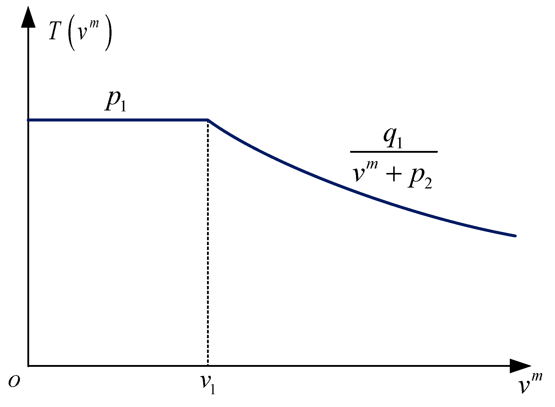
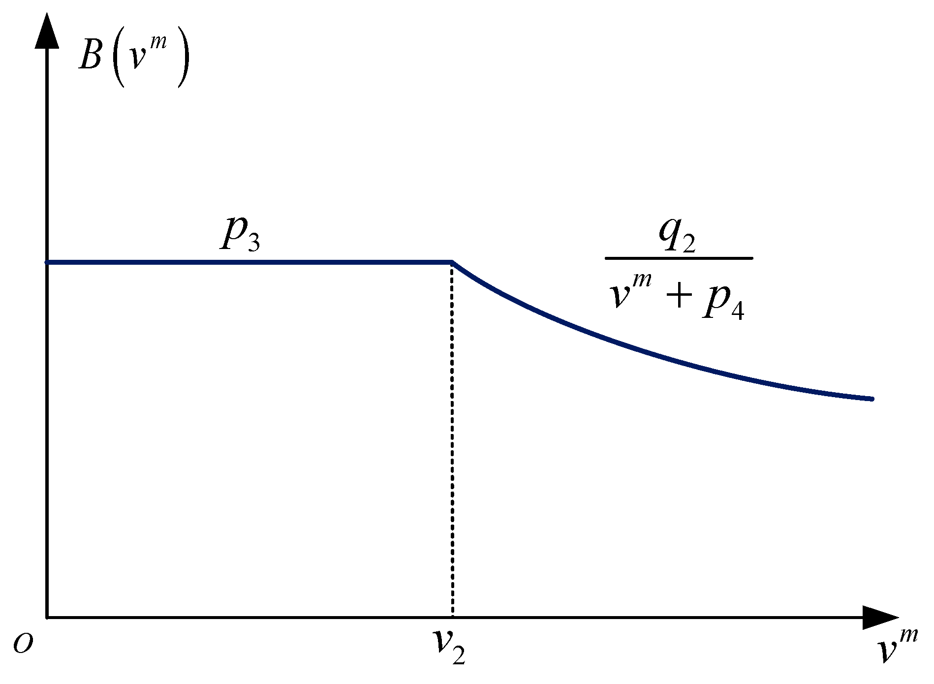
The objective of the agent is to find a proper travel time and dwelling time for the departing train. In Section 3.4, the relation between the travel time and the cruising speed is formulated. Hence, it is reasonable to define the action as the cruising speed and the dwelling time of the departing train. Both actions have upper bounds and lower bounds.

4.4. Rewards

Disturbances happen randomly at different stations on different trains. The duration of each disturbance has random values. Rewards of the agent are set to maximize the recover energy and minimize the traction energy of the DDPG. Weight coefficients are essential, which make sure that the recover energy and the traction energy are in the same order of magnitude. The reward function is formulated as follows.

$$r_t=\{\begin{array}{cc}0& 0\le t<t_a^{M,N}\\ \left[\left(E_{R_{DDPG}}-E_{R_{No-action}}\right)\ast 0.9+\left(E_{T_{No-action}}-E_{T_{DDPG}}\right)\ast 0.1\right]/\lambda & t=t_a^{M,N}\end{array}$$

(16)

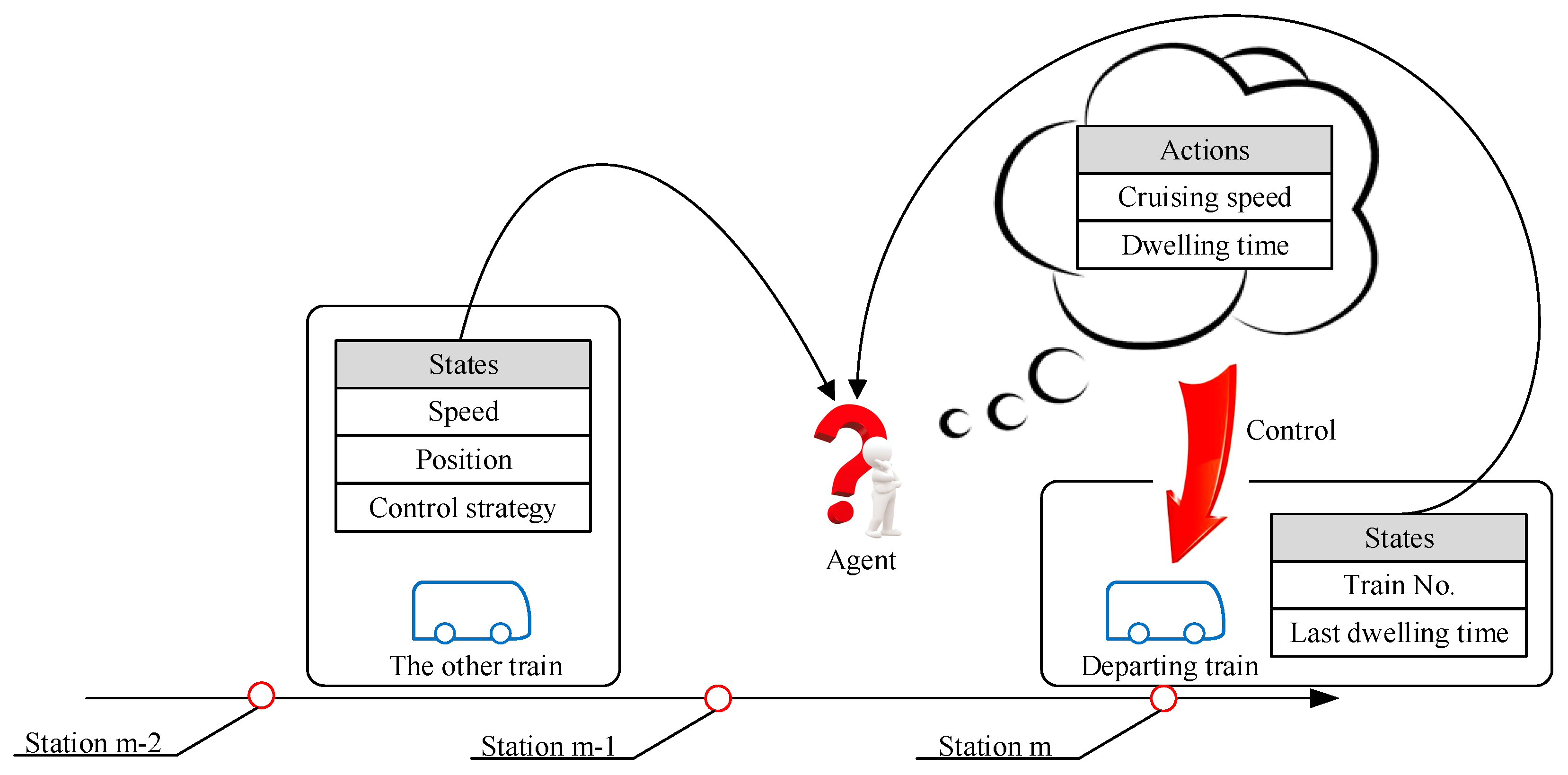
where $\lambda$ is a parameter. Figure 5 shows the sketch map of the DDPG in a two-train network, where the agent is observing the state of trains in the metro network from the environment and thinking which action should be taken for the departing train. The action works on the environment, then the trains get into the next state. During each step, the environment provides a reward to the agent.

5. Experimental Validation

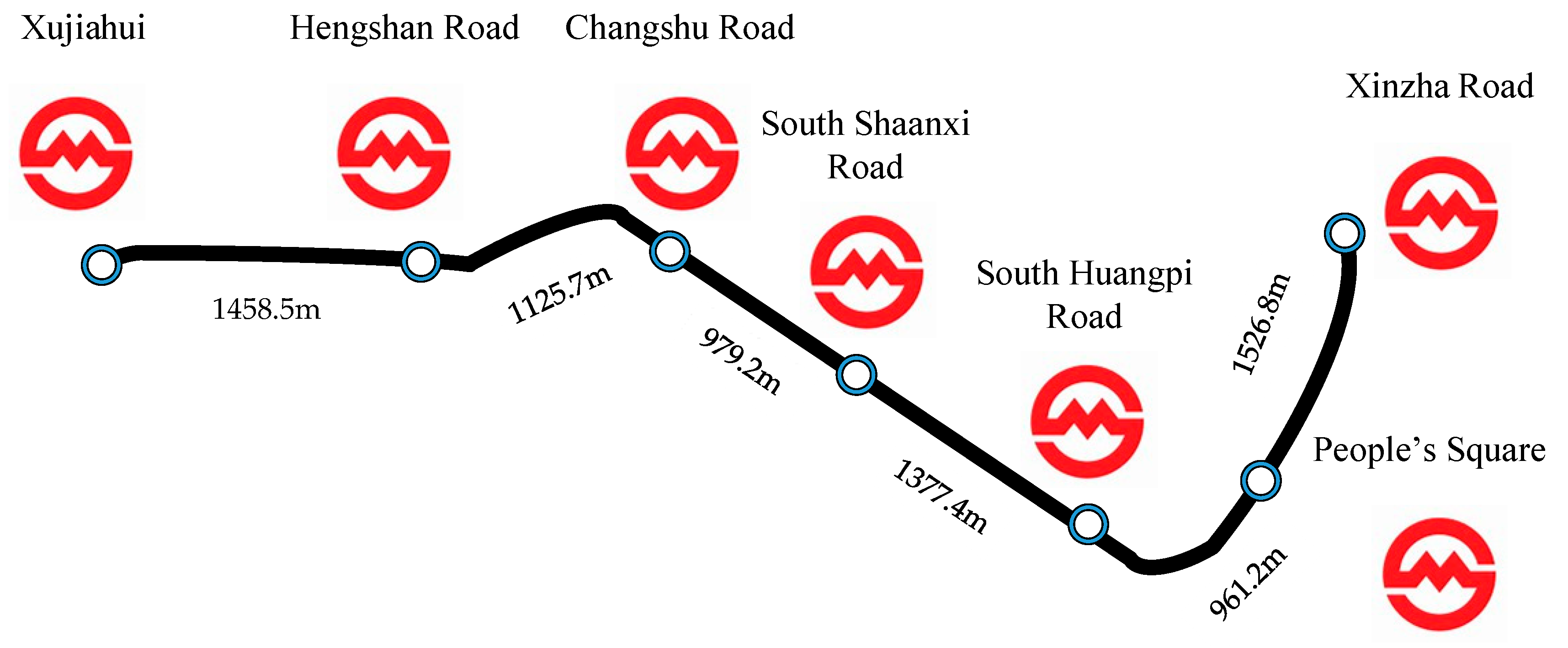
In order to validate DDPG in the ETTR problem, numerical experiments are conducted in the Shanghai Metro Line 1 (SML1), which is one of the oldest metro lines in China. There are a total of 28 stations with a daily ridership of over 1,000,000 passengers [36]. According to the statistical data in daily peak hours, the metro network implements a tight schedule, of which the average traveling time during a section is only 2 min, and the uniform interval time between two trains is 164 s The first three experiments are based on a situation that two trains run on a segment of SML1 from Xujiahui to the Xinzha Road. The last experiment focuses on a three-train network in the same segment. Information of stations and segments are shown in Figure 6.

Experiment 1: The objective of the first experiment is to schedule an offline optimal timetable without any disturbance. The foundation settings are listed as follows. The headway is set as 120 s. The dwelling time consists of a fixed dwelling time and a flexible dwelling time [26]. The fixed dwelling time is set as 20 s while the flexible dwelling time ranges from 10–15 s. The cruising speed is $v_c^{m,n}\in \left[18,22\right]$ m/s. In this setup, the traffic block conflicts [24] will not happen. The genetic algorithm (GA) is used to obtain the optimal cruising speed and the flexible dwelling time at each station for each train. The final optimal result is shown in

Table 1. Optimal selection by GA in the two-train network.

Segment No.	Cruising Speed (m/s)		Station	Dwelling Time (s)
	Train No.1	Train No.2		Train No.1	Train No.2
1	21.6	18.08	Hengshan Road	20	27.1
2	18.88	19.68	Changshu Road	20	29.8
3	19.72	18.4	South Shaanxi Road	20	28.1
4	22	18	South Huangpi Road	22.8	24.8
5	18	18.52	People’s square	21.1	20
6	18	18.04	Xinzha Road	-	-

.

It takes 4325 s to obtain an offline timetable using a PC with Intel i7-4720HQ CPU. This reflects that GA is not suitable for adjusting the timetable in real-time when disturbances happen.

Experiment 2: DDPG is used to adjust the cruising speed and flexible dwelling time, when a disturbance happens at train No.1 on the Changshu Road Station. In this experiment, disturbances are discretely sampled, uniformly selected from a discrete point set $\epsilon \in \left\{11,12,13,14,15\right\}$. The neuronal structure of the actor network is set as $5\times 400\times 300\times 2$, and the neuronal structure of the critic network is set as $7\times 400\times 300\times 1$. In essence, DDPG samples history data from a process that the agent interacts with the environment, and this data is used to update both the actor network and the critic network. The training process is offline, so the total training episode will not affect the real-time performance. The total training episode cannot be too small to search stable rewards, and it cannot be too large that the actor network and the critic network are overfitted. According to the training performance, the total episode is set as 3000.

Table 2. The set of parameters in experiment 2.

Parameters	Values
Memory_capacity	500
Batch_size	10
$\tau$	0.005
$\gamma$	0.1
$\lambda$	20

lists the set of the other parameters in DDPG.

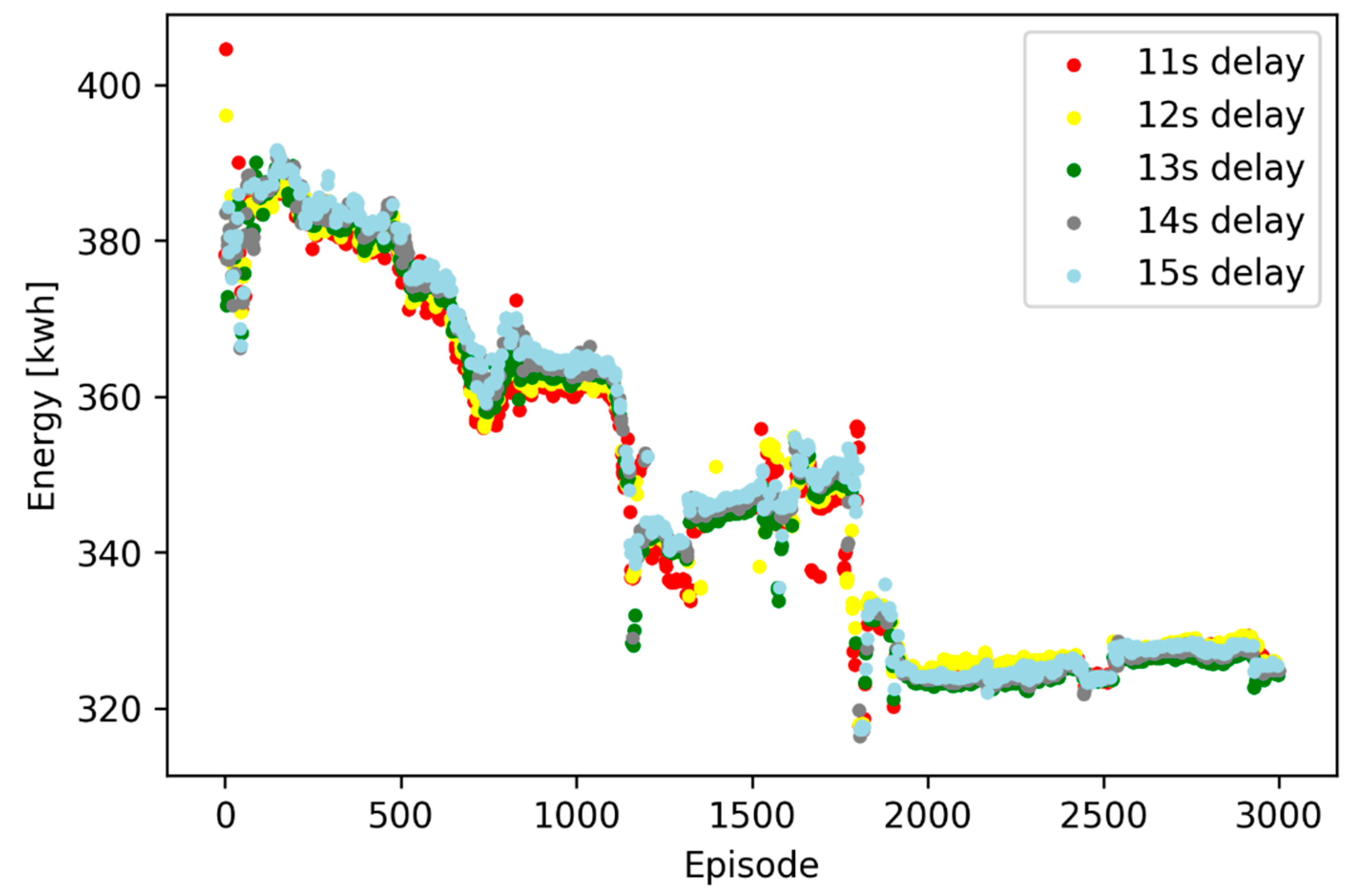
Here, Memory_capacity represents the size of the buffer $R$, Batch_size represents the size of the minibatch $N$, $\tau$ represents the update rates from the current network to the target network, $\gamma$ represents the discount factor, and $\lambda$ is the reward parameter. Figure 7 shows the total energy consumption for each episode, more specifically, the training episodes of DDPG under discretely sampling random disturbances.

As shown in Figure 7, the beginning episodes (between zero and 50) are the exploration process, where the agent has a rapid progress but has not found a proper solution. A similar process happens on the episode 1200 and 1800. During 1200 to 1300 and 1550 to 1750, the agent sinks into the local extremum and energy consumption stays stable. In these situations, the agent can escape from local extremum and search new solutions. After the 2000-episode training, the agent stays stable under different disturbances. 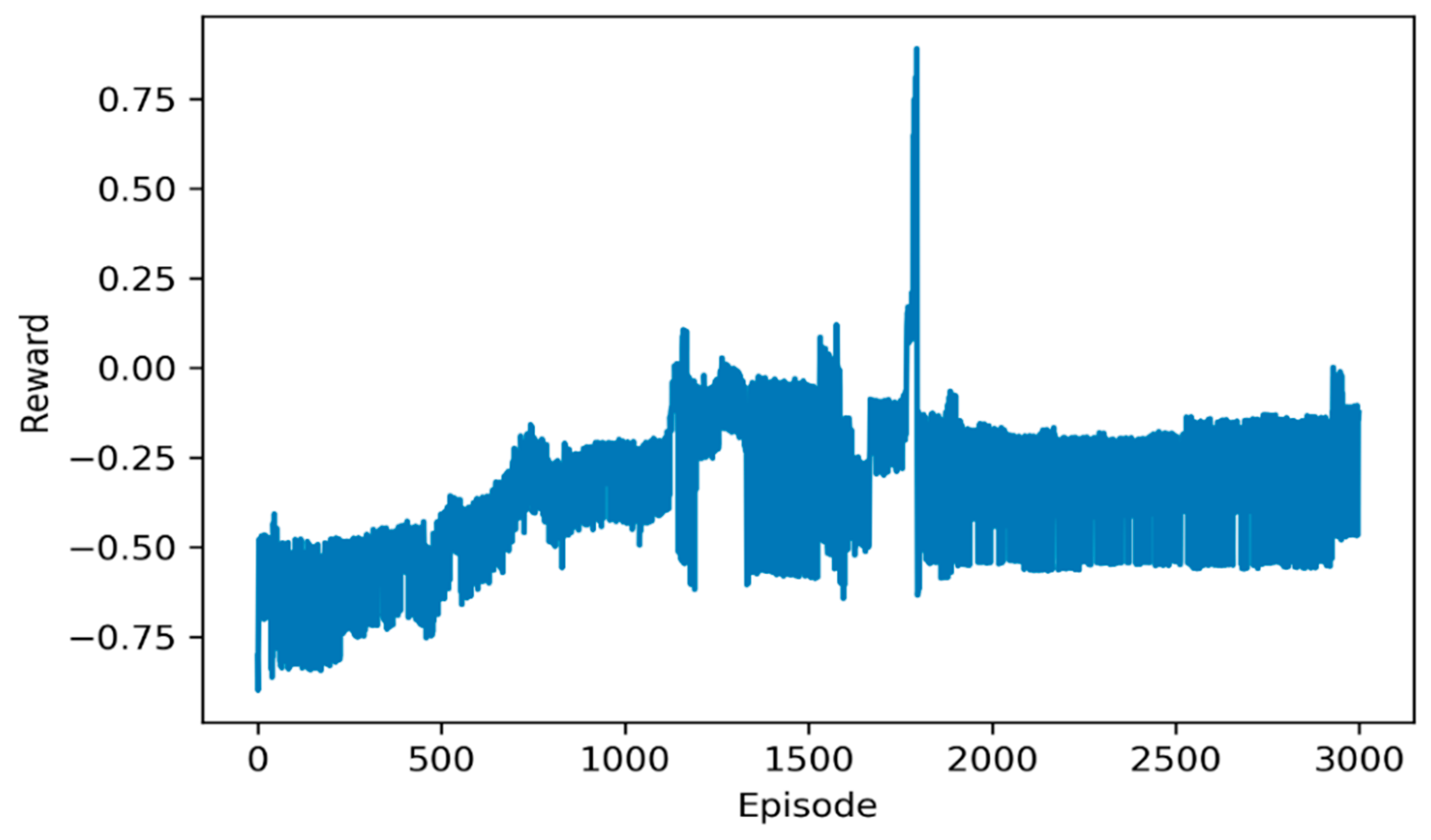Figure 8 shows the rewards during optimization.

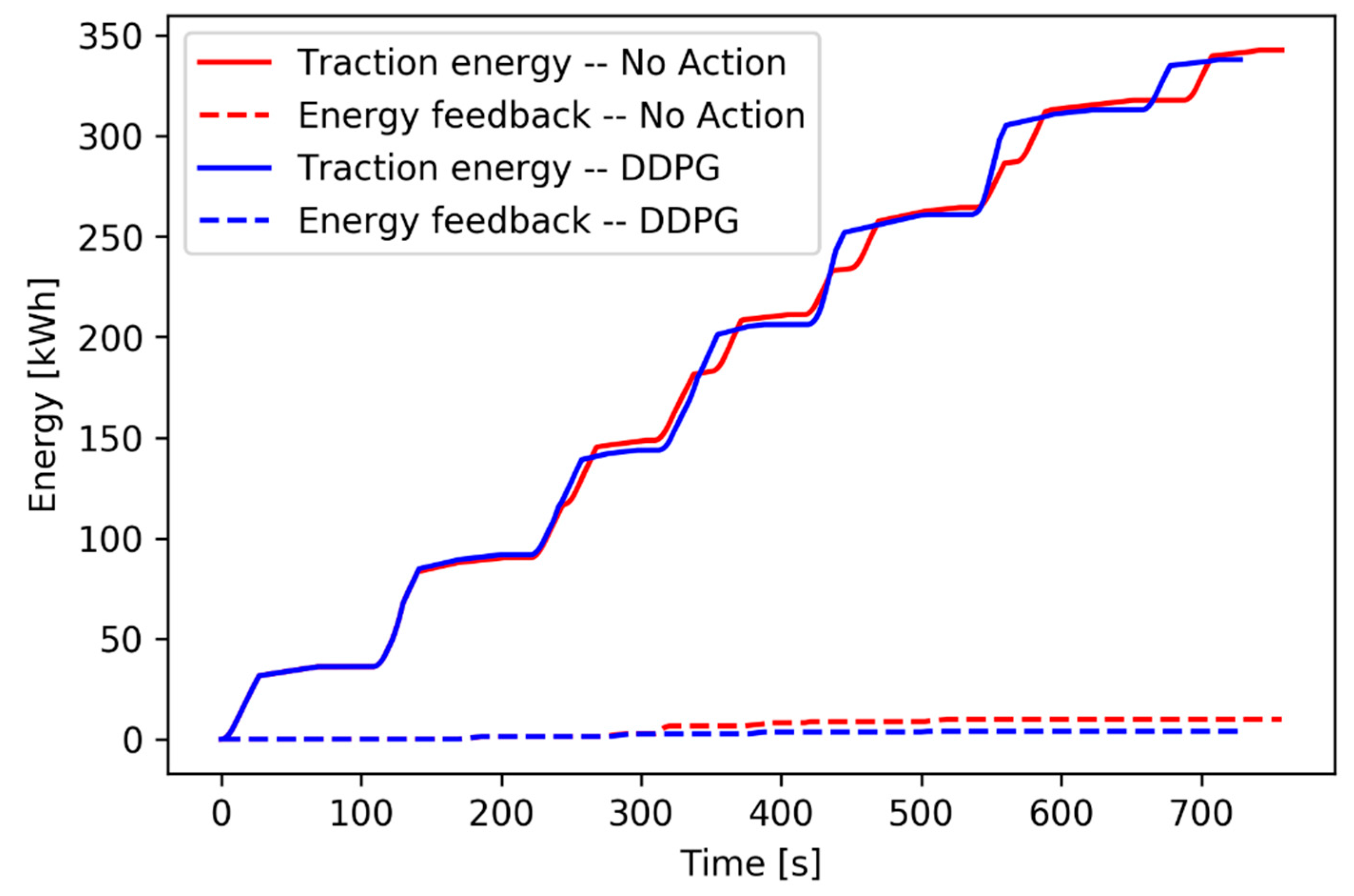
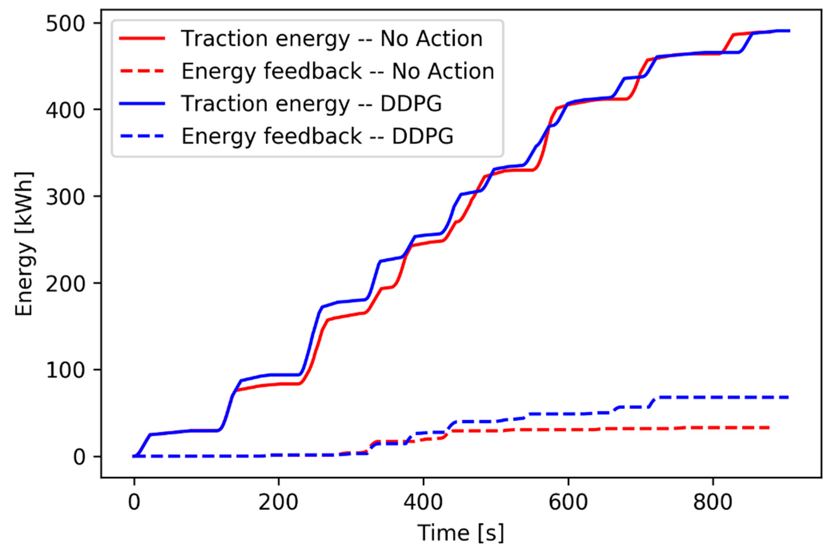
In Figure 8, the reward curve presents an uptrend with the episode increasing, but it is not beyond zero in the final episode. According to the reward function, the reason is obvious that the relative traction energy and the relative feedback energy are cancelled out. In another word, the final reward is not beyond zero, because DDPG saves the traction energy, while wastes the feedback energy. Figure 9 shows the energy accumulation for one episode under an 11 s delay.

Comparison on the traction energy consumption and the energy feedback shows that the agent of DDPG adopts a series of action, which reduces the traction energy but ignore gains in the energy feedback.

The training episodes above only show the trend of the agent searching solutions, but do not validate that it saves energy. Hence, test episodes are implemented.

Table 3. Energy consumption statistics during the training process under discretely sampling random disturbances in the two-train network.

Delay (s)	No Action (kWh)	DDPG (kWh)	Percent of Saving Energy
11	325.25	324.90	0.11%
12	328.31	325.68	0.80%
13	330.71	324.41	1.91%
14	331.81	324.97	2.06%
15	332.80	325.45	2.21%

shows the testing results under different disturbances, with the trained neural networks in Figure 7.

Table 3 shows that, under the larger delay, about 2% energy can be saved, but under the smaller delay, the agent can hardly save energy. On the basis of discretely sampling random disturbances, there are not enough samples supporting the learning of the agent, leading to an unremarkable percentage of energy saving. The experiment reflects that discretely sampling random disturbances cannot train out optimal DDPG networks. Experiment 3 gives a proper solution to promote the learning efficiency of the agent.

Experiment 3: DDPG is used to adjust the cruising speed and flexible dwelling time, when a disturbance happens at Train No.1 on the Changshu Road Station. The disturbance is in the continuous section $\epsilon \in \left[10,15\right]$. The maximum training episode is set as 3800. The structure of the actor network and the critic network are set the same as they are in Experiment 2. Other parameters in DDPG are set as

Table 4. The set of parameters in experiment 3.

Parameters	Values
Memory_capacity	1000
Batch_size	50
$\tau$	0.005
$\gamma$	0.1
$\lambda$	100

.

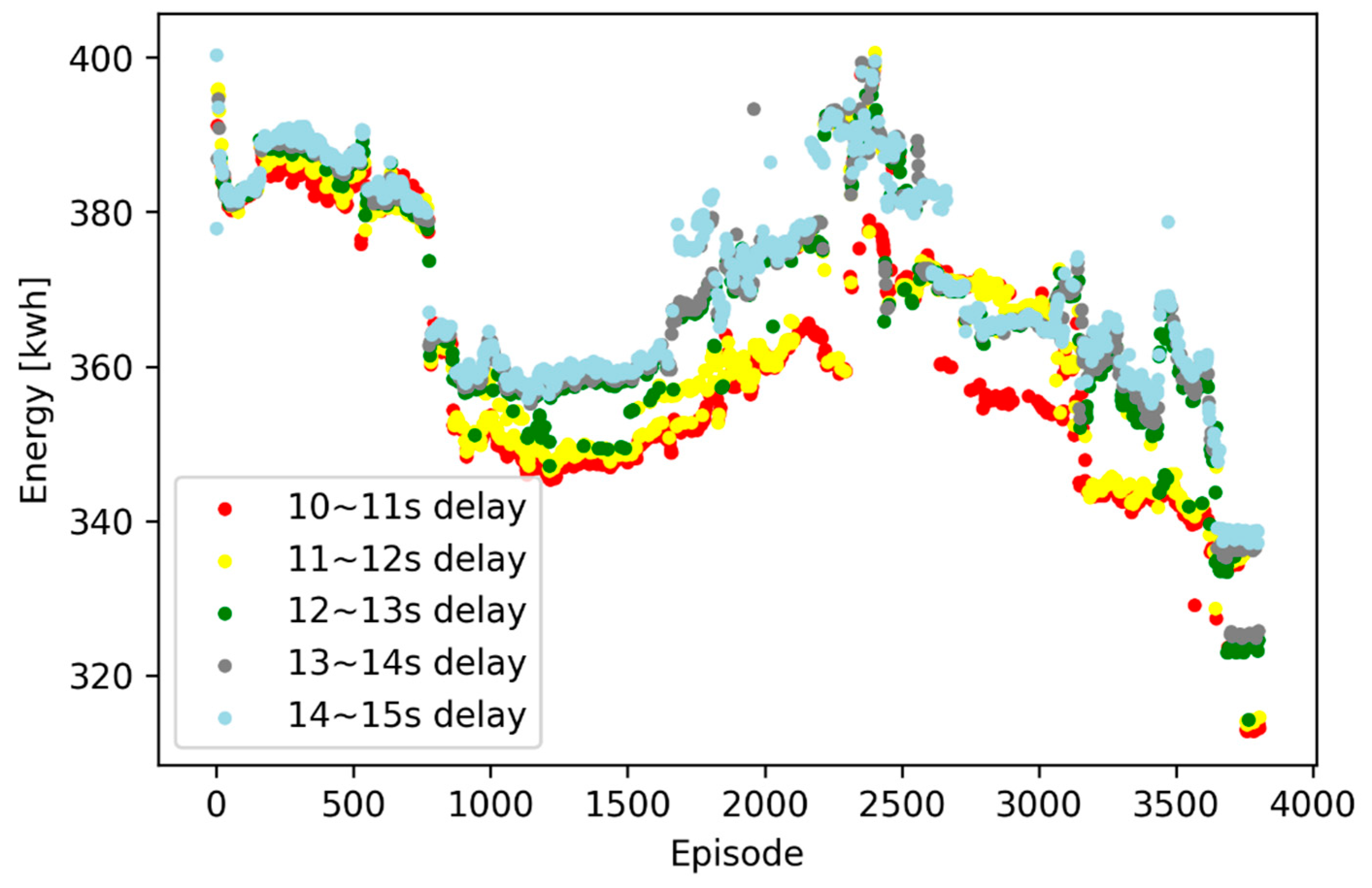
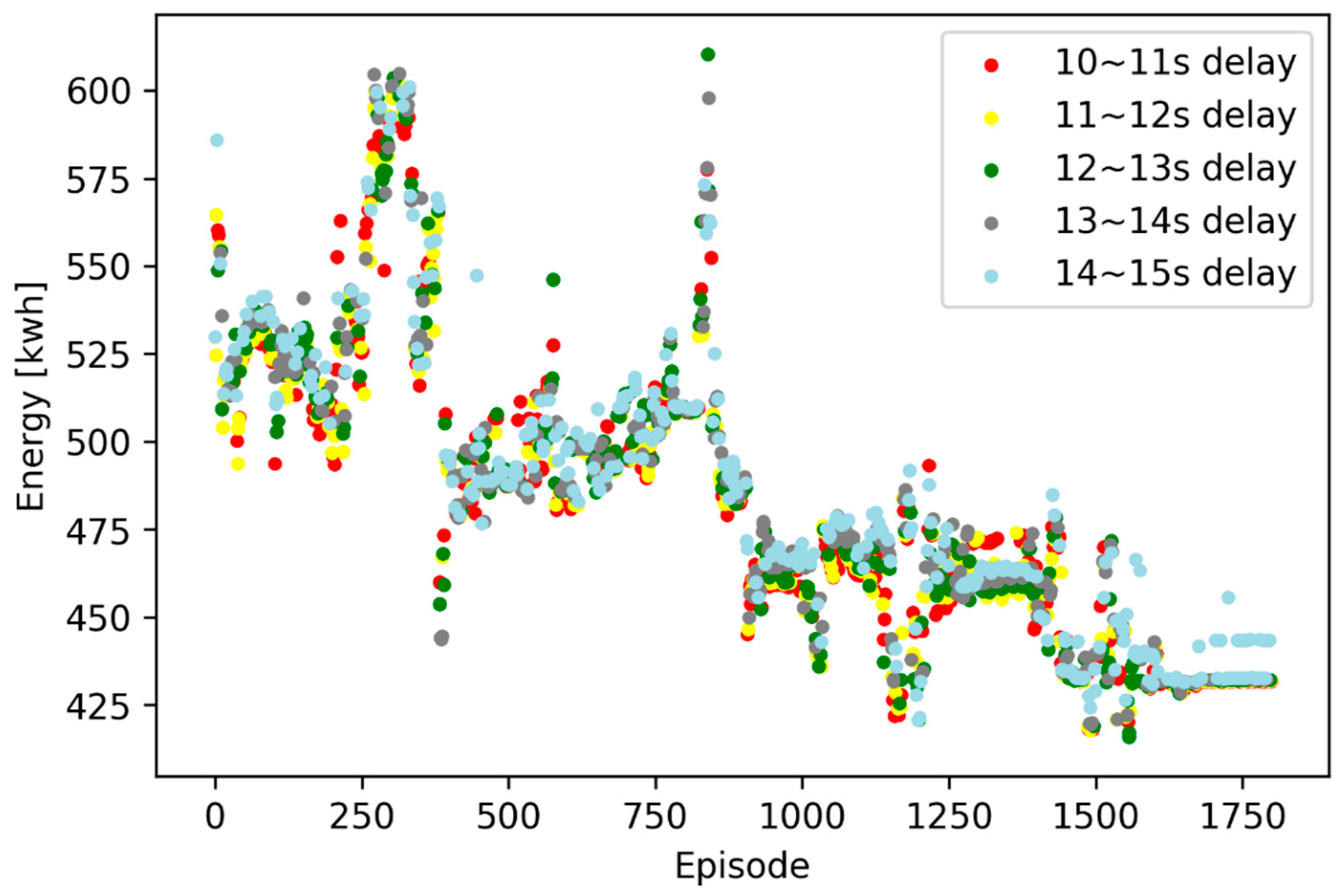
Figure 10 shows the total energy consumption in each training episode under continuously sampling random disturbances by DDPG.

Compared with Figure 7, the convergence speed of the scatters in Figure 10 is slower, and the final performance of energy saving is better. Both the actor network and the critic networks are well trained and the agent is not hovering around the local extremum.

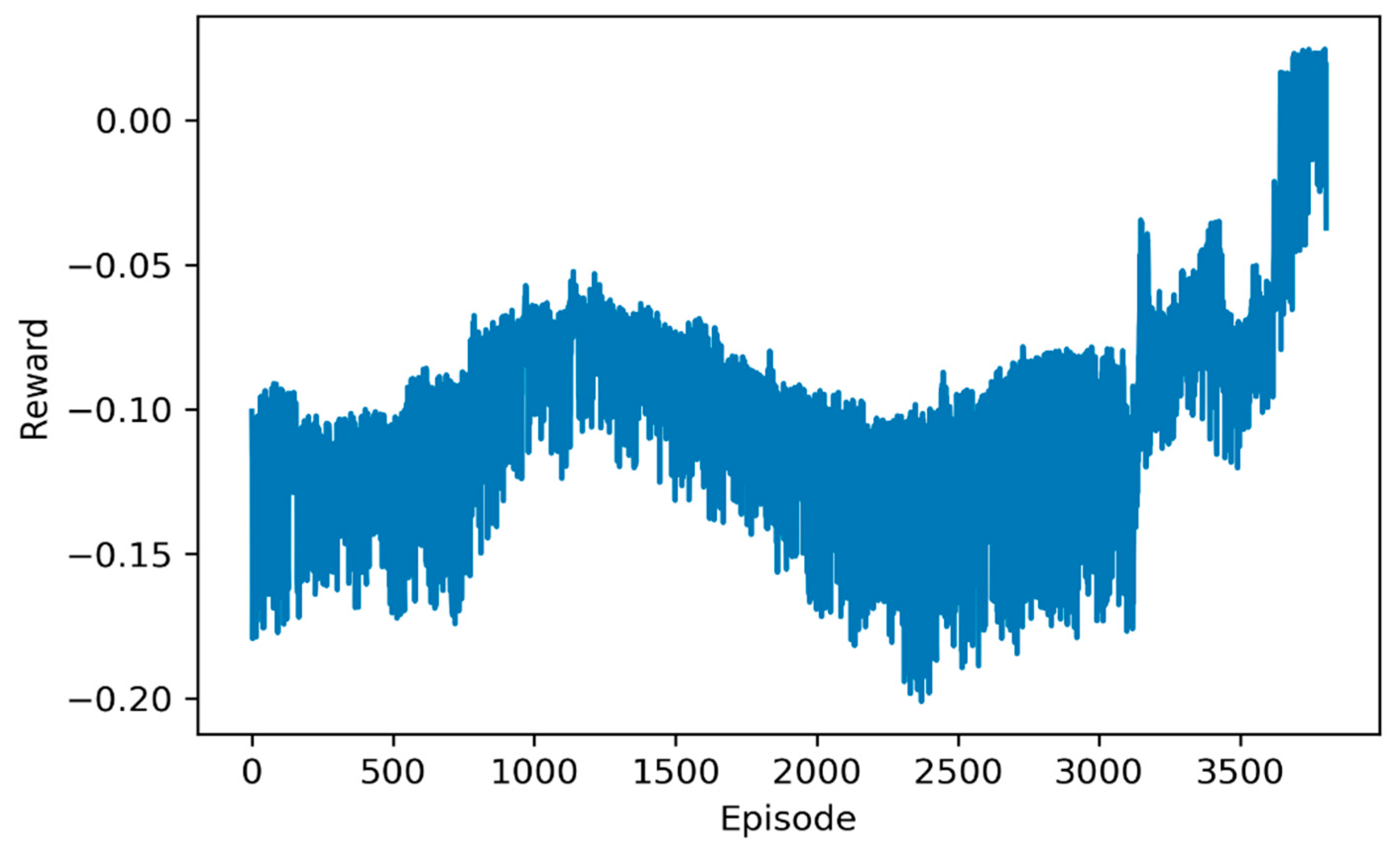
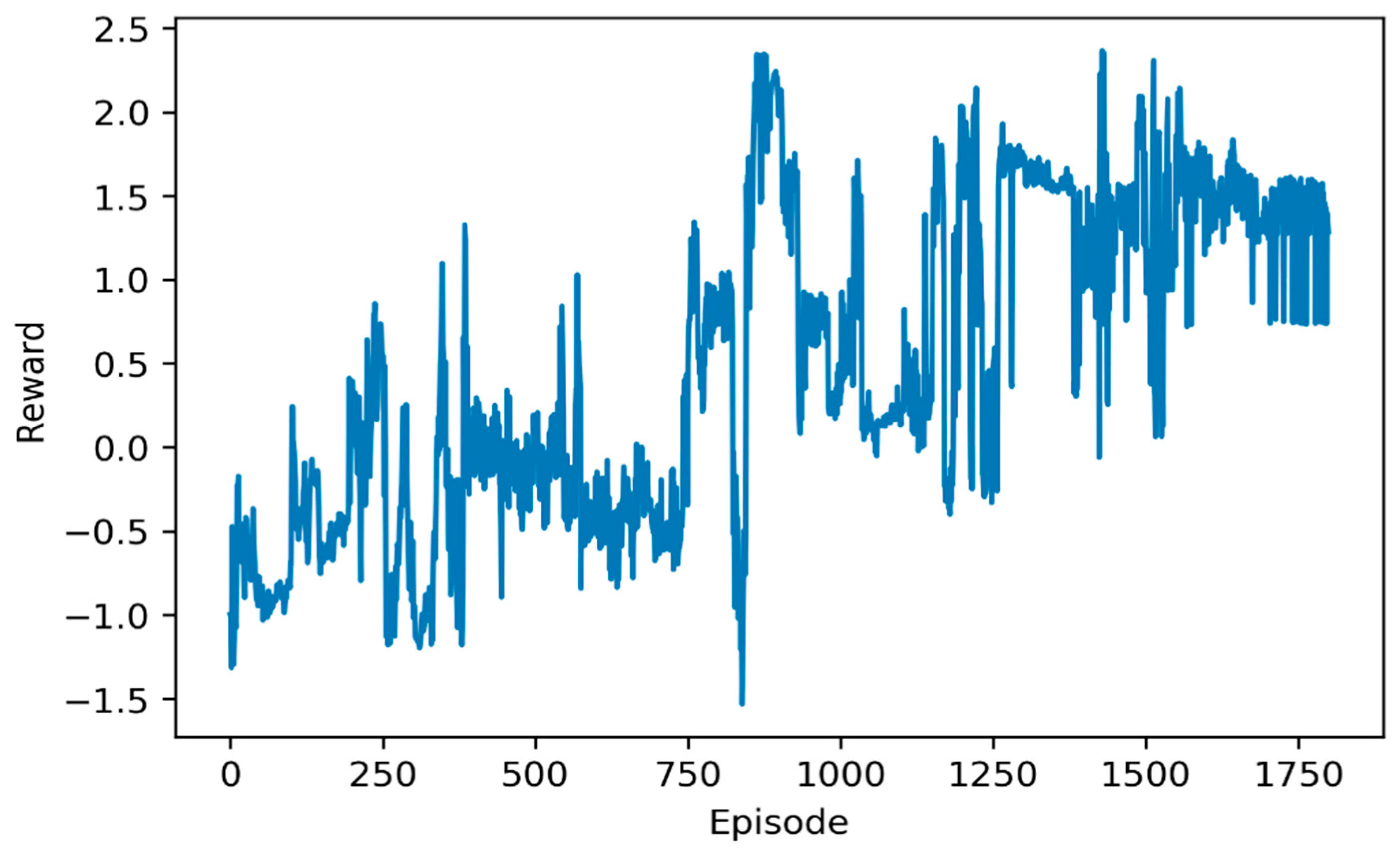
Figure 11 shows the rewards in the training episodes by DDPG. During the 3000 to 3800 episodes, the reward significantly increases, and finally beyond zero.

In the following, testing episodes are implemented, which try to validate that the performance of the agent is as well as it is in the final training episodes, and to validate the real-time characteristic of the well-learned agent.

The testing episodes is set as 10, and the disturbance is also random selected in the uniform distribution that $\epsilon \in \left[10,15\right]$.

Table 5. Energy consumption and average spending time during the testing process under continuously sampling random disturbances in the two-train network.

Delay (s)	No Action (kWh)	DDPG (kWh)	Percent of Saving Energy	Average Spending Time (ms)
12.09	328.49	317.75	3.27%	1.27
13.60	331.36	329.07	0.69%	1.68
10.00	321.24	306.10	3.74%	1.60
10.76	324.43	313.77	4.71%	1.60
11.51	330.59	324.57	2.62%	1.60
12.21	327.05	317.34	2.97%	1.59
10.73	324.15	306.61	5.41%	1.79
14.12	331.90	330.08	0.55%	1.60
14.80	332.59	331.55	0.31%	1.99
12.69	330.02	316.94	3.96%	1.99

shows the total energy consumption for each testing episode and the average time spent for each policy decision.

Compared with Table 3, the DDPG training under random continuous disturbances can save more energy, because the random continuous disturbances provide enough different samples, which promotes the agent to understand the environment. The energy saving percent in the testing episode, which keeps stable in different cases of delay, has a similar distribution with that in the training episode. It indicates that the agent is well learned in the training episodes, and overfitting is not happening in the actor network and the critic network. Compared to GA, DDPG has a natural advantage in terms of the average time spent in each policy decision process. 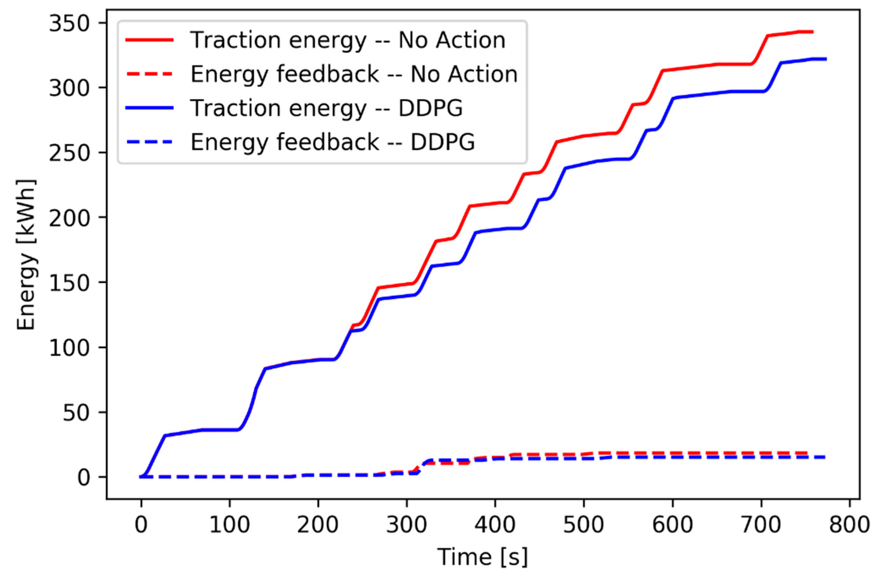Figure 12 shows the energy accumulation for one testing episode under a 10.76 s delay.

As shown in Figure 12, the DDPG agent also chooses to reduce the average speed to save the traction energy. Different from experiment 2, the energy feedback increases from 305 s. This makes the DDPG in this experiment save more energy than before. Although the reward function increases the weight of the energy feedback, reducing the traction energy seems to be bring a higher return for the agent in the two-train network.

For the reason of unremarkable energy feedback in the two-train network, it is essential to take a three-train network for validation.

Experiment 4: DDPG is used to adjust the cruising speed and flexible dwelling time, when a disturbance happens at Train No.1 on the Changshu Road Station. The disturbance is in the continuous section $\epsilon \in \left[10,15\right]$. The maximum training episode is set as 1800. The structure of the actor network and the critic network are set the same as they are in experiment 3. Memory_capacity is set as 500 and $\lambda$ is set as 20, and other parameters in DDPG are set the same as in Table 4. The only difference between experiment 4 and 3 is the number of the running trains. The headway of each train is set as 120 s.

First, an offline optimal timetable is built by GA under no disturbance situation.

Table 6. Optimal timetable by GA in the three-train network.

Segment No.	Cruising Speed (m/s)			Station	Dwelling Time (s)
	Train No.1	Train No.2	Train No.3		Train No.1	Train No.2	Train No.3
1	19.12	18.04	18	Hengshan Road	20.1	29.6	24.5
2	18.8	18	18.2	Changshu Road	21	28.2	20.2
3	20.16	18	19.48	South Shaanxi Road	22.7	20	26.3
4	20.36	18.04	18	South Huangpi Road	20	23.7	29.1
5	18.04	18	18	People’s square	24.2	23.4	26.8
6	19.48	18.12	18	Xinzha Road	-	-	-

shows the selected cruising speed and dwelling time.

Figure 13 shows the total energy consumption in each training episode under continuously sampling random disturbances by DDPG.

According to Figure 13 and Figure 14, during training, energy consumption is fluctuated in a downward trend and rewards climb up and beyond zero. The final episode is not the minimum point, but it is a stable point under different disturbances.

Table 7. Energy consumption and average spending time during the testing process under continuously sampling random disturbances in the three-train network.

Delay (s)	No Action (kWh)	DDPG (kWh)	Percent of Saving Energy	Average sPending Time (ms)
12.09	452.77	422.26	6.74%	2.85
13.60	456.16	422.56	7.37%	2.42
10.00	448.04	421.75	5.87%	2.05
11.51	451.59	422.06	6.54%	2.37
10.73	449.94	421.85	6.24%	2.11
10.46	449.44	421.81	6.15%	2.37
10.93	450.34	421.90	6.32%	2.06
11.72	452.02	422.13	6.61%	1.93
11.98	452.55	422.22	6.70%	2.11
12.69	454.07	422.34	6.99%	2.11

shows the performance of the agent in the testing episodes. As shown in Table 7, the agent saves energy ranging from 5.87% to 7.37% under different disturbances. Moreover, the time to obtain an action is only 2.23 ms on average, which indicates that DDPG still has a real-time feature in the three-train network. Compared with the two-train network, DDPG saves more energy in the three-train network.

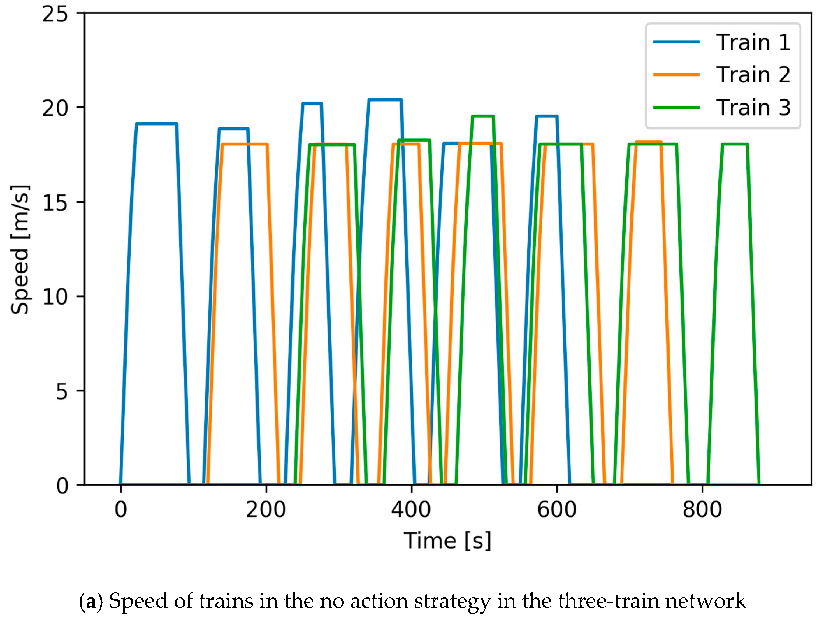
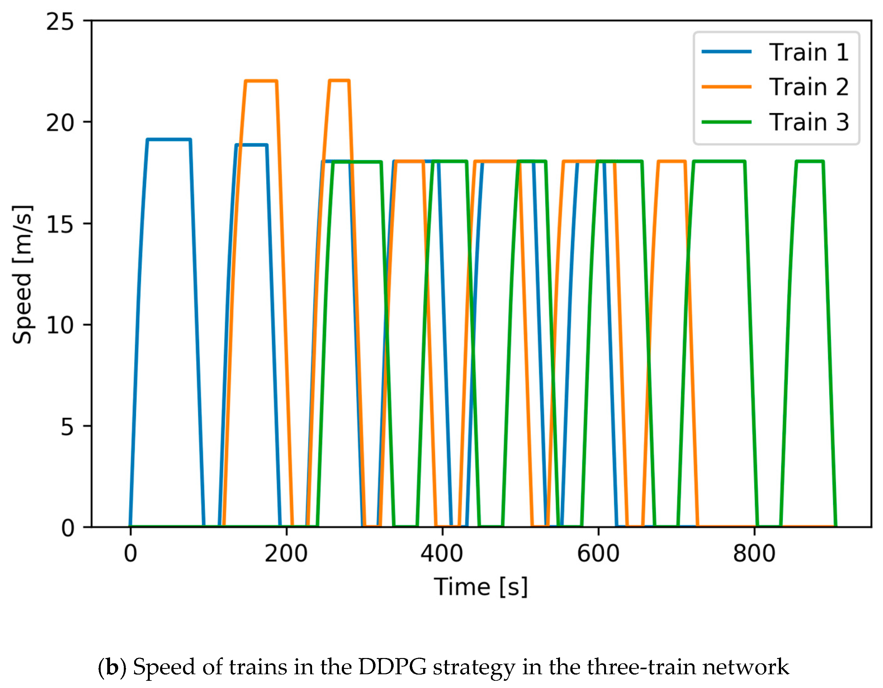
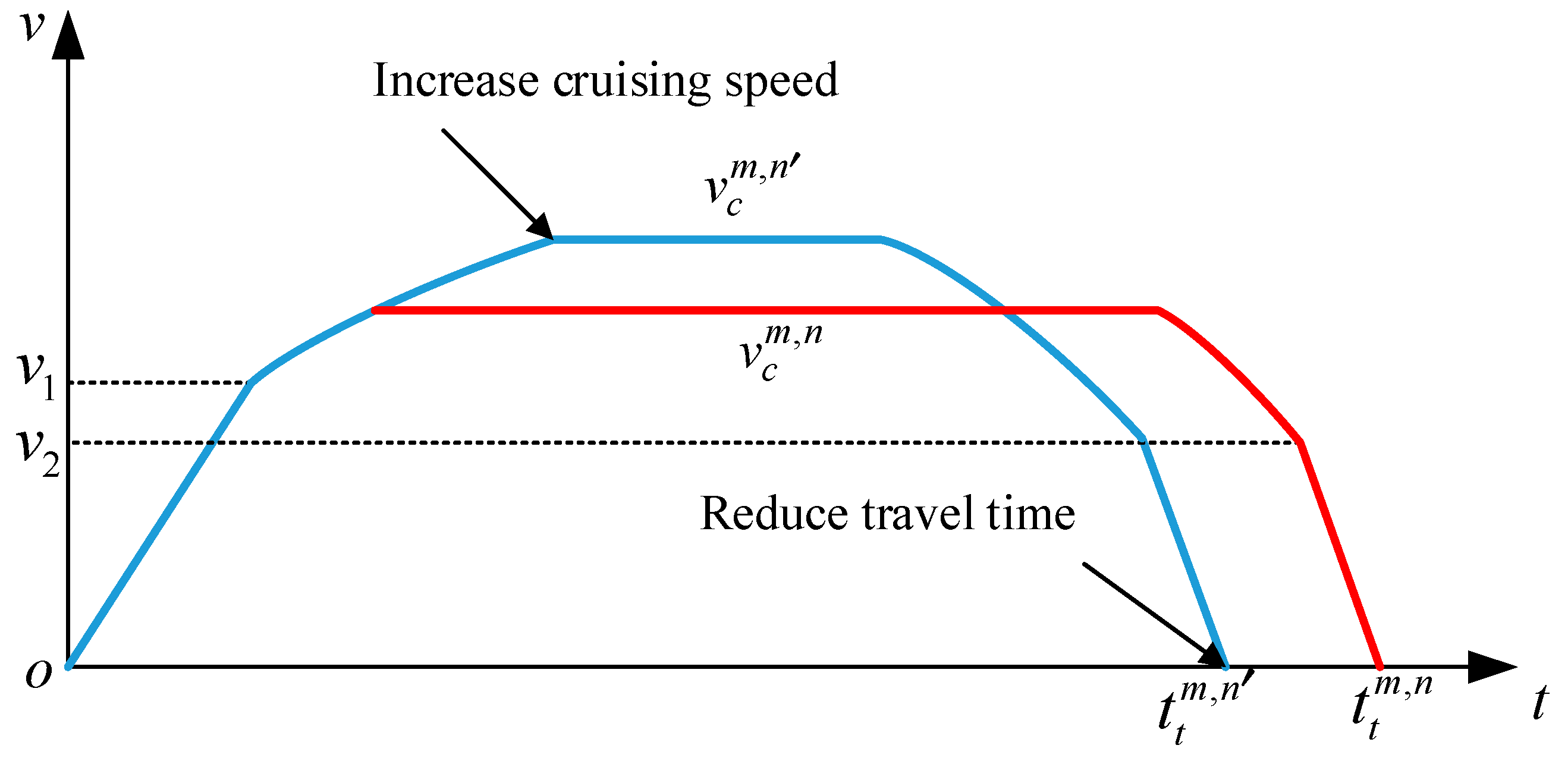
Figure 15 shows the speed curves under a 13.60 s delay in the three-train network, in which Figure 15a shows the speed of trains in the no action strategy and Figure 15b shows the speed of trains in the DDPG strategy. DDPG raises the cruising speed of train No.2 in the first two interstation, and adjusts the dwelling time to synchronize acceleration and braking, which maximizes the feedback energy. DDPG also reduces the cruising speed in other interstations of train No.2 and the cruising speed of other trains to reduce the traction energy.

Figure 16 shows the traction energy and the energy feedback under a 13.60 s delay, which indirectly reflects the effects of the reward function in the three-train network.

As shown in Figure 16, the reward function weights the energy feedback and the traction energy, which forces the agent tending to promote the energy feedback in priority. The blue solid curve shows that DDPG cannot save more traction energy in the three-train network. However, as shown by the dotted lines, this algorithm saves considerable energy on the energy feedback. In terms of total effects, the provided strategy effectively saves more energy in the three-train network.

6. Conclusions

In this paper, a deep deterministic policy gradient algorithm is applied in the energy-aimed timetable rescheduling problem by rescheduling the timetable after disturbances happen and maximizing the regenerative energy from the braking trains. As required by the ETTR problems, DDPG reschedules the timetable in real-time to avoid the chain reactions and saves more energy, and provides a proper cruising speed and dwelling time adaptively under random disturbances.

Superior to the Q-learning algorithm, the observations of DDPG such as the speed and the position of trains are continuous, and the targets such as the cruising speed and the dwelling time are continuous as well. This algorithm can deal with random continuous disturbances, and take continuous action, which is unable to be achieved by the Q-learning algorithm.

GA is suitable for building an offline timetable without disturbances. However, it is not suitable for the ETTR problem for taking too much computation time (4325 s in the above experiment) to obtain an offline timetable for the two-train network. By comparison, DDPG has real-time features for the neural network structure. During the testing episode under the random continuous disturbances, it takes a very short time, ranging from 1.27 ms to 1.99 ms, to choose a pair of proper action.

The proper training mode will improve the performance of DDPG. According to the experimental studies on the Shanghai Metro Line 1, the agent trains under discretely sampling random disturbances, and saves energy from 0.11% to 2.21%. By comparison, the agent performs better after the training under continuously sampling random disturbances, which saves energy from 0.31% to 5.41% in the testing episodes. DDPG can also be used in the three-train network. It takes 2.23 ms on average to obtain a pair of proper action, and the rate of the saving energy ranges from 5.87% to 7.37%.