Article

Knowledge Embedded Semi-Supervised Deep Learning for Detecting Non-Technical Losses in the Smart Grid

1
State Grid Jiangsu Electric Power Co., Ltd. Research Institute, Nanjing 210019, China
2
State Grid Key laboratory of Electrical Power Metering, Nanjing 210039, China
3
State Grid Nanjing Power Supply Company, Nanjing 210000, China
4
School of Electronic Information and Communications, Huazhong University of Science and Technology, Wuhan 430074, China
*
Author to whom correspondence should be addressed.
Energies 2019, 12(18), 3452; https://doi.org/10.3390/en12183452
Submission received: 23 July 2019 / Revised: 3 September 2019 / Accepted: 5 September 2019 / Published: 6 September 2019

Abstract

:
Non-technical losses (NTL) caused by fault or electricity theft is greatly harmful to the power grid. Industrial customers consume most of the power energy, and it is important to reduce this part of NTL. Currently, most work concentrates on analyzing characteristic of electricity consumption to detect NTL among residential customers. However, the related feature models cannot be adapted to industrial customers because they do not have a fixed electricity consumption pattern. Therefore, this paper starts from the principle of electricity measurement, and proposes a deep learning-based method to extract advanced features from massive smart meter data rather than artificial features. Firstly, we organize electricity magnitudes as one-dimensional sample data and embed the knowledge of electricity measurement in channels. Then, this paper proposes a semi-supervised deep learning model which uses a large number of unlabeled data and adversarial module to avoid overfitting. The experiment results show that our approach can achieve satisfactory performance even when trained by very small samples. Compared with the state-of-the-art methods, our method has achieved obvious improvement in all metrics.

Graphical Abstract

1. Introduction

Non-technical losses (NTL) are one of the most major problems pertaining to the power grid, and have been for quite a long time. Unlike technical losses which are generally caused during generation and distribution, NTL are anomalies which include installation errors, faulty meters and electricity theft, etc. Referring to World Bank reports, NTL represents a significant part of the total power losses in both developing and developed nations [1]. A survey from the Northeast Group LLC shows that more than $89.3 billion is lost every year worldwide due to NTL [2]. Besides financial losses, NTL also causes a decrease of stability and reliability of the power grid.
Presently, over 80% of the global population has access to electricity [1]. However, in total electricity consumption, industrial and large commercial customers contribute approximately 55% in Spain [3]. Similarly in China, the ratio of industrial customers is more than 65% [4]. Naturally, detecting NTL among industrial customers is more interesting than residential customers to electricity providers. Hence, this paper aims to detect NTL among industrial customers.
Conventional NTL detection methods depend on the in-field inspection, where both the costs and efficiency can not satisfy electricity providers. With the appearance of the smart grid comes a great deal of smart meter (SM) data and extra opportunities to solve NTL. Hence, a lot of data oriented methods have been proposed recently, due to the development of machine learning and ease of implementation [5]. Researchers adopt methods of different fields of knowledge with machine learning, such as anomaly detection, cybersecurity, etc. Generally, these approaches can be classified as supervised, unsupervised and ensemble methods. Through studying anomaly behaviour in electricity consumption, some of them can help to identify NTL indeed [6]. However, they only got better effect on residential customers rather than industrial customers. The primary reasons are listed as follows:
  • The consumption pattern of residential customers is more stable than that of industrial customers. It is easier to find change points of residential consumption history, while industrial customers have multiple consumption patterns because they have to adjust their consumption behaviour according to the market [7].
  • Residential customers are similar to each other, while industrial customers are quite different. It is easier to cluster residential customers into limited categories [8]. Particularly, [9] uses the location as assistant feature. On the contrary, industrial customers’ consumption patterns are quite different from one another, even if they belong to the same domain or are located near to each other [3].
Therefore, it is more difficult to detect NTL only depends on electricity consumption among industrial customers. The key challenges are reflected on the follows:
  • How to extract features with higher linear separability? Refer to recent research, the features are mostly designed manually according to observation and experience based on electricity consumption. They can hardly represent all scenarios of NTL because consumption behaviour is random and unpredictable, especially for industrial customers. For example, when changes in consumption pattern due to change in household residents or usage of electrical devices might make it looks like electricity theft [10]. This situation would destroy linear separability of traditional features.
  • How to obtain satisfactory performance based on limited labeled samples? Compared to unsupervised learning-based methods, supervised learning-based methods acquired better detection accuracy and become used in the mainstream gradually. However, the realistic NTL samples of which in-field inspected are rare indeed, supervised learning methods are an easier lead to overfitting. On the other hand, the artificial samples as a possible solution are adopted by some approaches [10,11]. Even though they provide lots of labeled samples to support training models, the effectiveness of such attack models is not verified by realistic cases. Due to preconfigured parameters or fixed distribution, it is believable that such artificial samples would also lead to overfitting easily.
  • How to achieve higher accuracy among various customers? Currently, many of related approaches which are based on Support Vector Machines (SVM), K-Nearest Neighbors (KNN), etc., have low accuracy. Even if using much auxiliary data [3] or a large number of labeled samples [12], the performance of these approaches still cannot suit realistic requirements.
Therefore, this paper proposes a deep learning-based Semi-Supervised AutoEncoder (SSAE) model, and attempts to solve the above problems and achieve an ideal NTL recognition accuracy. In this work, we focus on three-phase industrial customers with a contracted power higher than 80 kVA. We design a deep semi-supervised neural network to learn advanced features from massive SM data includes voltage, current, active power, etc. The extracted features cover both principle of electricity measurement and consumption behavior through knowledge embedding. Our model has been trained, validated and tested using real in-field inspected data. Overall, the main contributions of this paper can be summarized as follows:
  • Based on SM data, this paper designs a domain knowledge embedded data model to enhance linear separability of normal samples and abnormal samples.
  • We propose a novel deep neural network-based semi-supervised model to extract advanced features from limited labeled samples efficiently. In addition, by designing an adversarial module, our model has stronger anti-noise ability.
  • Our approach improves the performance of NTL detection obviously. Experimental results show that all metrics of SSAE model outperform other existing approaches in realistic cases.
The remainder of the paper is organized as follows. Section 2 presents a brief overview of NTL detection. Section 3 presents the problem analysis and introduces knowledge embedded data model. Section 4 presents deep semi-supervised model. Experiments are conducted and the evaluation results are shown in Section 5. Finally, we provide conclusions and future work in Section 6.

2. Related Work

The recent research for NTL detection is around hardware or non-hardware solutions. Due to hardware based solution needing further special sensors, the cost and efficiency can hardly satisfy electricity providers even if it has higher accuracy [12]. With the growing of the smart grid and implementation of advanced metering infrastructure (AMI) systems, electricity providers collect and hold various and massive SM data. Hence, non-hardware solutions are more acceptable to electricity providers, especially data oriented methods. Hence, this section only presents a brief survey of the state-of-the-art on data oriented NTL detection methods.
According to implemented machine learning algorithms, data oriented methods could be roughly categorized into three types:
  • Supervised learning-based methods. They mainly include Decision Tree (DT) [13,14], Support Vector Machines (SVM) [13,15,16], K-Nearest Neighbors (KNN) [17], Bayesian Networks (BN) [18], Artificial Neural Network(ANN) [12,17], Deep Neural Network(DNN) [12], etc. Depend on supervised learning algorithm and artificial feature, these methods acquire satisfactory effect in some situations. Due to the variety of NTL, especially electricity theft, these methods require large samples with the right labels to train algorithms. However, it is difficult to collect enough realistic normal and abnormal cases, which makes the labeled samples are very scarce. To avoid insufficient realistic NTL samples, [10,11,13] attempt to model NTL and produce artificial NTL samples. Same as the necessary requirement of massive labeled samples, features are equally important to classifiers. To construct powerful feature models, most researchers applied raw data, statistics, Fourier coefficients, wavelet coefficients, slope of consumption curve, etc. However, all of them still could not cover all situation of NTL, especially the NTL of industrial customers. Hence, [12] proposed deep learning-based method and self-learned features from massive consumption data. The results from [12] show that wide and deep convolutional neural networks has strong feature learning ability and improve accuracy in electricity theft detection. However, the limitation of consumption data blocks the implementation of [12] to industrial customers.
  • Unsupervised learning-based methods. To avoid labeling massive samples, some researchers choose unsupervised methods to detect NTL. Unsupervised methods do not need any labeled samples, and primary contain clustering [8,19], outlier detection [20] and expert systems [21]. Even though a series of unsupervised methods are free from labeling training set, their performance always could hardly satisfy electricity providers when they deploy standalone. Frequently, unsupervised algorithms pose auxiliary methods. They are used to group similar consumers, and then train further classifiers on these groups [8,19]. However, because of the fact that abnormal samples are always far less than the normal samples, it is still difficult to promise that each group own enough labeled samples. Hence, misjudging tends to occur whatever clustering or classification.
  • Semi-supervised learning-based methods. They allow the NTL detector to be trained on a few labeled samples and large unlabeled samples [22]. In ref. [23] uses Transductive SVM(TSVM) to build a NTL detecting system. Restricted to TSVM could not handle imbalance situation, [23] has not been demonstrated enough for detecting NTL. However, semi-supervised learning still is competitive and hopeful choice for detecting NTL when it meets deep learning.
Summary, most proposals meet following limitations: (1) Electricity consumption is not enough to classify normal and abnormal cases in all possible scenarios; (2) Artificial NTL samples are different from realistic cases and lose effect on industrial customers; (3) Performance of these methods still needs to be greatly improved.
In the recent years, the field of machine-learning has produced several pivotal advances that address complex problems. Deep learning simulates the brain’s structure with multiple layers of neurons, fitting complex functions, and characterizing the input data’s distribution, has demonstrated excellent capacity of automatically learning features. It is widely adopted in computer vision [24], speech-recognition [25], natural language processing [26], etc. and has achieved huge success. Simultaneously, a sequence of semi-supervised deep learning models [27,28,29] have been proposed. It is demonstrated that they had achieved remarkable success in image classification tasks. So, great potential exists that deep learning would contribute a lot to NTL detection application, the research about which is just in the beginning phase.
The electrical magnitudes are great different from data which they handled. Firstly, electrical magnitudes are consisting of multiple time series data, such as voltage, current, etc. Secondary, the dimension of electrical magnitudes is significantly different from image and audio. Furthermore, the knowledge has been naturally embedded in the picture or audio, however, electrical magnitudes do not contain any domain knowledge. Therefore, this study attempts to propose a novel semi-supervised deep learning model to overcome the limitations of the above existing works and detect NTL accurately.

3. Modeling Samples with Knowledge

Although deep learning has strong feature learning ability, it is still difficult to learn domain knowledge from raw data. Hence, this section will provide an efficient way to embed knowledge of electricity measurement into sample model to help deep neural network to extract advanced features.

3.1. Principle of Electricity Measurement

Most industrial customers equipped with three-phase smart meters. According to the different wiring modes, it can be divided into two types: three-phase four-wire and three-phase three-wire. In this paper, we primary introduce our approach with three-phase four-wire as an example. For single phase scenario, the electricity energy is calculated by following equation:
E = n = 0 N 1 P n · Δ t
where, Δ t is the cycle of computation, E is the active electricity energy in a certain time period N · Δ t , P n is the average active power at time n. It can be further calculated by voltage and current:
P n = U n · I n · c o s ϕ n
where, U n and I n are average voltage and current at time n, ϕ n is the phase difference between voltage and current at the same time stamp and c o s ϕ n is called power factor. Further, the equation of active energy are rewritten by:
E = n = 0 N 1 [ U n · I n · c o s ϕ n ] · Δ t
For three-phase four-wire situation, the total active electricity energy is calculated by:
E t o t a l = n = 0 N 1 P t o t a l · Δ t = n = 0 N 1 [ P A n + P B n + P C n ] · Δ t
Generally, electricity energy measured by voltage and current, and the relationship between them is very important to NTL detection.

3.2. SM Data

Due to industrial customers contribute most electricity consumption, electrical providers equipped AMI system to read, collect and save important electricity magnitudes. These magnitudes are read every 15 min and all of them share the same time-stamp. Based on Equations (1)–(3), this paper collects part of them as dataset to train, validate and test the model from State Grid Corporation of China(SGCC) which listed in Table 1. The SM data are labeled manually refer to the result of in-field inspection. The rule for data labeling is that all data of each customer has the same label. There are few label noise in our data set because abnormal customers were not always abnormal.

3.3. Analysis of NTL

The collected SM data reflects the electricity consumption at a certain moment. For normal situation, SM data must follow the principle of electricity measurement mentioned above. On the contrary, anomaly SM data must break the regular law to reduce consumption randomly. Refer to the principle of electricity measurement, the primary types of NTL include:
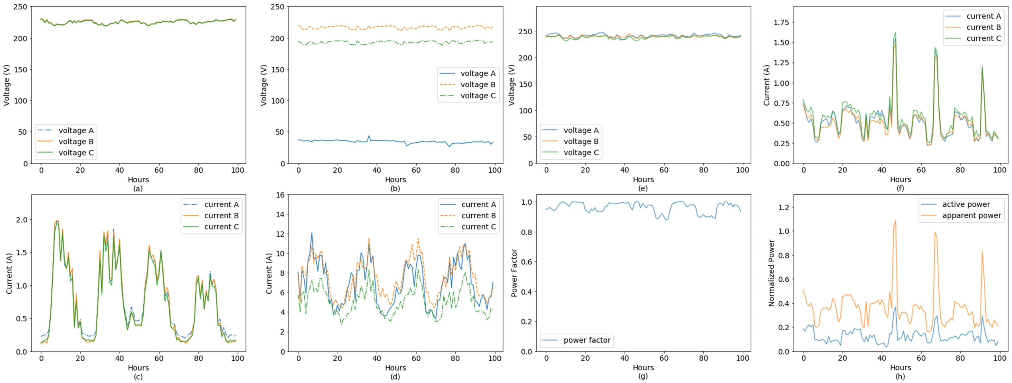
  • Shunts: For a three-phase situation, the shunts is the outputs of PT or CT are shorted or injected a low-resistance path. In general, it would reduce the measured voltage or current. Commonly, voltages and currents of three-phase customers are almost balance [30], such as Figure 1a,c. The shunts will break the balance on voltages or currents, such as Figure 1b,d. In particular, the degree of imbalance about three-phase currents is related to customers’ load level, and is different among all customers. Shunts are the most complicated NTL because normal customers may also have similar phenomenon. In Figure 1c, the currents of a normal customer also have little imbalance when the load is low.
  • Phase Shift: It means that the phase difference between voltage and current is changed artificially. Through increasing ϕ to reduce the power factor, and decrease the measured active power. There is a significant phenomenon that the power factor reduced obviously. Commonly, the power factor should close to 1.
  • Phase disorder: The currents are coupled with the wrong voltages. Figure 1e–h presents a typical example of this case. The output of phase-A’s CT and PT are jointed mistakenly with the output of phase-B’s PT and CT. From the curves of Figure 1e–g, it can be found that the voltages and currents and power factor are almost normal respectively. However, there is a large gap between measured total active power and estimated total apparent power in Figure 1h.
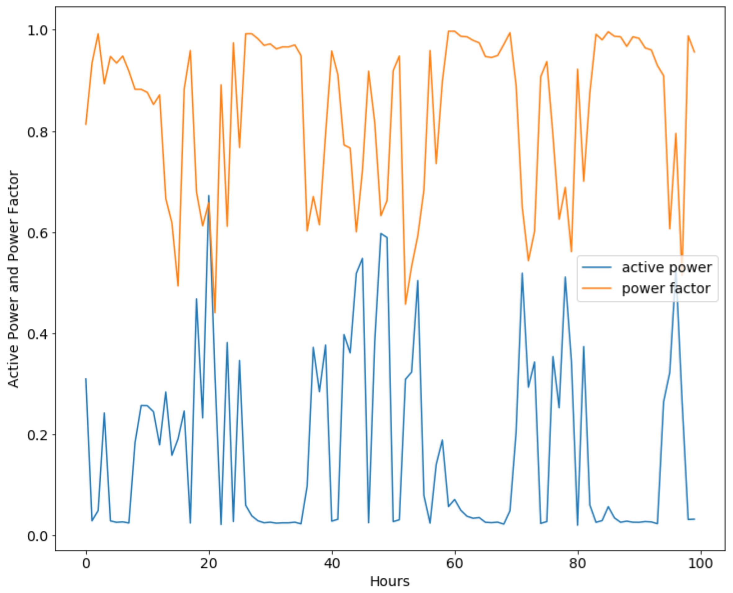
  • Phase Inversion: The phase of voltage or current is inverse directly. The phase difference between voltage and current is changed from ϕ to ( π ϕ ) . The smart meter will measure a negative active power of such wire and smaller total active power. Figure 2 shows a more complicated situation, all phases are inversion. This time, there is no abnormality in SM data, too. However, when we analyze active power and power factor jointly, it can be found that they are negative related rather than positive related.
Overall, it is difficult to discover NTL among industrial customers only with SM data because the pattern of NTL mentioned above will be changed timely and randomly. Furthermore, it might be existed from the beginning, such as phase disorder. In contrast to the SMART attack defined in [11] or FDI5 defined in [10], the realistic NTL does not run in fixed artificial model and is more random and complicated. Consequently, the domain knowledge based features are very important for classifier to detect NTL.

3.4. Sample Model with Knowledge Embedding

Before starting to train a deep neural network (DNN), it is necessary to model SM data as a suitable format. In [12], the electricity consumption is organized as a 1-D vector or 2-D matrix to feed DNN. It is different in that the SM data are multiple time series data. This paper tends to organize them as a vector with multiple channels. After comparing varying time span, we found weekly SM data has better performance. Hence, we choose week as the time span of sample and design a shifting window to construct different samples which shown in Figure 3a. The samples within same customer own the same label.
In Section 3.3, we analyzed the complexity of NTL and came to the preliminary conclusion that only SM data is not enough to detect it. To further evaluating the linear separability of the samples based on pure SM data, we use t-SNE algorithm [31] to visualize samples and the result is shown in Figure 4a. There are lots of abnormal samples spread in the range of normal samples. They must lead to worse performance of NTL detection. To improve the linear separability of the samples, this paper attempts to embed electrical knowledge into the sample model. Based on principle of electricity measurement and phenomenon of NTL, we use the following parameters as additional channels:
U i m b a l a n c e = m a x ( U A , U B , U C ) m i n ( U A , U B , U C ) m a x ( U A , U B , U C )
I i m b a l a n c e = m a x ( I A , I B , I C ) m i n ( I A , I B , I C ) m a x ( I A , I B , I C )
f ^ = P t o t a l U A · I A + U B · I B + U C · I C
L R = U A · I A + U B · I B + U C · I C C o n t r a c t e d A p p a r e n t P o w e r
Finally, the sample is organized as multi-channel vector which is shown in Figure 3b. From Figure 4b, it is easy to find that the linear separability of the samples embedded knowledge is improved obviously, only few abnormal samples overlap with the normal samples.

3.5. Data Preprocess

Because there are some missing and error values in SM data caused by communication error or smart meter failure, the raw data cannot be used by DNN directly. For missing data, this paper interpolates them by the average of before and after 2 days at the same hour of day. The detailed equation is shown by:
x ^ i = k = 2 2 x i + ( 24 k ) # ( E x i s t e d )
where, x ^ i is the interpolated value, i denotes the hourly time stamp, # ( E x i s t e d ) represents the number of existed values in before and after two days at the same hour of day.
For error values, there are two situations: (1) negative value; (2) extreme value. We process them by following equation:
x i = 0 x i < 0 Q 3 ( x ) + [ Q 3 ( x ) Q 1 ( x ) ] 3 x i > Q 3 ( x ) + [ Q 3 ( x ) Q 1 ( x ) ] 3
where, x is a sequence of certain electricity magnitude of certain customer, Q 3 ( · ) and Q 1 ( · ) are upper quantile and lower quantile respectively. For different electricity magnitude or different customer, Q 3 ( · ) and Q 1 ( · ) are different.
Furthermore, standardization of samples is a necessary requirement for most machine learning algorithms, especially DNN. Too large value of samples will cause excessive computing error for DNN. According to SM data, different magnitudes have different scales, especially among different customers. Non-uniform scalers of samples will degrade the predictive performance of DNN. Refer to Section 3.1 and Section 3.3, the values of f t o t a l , U i m b a l a n c e , I i m b a l a n c e , f ^ , L R are already located in the range of [0, 1]. Hence, the remainder voltages and currents are normalized respectively according to following equation:
x ¯ i = x i Q 3 ( x ) + [ Q 3 ( x ) Q 1 ( x ) ] 3
where, x ¯ i is normalized value, x is a sequence of certain electricity magnitude of certain customer. After this, all channels of a sample and all samples from different customers are normalized into same range.

4. Semi-Supervised AutoEncoder

Besides knowledge embedded sample model, a powerful semi-supervised deep neural network is also necessary to extract advanced features from limited labeled samples. In this section, we will introduce the framework and algorithm of the Semi-Supervised AutoEncode r(SSAE) to show how it works.

4.1. Framework of SSAE

The SSAE is a generative model. It consists of four modules: encoder, decoder, discriminator and classifier. In this model, the encoder and decoder are coupled as an autoencoder. They could learn more general features from all samples include unlabeled and labeled. Due to generative model, the SSAE could avoid overfitting effectively. The discriminator is aimed to regularize the autoencoder by a specified arbitrary prior. It judges the encoding distribution of X is same as the prior or not. This idea is borrowed from [27]. The classifier are designed to select features from latent vector and classify normal and abnormal. The architecture of SSAE is shown in Figure 5.
The autoencoder attempts to minimize the reconstruction error. The encoder defines an aggregated posterior distribution of q ( z ) on the latent vectors as follows:
q ( Z ) = X E ( Z | X ) p d ( X ) d X
where, E ( Z | X ) is encoding distribution, p d ( X ) is the data distribution. Meanwhile, the encoder ensures the aggregated posterior distribution q ( Z ) can fool the discriminator into thinking that the latent comes from the true prior distribution p ( Z ) .
Figure 6 presents the detail architecture of the proposed network. Due to the samples are modeled as multi-channel 1D vectors, the encoder is equipped with 1D convolutional (Conv1D) layer. In detail, the encoder contains 4 Conv1D layers, each convolution layer contains 64 or 128 filters, and the kernel size is 5 and the stride is 2. The last layer of encoder is a fully connected layer without activation. The output dimension is related to latent space. In all experiments, 50 is the best choice for the dimension of latent space. The decoder contains three fully connected layers and a reshape layer to reconstruct samples. The output of the third fully connected layer is activated by sigmoid which related to the normalization of samples.
The discriminator also has three fully connected layers and the parameters are same as the decoder’s fully connected layers. The difference is that the discriminator not only handles latent vectors, but also the samples drawn from N ( Z | 0 , I ) which called Z r e a l . The discriminator is more like a function to measure the similarity between the latent vector and Z r e a l .
The classifier just contains two fully connected layers and a dropout layer. The last layer is activated by Softmax even if there are only two categories. The first fully connected layer is aimed to ascend dimension of latent features because there are difference in the customers’ SM data. Ascending the dimension of latent features will improve the linear separability. The dropout layer is used to avoid overfitting. The second fully connected layer of classifier will find hyperplane between categories to complete classifying. In fact, the classifier in the SSAE is similar to SVM. However, we cannot use SVM to replace these 2 fully connected layers, because it is impossible to co-train SVM and autoencoder together. The separated training will lead to a decline in the learning efficiency, such as [23] could not get satisfactory performance of NTL detection.

4.2. Losses and Training

All modules of the SSAE are trained in thress phases:
  • Reconstruction Phase: The autoencoder updates the encoder and the decoder to minimize the reconstruction error:
    m i n E , D E [ | | X X ˜ | | 2 ]
    where X ˜ is the reconstruction of X, and | | · | | 2 is Euclidean distance.
  • Regularization Phase: Firstly, SSAE updates discriminator to apart the real samples from the encoded samples. In addition, then, SSAE updates encoder to confuse the discriminator. This phase can be represented by:
    m i n E m a x D I S C E [ l o g ( D I S C ( Z r e a l ) ) ] + E [ l o g ( 1 D I S C ( E ( X ) ) ) ]
  • Classification Phase: SSAE updates classifier and encoder Simultaneously by minimizing CrossEntropy and the distance of latent vectors within same class.
    m i n E , C E [ C r o s s E n t r o p y ( C ( E ( X ) ) , y ) + ω ( t ) · l G ]
    where l G is related to supervised feature clustering. It is defined as:
    l G ( ( Z i , y i ) , ( Z j , y j ) ) = | | Z i Z j | | 2 , y i = y j m a x ( 0 , m | | Z i Z j | | ) 2 , y i y j
    where m is the margin between different classes. Due to the difference in the various customers’ SM data, l G ( · ) is designed to ascend distance of latent features between diferent catergaries with a minimum distance m. It also can be regarded as regularizer to classifier. Refer to [28], the weight ramp-up function ω ( t ) is defined as:
    ω ( t ) = e x p [ 5 ( 1 T ) 2 ]
    where, T increases linearly with the number of iterations from zero to one, in the first 40% (refer to [28]) of the total iterations.
The SSAE must be trained jointly with Adam [32]. The pseudocode of training algorithm with mini-batches is provided by Algorithm 1.
Algorithm 1 Mini-batch training of SSAE
Require:x = training inputs
Require:y = labels for labeled inputs in L
Require: z r e a l = random number from N ( 0 , I )
Require: E θ ( x ) = encoder with trainable parameters θ
Require: D γ ( x ) = decoder with trainable parameters γ
Require: D I S C ϕ ( x ) = discriminator with trainable parameters ϕ
Require: C φ ( x ) = classifier with trainable parameters φ
Require: N ( x ) = stochastic input augmentation function
Require: ω ( t ) = weight of consistency loss
 1: for t = 1 to i t e r a t i o n s do
 2:  Draw a minibatch B u from unlabeled samples randomly
 3:   x ˜ i D γ ( E θ ( x i B u ) )
 4:   z i E θ ( x i B u )
 5:   l o s s A E 1 | B u | i B u d ( x i , x ˜ i )
 6:  update θ a n d γ using Adam
 7:   l o s s D i s c 1 | B u | i B u l o g ( D I S C ϕ ( z r e a l ) ) + l o g ( 1 D I S C ϕ ( z i ) )
 8:  update ϕ a n d θ using Adam
 9:  Draw a balanced minibatch B l from labeled samples randomly
 10:   y i ˜ C φ ( E θ ( x i B l ) )
 11:  Construct S, pairs of ( x i , x j ) with their labels, from B l
 12:   l o s s C 1 | B l | i , j B l l o g y i ˜ [ y i ] + ω ( t ) · 1 | S | i , j s l G ( ( E θ ( x i ) , y i ) , ( E θ ( x j ) , y j ) )
 13:  update θ a n d γ using Adam
 14: end for

5. Experiments and Discussion

5.1. Experiment Setting

5.1.1. Dataset

All training, validation and testing data are real data extracted from SGCC. This dataset contains 5000 three-phase four-wire industrial customers, where there are 461 normal and abnormal customers who have been inspected in-field manually. For each inspected customer, Hence, all normal and abnormal samples are labeled artificially based on inspection reports. The rule for data labeling is that all samples of same customer own the same label. The remaining unlabeled customers are randomly selected. All SM data are created as samples following the method mentioned in Section 3.4. Detailed information about the dataset is provided in Table 2. Although unlabeled customers could contribute more samples, we just select 500,000 samples randomly. The meters report electrical magnitudes listed in Table 1 every 15 min or 1 h. This paper unifies the frequency of all customers to 24 measurements/day.
For each round of experiments, all samples are randomly splitted into training, validation and testing sets in approximated proportions of 10%, 10% and 80% by customers. It is worth noting that those three sub sets must follow above proportions to cover all types of NTL. Further, to verify generalization performance of algorithms, the samples of same customer would not be split.

5.1.2. Baseline

To demonstrate the effectiveness of our approach, we define several baseline methods for comparison. In the experiments, these methods are configured as:
  • SVM: The kernel is set as Radial Basis Function(RBF), penalty parameter is 0.01. Due to normal and abnormal are imbalance, we give them proper weight(normal:1, abnormal:2).
  • KNN: As same as [3], the best results were produced by KNN with 16 neighbors and euclidean distance.
  • XGBoost: The number of trees are 1200, the max depth of each tree is 7, minimum child weight equals 1 and the learning rate is configured as 0.01.
  • MLP-3(MultiLayer Perceptron): Three fully connected layers, with 1000, 500 and 250 perceptrons and an additional classifier with 2 perceptrons. Between the 2nd layer and the 3rd, there is a dropout layer with a probability of 0.5. The first three layers all equipped l2 regulars and activated by ReLU. The learning rate is configured as 0.001.
  • ResNet-20(Conv1D): It originates from [33] and we use 1D convolutional layers to replace all 2D convolutional layers. All parameters follow [33].
The SVM, KNN and XGBoost are based on scikit-learn [34]. The features feed to SVM, KNN and XGBoost are produced by Truncated Singular Value Decomposition(TruncatedSVD) from samples. The dimension of features configured as 50. MLP-3 and ResNet-20 are launched upon tensorflow. Further, they are trained on origin samples.

5.1.3. Metrics

Receiver Operating Characteristic (ROC) curve is a popular way to validate performance of classifier on imbalanced datasets and widely applied by [3,11,12,35]. It evaluates how fast the True Positive Rate (TPR) increases with the increase of the False Positive Rate (FPR). Commonly, AUC score, the area under the ROC curve, is used as primary metric. However, [36] mentioned that Precision-Recall Curve is the better choice rather than AUC score. [10] opted for the F1 score to evaluate the performance of algorithm. In order to compare with the above mentioned methods, we choose all of above metrics to completely evaluate the performance of the algorithm. Those metrics are defined as follows:
G e n e r a l A c c u r a c y = T P + T N T P + F P + T N + F N
T P R = T P T P + F N
F P R = F P T N + F P
P r e c i s i o n = T P T P + F P
R e c a l l = T P T P + F N
F 1 = 2 × P r e c i s i o n × R e c a l l P r e c i s i o n + R e c a l l
where TP(True Positives) is the number of NTL samples was correctly detected, FP(False Positives) are the number of NTL samples be classified as normal, and TN(True Negatives) means the number of normal samples be classified correctly, FN(False Negatives) represent the number of normal samples be classified as NTL samples. It should be noted that the decision threshold in G e n e r a l A c c u r a c y , P r e c i s i o n , R e c a l l , and F 1 is 0.5.

5.2. Results

In this section, all experiments are repeated five times based on randomly split datasets (refer to Section 5.1.1), and the mean result will be provided.

5.2.1. Effect of Knowledge Embedded Sample Model

From Figure 4, we can get a rough impression that the linear separability of knowledge embedded sample is better than raw SM data. Table 3 presents further the detailed performance of raw SM data samples and knowledge-embedded samples. By comparing XGBoost and SSAE in both sample models, all metrics of both algorithms are improved obviously. It demonstrates that knowledge of electricity measurement is very helpful for NTL recognition. Particularly, knowledge embedded sample model plays a more important role to SSAE because it allows SSAE learning more advanced features from mass samples. On the contrary, SSAE could not learn any knowledge from raw SM data, and the performance of SSAE is similar to XGBoost.

5.2.2. Study of SSAE

We evaluate the performance of SSAE from the following aspects:
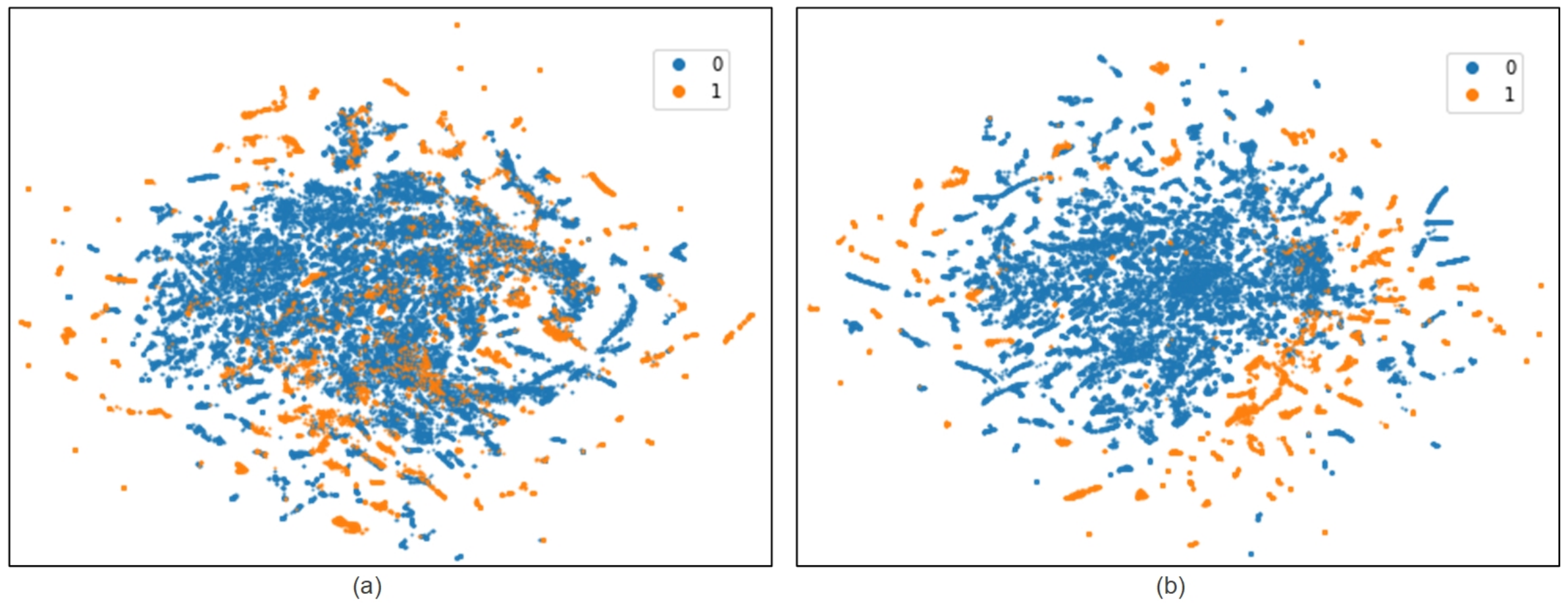
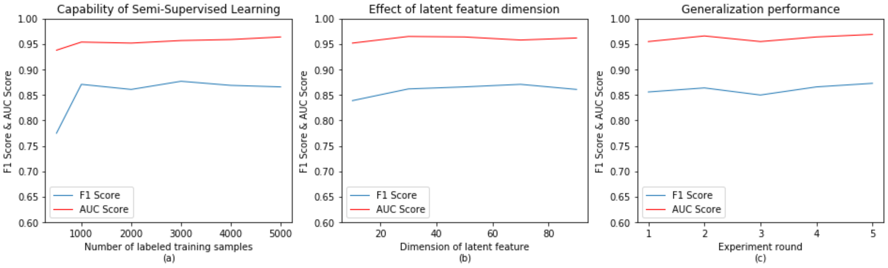
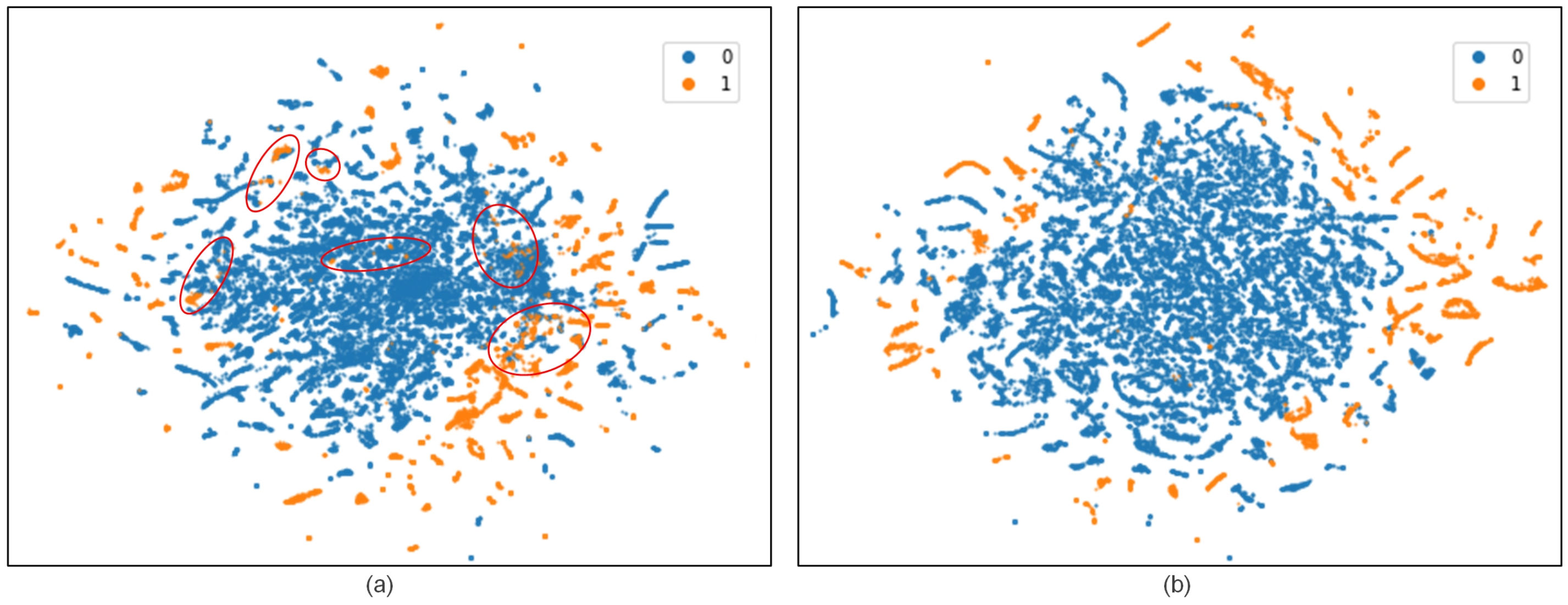
  • Capability of semi-supervised learning: As mentioned earlier, semi-supervised learning requires only a small number of labeled sample to complete the training of deep neural network and achieve ideal performance. Figure 7a provides the NTL detection effect of SSAE obtained with varying numbers of labeled samples. The results show that the SSAE can still obtain the F1 score of 0.775 and the AUC score of 0.938 with only 500 labeled samples. SSAE achieves the best results when the labeled sample reached 5000. Figure 8 further shows the feature learning ability of SSAE. By comparing two images, the overlapping regions of the features learned by SSAE in different categories become very small. It improves the linear separability of samples obviously.
  • Effect of latent feature dimension: The dimension of latent feature is a very important hyperparameter for SSAE. Figure 7b studied the effect of the dimension in the performance of SSAE. It can be seen from the results in Figure 7b, too small dimension will excessively cut down valid features, resulting in a decrease in the NTL detection performance. With the increase of the latent feature dimension, especially after more than 50, the effect will not continue to increase, but will decrease a little. The main reason is the latent features in larger dimension contains partial redundant information, which reduces its linear separability. By contrast, the best latent feature dimension is 50.
  • Generalization performance: In order to verify the generalization performance of SSAE, this paper launched the experiment with same parameters five times by randomly splitting the training set, validation set and testing set. The result of Figure 7c shows that the F1 score and the AUC score are between the ranges of [0.86, 0.883] and [0.965, 0.979], respectively. It is proved that SSAE has achieved remarkable generalization performance. In order to reflect the fairness of the comparison, the median results of SSAE were selected in subsequent subsections for comparison.
  • Convergence analysis: For semi-supervised learning, the number of epochs is a very important parameter to avoid underfitting and overfitting. In this paper, the epoch is defined by training all labeled samples rather than unlabeled samples. Too small or too large an epoch value will lead to underfitting or overfitting, respectively. Figure 9 provides losses and scores with the epoch from 1 to 100. Between 40 and 60 epochs, losses and scores are relatively flat and stable. Before 40 epochs and after 60 epochs, there are large fluctuations. Especially after 60 epochs, the training loss continued to fall, the validation loss began to rise. At same time, the AUC score and the F1 score both decreased slightly, and SSAE is over-fitting obviously. Moreover, in Figure 9, the AUC score and F1 score reach 0.9738 and 0.8763 at the 50th epoch, respectively. Therefore, the epoch value of all experiments in this paper is fixed at 50.

5.2.3. Comparison and Discussion

(1) Compared to Baselines
Table 4 and Figure 10 present the performance comparison of our approach and baselines. Overall, SSAE achieves the best results on all metrics. Benefit from the knowledge embedded sample model, SVM, KNN and XGBoost have also achieved good results, even using dimensionality reduction data as input features. Due to the stronger feature learning ability, MLP-3 and ResNet-20 is better than the above three methods. However, MLP-3 and ResNet-20 are supervised learning, and there can hardly avoid overfitting when labeled samples are extremely limited. In addition, the results of each of trial are very unstable. By using massive unlabeled samples and regularized losses, SSAE avoids overfitting successfully.
From Table 4, XGBoost obtained a good AUC score which close to the SSAE by selecting a very small decision threshold. Obviously, it will make the classifier be more sensitive, and lead to unstable. On the contrary, SSAE allows larger decision threshold without causing a significant drop in Precision and Recall. Refer to the results of SSAE presented in Table 4, Precision and Recall of SSAE outperform all baselines when the decision threshold is 0.5. It shows that SSAE separates normal and abnormal samples as much as possible. Hence, the classifier of SSAE will be more stable on varying scenarios.
(2) Comparison with other proposals
Table 5 shows a comparison between our method and the state-of-the-art approaches which report the AUC score and F1 score. It is worth mentioning that the AUC score or F1 score of state-of-the-art are referenced from their papers directly. Because our dataset cannot satisfy their requirements. For example, [35] needs observe meters as auxiliary data to help NTL detection. [3] requires GIS data, quality data and TECH data to achieve the best performance. [10,12] ask large number of labeled samples, and more than 1 year span of consumption data is [11]’s necessary condition.
Among these state-of-the-art approaches, [10,11,35] are based on artificial samples. The SMART attack model defined by [11] is the simplest situation because its fraud factor α t is dominated by a fixed parameter. Due to this reason, [11] achieves the AUC score of 0.99. However, the realistic NTL is more similar to the adaptive attack model(FDI5) defined by [10]. As the key factor of the FDI5 is changed randomly and timely, [10] achieves the F1 score of 0.83 and [35] achieves the AUC score of 0.851. Even though their performance are poor enough refer to [11], their results are more convincing.
On the other hand, [3,12] and the SSAE are validated on realistic NTL samples. The results in the Table 5 show that the SSAE has achieved a large lead on AUC score and F1 score. The knowledge embedded sample model and deep semi-supervised learning are key reasons. Although [12] is also based on deep neural networks, its model is designed on electricity consumption completely and without any domain knowledge, so that its AUC score is not ideal. To avoid the limitation of information on electricity consumption, [3] supplements various auxiliary or privacy data to achieve notable improvement. It undoubtedly increases the difficulty of data acquisition, especially some data refer to customers’ privacy. Our approach is a compromise solution which based on the SM data collected by the typical AMI system. It not only reduces the requirement of data types, but also protects customers’ privacy. Besides knowledge embedded sample model, the SSAE has stronger feature learning and NTL detection capabilities. Even if raw SM data, SSAE still obtains an AUC score of 0.907.

6. Conclusions

This paper provides a novel knowledge embedded sample model and deep semi-supervised learning algorithm to detect NTL by using SM data. We first analyzed the characteristic of realistic NTL, and design a knowledge embedded sample model refer to the principle of electricity measurement. Next, we proposed an autoencoder based semi-supervised learning model. To avoid overfitting, we designed a regularization module, loss and training algorithm. Overall, our scheme outperforms all baselines and state-of-the-art results. In future work, it is promising to explore a new sample model and deep neural networks to adapt to possible public datasets.

Author Contributions

Conceptualization, X.L. and Y.Z.; methodology, X.L., Y.Z. and Y.Y.; validation, X.L. and L.F.; resources, L.F.; writing—original draft preparation, X.L., Z.W. and Y.Y.; writing—review and editing, F.W.; supervision, Z.W.

Funding

This research was funded by State Grid Jiangsu Electric Power Co., Ltd. Science and Technology Project: Research on Key Technologies of Big Customers Abnormal Electricity Consumption Diagnosis Based on Deep Adversarial Learning (grant number: J2019048).

Conflicts of Interest

The authors declare no conflict of interest.

References

  1. Antmann, P. Reducing technical and non-technical losses in the power sector. In Background Paper for the WBG Energy Strategy; Technical Report; The World Bank: Washington, DC, USA, 2009. [Google Scholar]
  2. PR Newswire. World Loses $89.3 Billion to Electricity Theft Annually, $58.7 Billion in Emerging Markets. 2014. Available online: http://www.prnewswire.com/news-releases/world-loses-893-billion-to-electricity-theft-annually-587-billion-in-emerging-markets-300006515.html (accessed on 25 May 2019).
  3. Buzau, M.-M.; Tejedor-Aguilera, J.; Cruz-Romero, P.; Gomez-Exposito, A. Detection of Non-Technical Losses Using Smart Meter Data and Supervised Learning. IEEE Trans. Smart Grid 2019, 10, 2661–2670. [Google Scholar] [CrossRef]
  4. CEC. Monthly Statistics of China Power Industry. 2018. Available online: http://english.cec.org.cn/No.110.1737.htm (accessed on 25 May 2019).
  5. Messinis, G.M.; Hatziargyriou, N.D. Review of non-technical loss detection methods. Electr. Power Syst. Res. 2018, 158, 250–266. [Google Scholar] [CrossRef]
  6. Ahmad, T.; Chen, H.; Wang, J.; Guo, Y. Review of various modeling techniques for the detection of electricity theft in smart grid environment. Renew. Sustain. Energy Rev. 2018, 82, 2916–2933. [Google Scholar] [CrossRef]
  7. Wu, S.; Ji, C.; Sun, G.Q. A Clustering Algorithm Based on CUDA Technology for Massive Electric Power Load Curves. Electr. Power Eng. Teachnol. 2018, 37, 5–70. (In Chinese) [Google Scholar]
  8. Yang, X.; Zhang, X.; Lin, J.; Yu, W.; Zhao, P. A Gaussian-mixture model based detection scheme against data integrity attacks in the smart grid. In Proceedings of the 2016 25th International Conference on Computer Communication and Networks (ICCCN), Waikoloa, HI, USA, 1–4 August 2016; pp. 1–9. [Google Scholar]
  9. Glauner, P.; Meira, J.A.; Dolberg, L.; State, R.; Bettinger, F.; Rangoni, Y. Neighborhood features help detecting non-technical losses in big data sets. In Proceedings of the 2016 IEEE/ACM 3rd International Conference on Big Data Computing Applications and Technologies (BDCAT), Shanghai, China, 6–9 December 2016; pp. 253–261. [Google Scholar]
  10. Zanetti, M.; Jamhour, E.; Pellenz, M.; Penna, M.; Zambenedetti, V.; Chueiri, I. A Tunable Fraud Detection System for Advanced Metering Infrastructure Using Short-Lived Patterns. IEEE Trans. Smart Grid 2019, 10, 830–840. [Google Scholar] [CrossRef]
  11. Messinis, G.M.; Rigas, A.E.; Hatziargyriou, N.D. A Hybrid Method for Non-Technical Loss Detection in Smart Distribution Grids. IEEE Trans. Smart Grid 2019. [Google Scholar] [CrossRef]
  12. Zheng, Z.; Yang, Y.; Niu, X.; Dai, H.-N.; Zhou, Y. Wide and deep convolutional neural networks for electricity-theft detection to secure smart grids. IEEE Trans. Ind. Inform. 2018, 14, 1606–1615. [Google Scholar] [CrossRef]
  13. Jindal, A.; Dua, A.; Kaur, K.; Singh, M.; Kumar, N.; Mishra, S. Decision tree and SVM-based data analytics for theft detection in smart grid. IEEE Trans. Ind. Inform. 2016, 12, 1005–1016. [Google Scholar] [CrossRef]
  14. Coma-Puig, B.; Carmona, J.; Gavalda, R.; Alcoverro, S.; Martin, V. Fraud detection in energy consumption: A supervised approach. In Proceedings of the 2016 IEEE International Conference on Data Science and Advanced Analytics (DSAA), Montreal, QC, Canada, 17–19 October 2016; pp. 120–129. [Google Scholar]
  15. Nagi, J.; Yap, K.S.; Tiong, S.K.; Ahmed, S.K.; Mohamad, M. Nontechnical loss detection for metered customers in power utility using support vector machines. IEEE Trans. Power Deliv. 2009, 25, 1162–1171. [Google Scholar] [CrossRef]
  16. Jokar, P.; Arianpoo, N.; Leung, V.C. Electricity theft detection in AMI using customers’ consumption patterns. IEEE Trans. Smart Grid 2015, 7, 216–226. [Google Scholar] [CrossRef]
  17. Ramos, C.C.O.; de Souza, A.N.; Falcao, A.X.; Papa, J.P. New insights on nontechnical losses characterization through evolutionary-based feature selection. IEEE Trans. Power Deliv. 2011, 27, 140–146. [Google Scholar] [CrossRef]
  18. Monedero, I.; Biscarri, F.; León, C.; Guerrero, J.I.; Biscarri, J.; Millán, R. Detection of frauds and other non-technical losses in a power utility using Pearson coefficient, Bayesian networks and decision trees. Int. J. Electr. Power Energy Syst. 2012, 34, 90–98. [Google Scholar] [CrossRef]
  19. Krishna, V.B.; Weaver, G.A.; Sanders, W.H. PCA-based method for detecting integrity attacks on advanced metering infrastructure. In Proceedings of the 2015 12th International Conference on Quantitative Evaluation of Systems, Madrid, Spain, 1–3 September 2015; pp. 70–85. [Google Scholar]
  20. Júnior, L.A.P.; Ramos, C.C.O.; Rodrigues, D.; Pereira, D.R.; de Souza, A.N.; da Costa, K.A.P.; Papa, J.P. Unsupervised non-technical losses identification through optimum-path forest. Electr. Power Syst. Res. 2016, 140, 413–423. [Google Scholar] [CrossRef] [Green Version]
  21. Guerrero, J.I.; León, C.; Monedero, I.; Biscarri, F.; Biscarri, J. Improving knowledge-based systems with statistical techniques, text mining, and neural networks for non-technical loss detection. Knowl. Based Syst. 2014, 71, 376–388. [Google Scholar] [CrossRef]
  22. Wei, L.; Keogh, E. Semi-supervised time series classification. In Proceedings of the 12th ACM SIGKDD International Conference on Knowledge Discovery and Data Mining, Philadelphia, PA, USA, 20–23 August 2006; p. 748. [Google Scholar]
  23. Tacón, J.; Melgarejo, D.; Rodríguez, F.; Lecumberry, F.; Fernández, A. Semisupervised Approach to Non Technical Losses Detection. Phys. Lett. B 2014, 378, 698–705. [Google Scholar]
  24. Russakovsky, O.; Deng, J.; Su, H.; Krause, J.; Satheesh, S.; Ma, S.; Huang, Z.; Karpathy, A.; Khosla, A.; Bernstein, M.; et al. ImageNet Large Scale Visual Recognition Challenge. Int. J. Comput. Vis. (IJCV) 2015, 115, 211–252. [Google Scholar] [CrossRef] [Green Version]
  25. Deng, L.; Hinton, G.; Kingsbury, B. New types of deep neural network learning for speech recognition and related applications: An overview. In Proceedings of the 2013 IEEE International Conference on Acoustics, Speech and Signal Processing, Vancouver, BC, Canada, 26–31 May 2013; pp. 8599–8603. [Google Scholar]
  26. Wu, Y.; Schuster, M.; Chen, Z.; Le, Q.V.; Norouzi, M.; Macherey, W.; Krikun, M.; Cao, Y.; Gao, Q.; Macherey, K.; et al. Googles Neural Machine Translation System: Bridging the Gap between Human and Machine Translation. arXiv 2016, arXiv:1609.08144. [Google Scholar]
  27. Makhzani, A.; Shlens, J.; Jaitly, N.; Goodfellow, I.; Frey, B. Adversarial autoencoders. arXiv 2015, arXiv:1511.05644. [Google Scholar]
  28. Laine, S.; Aila, T. Temporal Ensembling for Semi-Supervised Learning. arXiv 2017, arXiv:1610.02242. [Google Scholar]
  29. Luo, Y.; Zhu, J.; Li, M.; Ren, Y.; Zhang, B. Smooth Neighbors on Teacher Graphs for Semi-Supervised Learning. In Proceedings of the IEEE/CVF Conference on Computer Vision and Pattern Recognition, Salt Lake City, UT, USA, 18–22 June 2018; pp. 8896–8905. [Google Scholar]
  30. Wang, R.C. Influence of Distribution Network Three-phase Unbalanceon Line Loss Increase Rate and Voltage Offset. Electr. Power Eng. Teachnol. 2017, 36, 131–136. (In Chinese) [Google Scholar]
  31. Maaten, L.V.D.; Hinton, G. Visualizing data using t-SNE. J. Mach. Learn. Res. 2008, 9, 2579–2605. [Google Scholar]
  32. Kingma, D.; Ba, J. Adam: A Method for Stochastic Optimization. arXiv 2014, arXiv:1412.6980. [Google Scholar]
  33. He, K.M.; Zhang, X.; Ren, S.; Sun, J. Deep residual learning for image recognition. In Proceedings of the IEEE Conference on Computer Vision and Pattern Recognition, Las Vegas, NV, USA, 26 June–1 July 2016; pp. 770–778. [Google Scholar]
  34. Pedregosa, F.; Varoquaux, G.; Gramfort, A.; Michel, V.; Thirion, B.; Grisel, O.; Blondel, M.; Prettenhofer, P.; Weiss, R.; Dubourg, V.; et al. Scikit-learn: Machine learning in Python. J. Mach. Learn. Res. 2011, 12, 2825–2830. [Google Scholar]
  35. Zheng, K.; Chen, Q.; Wang, Y.; Kang, C.; Xia, Q. A Novel Combined Data-Driven Approach for Electricity Theft Detection. IEEE Trans. Ind. Inf. 2018, 15, 1809–1819. [Google Scholar] [CrossRef]
  36. Coma-Puig, B.; Carmona, J. Bridging the Gap between Energy Consumption and Distribution through Non-Technical Loss Detection. Energies 2019, 12, 1748. [Google Scholar] [CrossRef]
Figure 1. Comparision of normal and Shunts by curves of voltages and currents.
Energies 12 03452 g001
Figure 2. Relationship between active power and power factor about phase inversion.
Energies 12 03452 g002
Figure 3. Structure of sample. (a) create samples based on shift window. (b) sample model embedded by knowledge.
Energies 12 03452 g003
Figure 4. t-SNE results of samples where 0 denotes normal samples plotted in blue, and 1 denotes NTL samples plotted in orange. (a) samples based on raw SM data. (b) samples based on raw SM data and electricity measurement knowledge.
Energies 12 03452 g004
Figure 5. Framework of Semi-Supervised Deep Neural Network.
Energies 12 03452 g005
Figure 6. The detail architecture of the SSAE modules.
Energies 12 03452 g006
Figure 7. Study the performance of SSAE according to varying proportion of labeled samples, latent size and experiment round. (a) Capability of semi-supervised learning against NTL. (b) Studying the effect of latent size to SSAE. (c) F1 score and AUC score on each round of experiment.
Energies 12 03452 g007
Figure 8. Comparison of t-SNE results of original samples and features learned by SSAE where 0 denotes normal samples plotted in blue, and 1 denotes NTL samples plotted in orange. (a) Original samples with embedding knowledge. (b) Latent features learned by SSAE.
Energies 12 03452 g008
Figure 9. Convergence analysis of SSAE.
Energies 12 03452 g009
Figure 10. The ROC curve and PR curve of SSAE and baselines.
Energies 12 03452 g010
Table 1. Electrical magnitudes of three-phase four-wire.
MagnitudeDescription
U A , U B , U C average voltage of each wire
I A , I B , I C average current of each wire
P t o t a l total active power
Q t o t a l total reactive power
f t o t a l total power factor
tstime-stamp
Table 2. Brief information of dataset.
Type of NTLNumber of CustomersNumber of Samples
Shunts of voltage141321
Shunts of current323609
Phase Shift161798
Phase Disorder252681
Phase Inversion586374
Normal customer31635,506
unlabeled4539500,000
Table 3. Comparison about sample embedded knowledge or not.
MethodsPrecisionRecallF1 ScoreAUC ScoreGeneral Accuracy
XGBoost + raw SM data0.9110.5380.6760.9170.905
XGBoost + knowledge embedded sample0.8460.7000.7660.9510.921
ResNet-20 + raw SM data0.9130.5780.7080.9160.909
ResNet-20 + knowledge embedded sample0.8910.7320.8040.9510.943
SSAE + raw SM data0.8820.5650.6890.9070.898
SSAE + knowledge embedded sample0.9440.8040.8660.9640.951
Table 4. NTL detection performance comparison (with knowledge).
MethodsPrecisionRecallF1 ScoreAUC ScoreGeneral Accuracy
SVM0.7260.6760.7000.9080.903
KNN0.8280.6270.7140.8660.907
XGBoost0.8460.7000.7660.9510.921
MLP-30.8440.7340.7850.9460.926
ResNet-200.8910.7320.8040.9510.934
SSAE0.9440.8040.8660.9640.951
Table 5. Comparison with the state-of-the-art.
MethodsAUC ScoreF1 ScoreNTL SampleDatasetResponse Time
[10]-0.83ArtificialImbalance3 weeks
[35]0.851-ArtificialImbalance1 month
[11]0.99-ArtificialBalance1 year
[3]0.91-RealImbalance90 days
[12]0.80-RealImbalance4 weeks
SSAE0.9640.866RealImbalance1 week

