Abstract
With the acceleration of industrialization, a large amount of energy consumption has brought tremendous pressure to the natural environment. In order to prevent environmental pollution and promote sustainable development, the environmental efficiency assessment as an effective way to provide decision-making basis has been given wide attention. This study measures the environmental efficiency of 30 provinces in China from 2006 to 2015 based on the Data Envelopment Analysis (DEA) environmental assessment radial model both under natural disposability and managerial disposability that considered the constant variable return to scale (RTS) and the damage to scale (DTS). In addition, the scale efficiency under the two kinds of disposability of China’s 30 provinces were also measured. We found that the environmental efficiencies of different provinces in China showed regional disparities. Provinces such as Beijing, Shanghai, and Guangdong had a good performance in unified environmental efficiency and scale efficiency both under natural disposability and managerial disposability. Generally speaking, the eastern regions always performed better than the central and western regions in unified environmental efficiency during the observed years. Therefore, policies should be established to distribute the resources in balance between the east, center, and west to further promote environmental efficiency.
1. Introduction
In recent years, remarkable achievements have been achieved in the development of China’s economy. According to the National Bureau of Statistics, the gross domestic product (GDP) increased from 367.87 billion RMB to 74,412.7 billion RMB during 1978 and 2016. However, the problems of “high energy consumption and high emissions” behind the economic rise should be recognized. Specifically, most of the regions place more emphasis on the growth of gross domestic product, while ignoring the resource consumption and environmental pollution. In addition, with the increasingly serious problem of haze in major cities, more and more people have begun to pay close attention to environmental governance and have realized the development model of “pollution first, then governance” is no longer suitable for the current requirement of sustainable development. Therefore, in order to promote sustainable development, the construction of an ecological civilization must be given more effort. Furthermore, the 19th National Congress of the Communist Party of China focused on the green development approach, brought up the ecological civilization as the “millennial target” for the everlasting development of the Chinese nation, and took the “harmony and coexistence of nature and human” as one of the basic guidelines of social development in the new era [1,2,3]. Hence, it is essential to provide suggestions for the formulation of national policies based on the evaluation and analysis of the environmental efficiency of all regions in order to promote sustainable development with coordination between economic growth and environmental protection in China.
A. Charnes and W. W. Cooper first proposed the method of Data Envelopment Analysis (DEA) in 1978 and the method first included undesirable outputs in 1989 [4]. Since then, more and more scholars have applied DEA methods to evaluate the efficiencies of energy and the environment in different fields and regions. A few examples of extensive research in the subject is given by Hu and Wang [5], who used the total-factor energy efficiency (TFEE) index to analyze the energy efficiency in 29 regions of China. Wei et al. [6] measured the efficiency of energy utilization in China’s steel industry and decomposed it into technology change and technological efficiency change. Zhou and Ang [7] first took carbon dioxide as a kind of undesirable output and then applied the DEA method to estimate the efficiency of 21 countries in the Organization for Economic Co-operation and Development (OECD). Yeh et al. [8] regarded sulfur dioxide as well as carbon dioxide as undesirable outputs to compare the efficiencies of energy utilization between the mainland and Taiwan. Yang and Pollitt [9] used the radial DEA method to analyze the environmental efficiencies in Chinese thermal power plants under different disposability. Fare et al. [10] took sulfur dioxide as well as nitrogen oxides as the undesirable outputs, and studied the interaction between the different pollutants and their shadow price as well as the conversion elasticity in American power plants via the directional distance function DEA model. Sueyoshi et al. [11] developed a new non-radial approach and used state-owned and private industries to carry out an empirical study, and then expanded it into a radial model [12]. Wang et al. [13] applied the RAM-DEA model to measure the integrated efficiency of energy and the environment under two kinds of disposability for China’s 30 regions from 2006 to 2010. Toshiyuki et al. [14] used the Malmquist index measurement to identify a frontier shift to improve the regional sustainable development level concerning 30 municipalities and provinces in China during 2003 and 2014. Wen et al. [15] proposed a cross efficiency approach by considering the game relationship among decision making units to measure and analyze the provincial efficiency of electric energy utilization in China’s 30 provinces from 2005 to 2014. Decai Tang et al. [16] evaluated the performance of environmental regulation during 2003 and 2013 by the slacks-based measure (SBM) undesirable model.
Reviewing the previous studies, it can be seen that most scholars have only focused on the performance analysis from a single perspective and have ignored the integrity of indictor selection in the process of evaluation with the DEA method. Therefore, the purpose of this paper was to combine the DEA environment assessment radial model with two kinds of strategies, the positive adaptation strategy and the negative adaptation strategy, which deal with the environmental regulations to study the environmental efficiency. Specifically, in the negative adaptive strategy, increased input can lead to a rise in undesirable output, while in the positive adaptation strategy, the increase would reduce the undesirable output by improving the technological level and optimizing management without any increased investment. In addition, the scale efficiency under managerial disposability and natural disposability was also taken into account in the analysis of environmental efficiency. Then, the proposed methods were applied to study China’s regional environmental efficiency from 2006 to 2015. Compared with the previous research, the undesirable outputs in this study included solid waste emissions, wastewater emissions, and waste gas emissions, which take full consideration of the environmental pollution problems caused by the production process.
The rest of this paper is organized as follows. Section 2 describes the DEA environment assessment radial model and the concepts of natural and managerial disposability. Moreover, the models of unified environmental efficiency with natural disposability under both the constant return to scale (RTS) and variable RTS are proposed. Then, the unified environmental efficiency under managerial disposability both under constant damage to scale (DTS) and variable DTS are introduced. In Section 3, we propose the indicators for the unified environmental efficiency. Subsequently, in the conditions of natural disposability and managerial disposability, the unified environmental efficiency and scale efficiency of 30 regions in China from 2006 to 2015 were evaluated and analyzed. Section 4 presents our conclusions.
2. The DEA Model
2.1. Variable Notations
Production factor notations:
- (1)
- , : vector including m inputs in the jth region.
- (2)
- , : vector including s desirable outputs in the jth region.
- (3)
- , : vector including h undesirable outputs in the jth region.
Aside from the above, there are other unknown variables that need to be measured:
- (4)
- : the known slack variable of the ith input.
- (5)
- : the known slack variable for the rth desirable output.
- (6)
- : the known slack variable for the fth undesirable output.
- (7)
- : vector of the unknown intensity or structure variable.
- (8)
- : the range for the jth input.
- (9)
- : the range for the rth desirable output.
- (10)
- : the range for the fth undesirable output.
- (11)
- : the minimum given by the DEA user.
- (12)
- : the invalid scores calculated by the DEA.
2.2. Two Strategies for Dealing with Environmental Regulation
Natural disposability: this concept indicates that a Decision Making Unit (DMU) is devoted to decrease the undesirable outputs by reducing the inputs. On the basis of reducing inputs and undesirable outputs, the DMU tries to increase the desirable outputs as far as possible. It can be regarded as a passive strategy to environmental regulation. In short, it refers to less inputs and less emissions.
Managerial disposability: this concept indicates that a DMU is devoted to increasing the inputs in order to increase the desirable outputs and reduce the undesirable outputs. Specifically, the DUM takes the changes of environmental regulation as a business opportunity to promote unified efficiency by using advanced environmental technologies and scientific management methods. It can be considered as a positive strategy toward environmental regulation. In a word, it is more investments and less emissions.
We point out that is the vector for inputs, is the desirable outputs vector, and is the vector for undesirable outputs. All of these vectors can be called production factors. Under the conditions of natural and managerial disposability, the unified production and pollution possibility sets are measured as follows:
where is a production possibility set under the variable RTS, while is under the variable DTS. The distinction between the two kinds of disposability is that the restrictive condition of under natural disposability is , while the restrictive condition of under managerial disposability is . The concepts are very intuitive because the efficient frontier of the desirable output is higher than all of the observed values, while the desirable output is to the contrary.
In addition, assume the sets of production and pollution possibility related to constant RTS and DTS by following:
There are two points to be noted about the four possible sets of production possibilities for the RTS and DTS under two types of disposal concept. (1) Under the condition of natural disposability, when evaluating the unified efficiency, the operating performance is the most important, followed by the environmental performance, while under management disposal, it is the opposite. (2) In terms of the sum of intensity variables, the requirements of RTS and DTS are different. The former contains the condition , while the latter does not. We can merge different RTS and DTS by defining the upper and lower bounds to dominate the size of .
Furthermore, it should be noted that in previous studies of DEA environmental efficiency, the total cost is generally assumed to be the minimum [12,17]. Usually, it is reasonable for an efficiency analysis to be based on this cost assumption, especially for countries in recession. However, it is not in line with the actual production situation. In general, the production cost is determined by the average cost (constant RTS and DTS) and the marginal cost (variable RTS and DTS), rather than the total cost [11,14,18]. Therefore, unlike the traditional DEA evaluation, this paper applied a DEA environmental assessment radial model that considered the DTS, RTS, and disposability under different conditions. This method can reflect the reality more truly and comprehensively to obtain more scientific and reasonable results, and provide a valuable reference for policy-making.
2.3. Unified Efficiency
The unified efficiency of DMU indicates that increasing inputs would produce desirable and undesirable outputs in the production process. A significant feature of the environmental evaluation with the DEA method is that each DMU is supposed to be comparable with others. The result of the comparation can be called the measurement of unified efficiency. According to Sueyoshi et al. [12], this paper applied a radial model to the DEA environmental evaluation as follows:
where represents an unrestricted and unknown invalid score, which is what dominates the distance between the observed vector and the efficiency frontier of the desirable and undesirable outputs. This paper assigned the minimum value ε as 0.0001 to reduce the influence of the slack variable and simplify the calculation. It is difficult to specify model (1) because is non-Archimedes infinitesimal. In order to overcome this, we assigned 0 to in model (1). However, in this case, some of the dual variables of the production factors will be 0, which will result in the production factor information in the model not being fully utilized. This is not reasonable as a result of the performance evaluation by the DEA method, so was the minimum in this paper.
Furthermore, model (1) exhibits nonlinear programming issues that cannot be solved directly. In this regard, there are two alternatives in which to solve this. On one hand, the first program is to introduce the nonlinear condition: as a constraint, and taking it as a nonlinear problem to solve. On the other hand, another program brings in the formulas: , , , , and , as constraints, then the original problem is transformed into a mixed integer programming problem to solve, where M represents an infinite number that needs to be defined before calculation. Through these two methods, the optimal solution or the unified efficiency of the Kth decision unit can be defined:
Therefore, the invalid scores as well as the slack variables can be calculated from the optimization of model (1).
2.4. Unified Efficiency under Natural Disposability
2.4.1. Unified Efficiency under the Conditions of Natural Disposability and Variable RTS (UENv)
The Kth unified efficiency under the conditions of natural disposability and variable RTS can be measured by the radial model as:
The UENV of the Kth DMU is measured by
Both the invalid scores and the slack variables can be calculated from the optimized model (Equation (3)). Additionally, the integrated efficiency is used to subtract the invalid scores from the population.
The dual programming of model (3) is as follows:
where vi, ui, wf represent the positive dual variables corresponding to the constraints in model (3), which are called the multiplier. The dual variable can be calculated based on the fourth formula of model (3). In terms of model (3) and model (5), there are three points that should be paid attention. The first is that the target value of model (3) is the optimal solution in model (5). Second, model (5) always produces positive dual variables, which are related to the scope of production factors. Therefore, we can make full use of the production factors in assessing model (3). Finally, each dual variable indicates that the change of the unit factor of production can lead to a change in the invalid scores accordingly.
2.4.2. Unified Efficiency under the Conditions of Natural Disposability and Constant RTS (UENc)
In order to satisfy the condition of constant RTS, the condition was taken out. The UENc can be defined as:
The optimal solution is obtained according to model (3) without the constraint .
2.4.3. Scale Efficiency under the Condition of Natural Disposability
Scale efficiency under the condition of natural disposability (SEN) represents the scale of operation managed when each DMU is under the condition of natural disposability, and is measured by: . When , is equal or less than the unified efficiency. The larger SEN score represents the better management scale in the condition of natural disposability.
Figure 1 intuitively describes the efficiency frontier under the two different conditions of RTS, and depicts a relationship between the desirable outputs on the vertical coordinate and the inputs on the horizontal coordinate. The straight line OG going through point B represents the efficiency frontier in the condition of constant RTS. The contour line (A-B-C-D-E) is an efficient frontier in the condition of variable RTS. Ω1 is a production possibility set for constant RTS. Ω1 Ω2 and Ω3 are three parts that constitute the variable production possible set of RTS. Decision unit F is invalid .

Figure 1.
Efficiency frontier of the desirable outputs under constant RTS and variable RTS.
2.5. Unified Efficiency under the Condition of Managerial Disposability
2.5.1. Unified Efficiency under Managerial Disposability and Variable DTS
Under the condition of managerial disposability, environmental performance is the most important, followed by the operating performance. Therefore, the unified efficiency under variable DTS of the Kth DMU is measured by:
Here, we changed the in model (3) into in model (7) to achieve the managerial disposability. The Kth DMU is formulated as follows:
According to the optimal solution of model (7), the invalid scores and all slack variables can be determined. The formula in the bracket refers to the invalid scores in the conditions of managerial disposability and DTS. Moreover, the unified efficiency can be determined by subtracting the invalid score from the whole. Then, the dual programming of model (7) is as follows:
where respectively represent the positive dual variable corresponding to the constraints in model (7), which are called the multiplier. The dual variable can be calculated based on the fourth formula in model (7). In addition, the target value of model (7) is the optimal solution in model (8).
The significant distinction between model (5) and model (8) is only in the objective function as the constraints of model (5) have and that of model (8) have . Therefore, the description of dual variables in model (5) is also applicable to model (8).
2.5.2. Integrated Efficiency under Managerial Disposability and Constant DTS (UEMc)
In order to meet the constant DTS, the condition is taken out. The UEMc can be defined as:
The optimal solution can be determined based on model (7) by eliminating the constraint .
2.5.3. Scale Efficiency in the Condition of Managerial Disposability
Scale efficiency in the condition of managerial disposability (SEM) represents how the scale of operation is managed under the condition of managerial disposability, and is measured by: . When , is equal or less than the unified efficiency. A larger SEM means that the management scale will be better under natural disposability.
Figure 2 intuitively describes the efficiency frontier under the two different conditions of DTS, and depicts the relationship between the undesirable outputs on the vertical coordinate and the inputs on the horizontal coordinate. The straight line OG going through point B represents the efficiency frontier in the condition of constant DTS. The contour line (A-B-C-D-E) is an efficient frontier under the variable DTS. In addition, Ω1 is a pollution possible set for constant DTS. Ω1, Ω2 and Ω3 are the three parts constituting the variable pollution possible set of DTS. The decision unit F is invalid and .

Figure 2.
Efficiency frontier of undesirable outputs under variable DTS and invariable DTS.
3. Empirical Studies
First, the variable selection of inputs as well as outputs is described in detail. Subsequently, the proposed model is applied to calculate the environmental efficiency of 30 provinces in China during 2006–2015, under different kinds of disposability. Finally, each of the provinces’ environmental efficiency are analyzed and discussed.
3.1. Variables and Data for Unified Efficiency
In DEA practices, the variable selection of input and output is a very important issue, where the purpose is to measure the efficiency of each DMU [19,20,21,22]. A relatively comprehensive obtained dataset can provide us with a more reasonable way to represent the evaluation problem. In addition, in order to identify the variable selection of input and output, we referenced and considered previous environmental efficiency studies [23,24,25,26]. According to these information sources, five input variables and one desirable output variable as well as three undesirable output variables were considered in this paper. Specifically, the five inputs included: (1) Labor, employed persons at year-end; (2) Capital, total fixed assets investment; (3) Water, total amount of water use; (4) Land, area of built districts; and (5) Energy, total energy consumption. The gross regional product (GRP) can be considered as the desirable output variable in the evaluation process. Furthermore, the three undesirable outputs included the total emission volume of waste gas; the total wastewater discharged; and the total solid waste generated.
The data of labor, capital, and land can be collected based on the China Statistical Yearbook. From the China City Statistical Yearbook, the data of the GRP can be collected. The total amount of water use, total emission volume of waste gas, total wastewater discharged, and solid waste generated data can all be obtained from the China Environmental Statistical Yearbook. Moreover, the total energy consumption data can be obtained through the China Energy Statistical Yearbook. However, considering the availability of data, Lhasa, Tibet, Hong Kong, Taiwan, and Macao were not included in the evaluation of environmental efficiency. Descriptive statistics of the relevant data are listed in Table 1.

Table 1.
Descriptive statistical data from 2006 to 2015.
3.2. Results and Discussion
According to the datasets we have discussed including the input variables (labor, capital, water, land and energy), desirable output variable (GDP), and undesirable output variables (waste gas, wastewater discharged and solid waste generated), the unified environmental efficiencies can be calculated. Subsequently, the results are shown in detail as follows.
3.2.1. Unified Environmental Efficiency under Natural Disposability
Table 2 shows the environmental efficiencies under the condition of natural disposability in 30 Chinese provinces from 2006 to 2015, where several conclusions can be drawn according to Table 2. First, in terms of environmental efficiency, Beijing, Tianjin, Shanghai, and Gansu performed well in the observed ten years. Their efficiency scores under natural disposability were equal to 1, whether they were under constant RTS and variable RTS. Hence, they could all be regarded as efficient during these ten years. Second, Zhejiang, Jiangsu, Shandong, Fujian, Guangdong, and Hainan also had good performance in unified environmental efficiency under natural disposability even though they were inefficient. Their environmental efficiency was close to 1 from 2006 to 2015. Finally, Shaanxi performed the worst. The unified environmental efficiency of Shaanxi was less than 0.3, which was the lowest among all of the provinces.
Table 2.
Unified environmental efficiency under natural disposability from 2006 to 2015.
Figure 3 summarizes the average environmental efficiency of each province under the conditions of natural disposability and constant RTS. According to Figure 3, it can be seen that there were four provinces, Beijing, Tianjin, Shanghai, and Gansu, whose average UENC was 1 in the past ten years that we studied. The efficient UENC shows that these provinces had the best performance both in GRP production and environmental protection under the condition of natural disposability. Therein, three of the four provinces were municipalities such as Beijing, Shanghai, and Tianjin. The four provincial governments did well in environmental pollution and showed good performance in environmental protection. Hence, they can be regarded as benchmarks for the unified environmental efficiency in other inefficient provinces.

Figure 3.
Average environmental efficiency under natural disposability and constant RTS.
In addition, it could be seen that there were five provinces, Jiangsu, Guangdong, Fujian, Zhejiang, and Hunan with the degree of average UENC over 0.8. Therein, Guangdong, Fujian, Zhejiang, and Jiangsu (as coastal provinces) are located in east China. Specifically, Guangdong Province has the most populous province, which accounts for 7.8% of China’s population. Since 1989, Guangdong’s GRP has ranked the first among all provincial-level divisions. As one of the richest provinces, Fujian, with its many industries, is situated on the southeast coast of China, adjacent to Zhejiang and Guangdong. After the reform and opening up, Fujian has attracted a lot of investment from overseas. The average UENC of Fujian was 0.907 in the observed ten years. In recent years, Zhejiang has shown great importance in prioritizing and encouraging entrepreneurship. Due to its unreasonable and inefficient demand for raw materials, cheap commodities produced by small enterprises cannot be transferred to technologically advanced industries. The average UENC was 0.9 during the observed ten years. The GRP of Jiangsu Province was the second highest among these provinces after Guangdong. The degree of average UENC of Jiangsu was 0.881 from 2006 to 2015. The degree of average UENC was 0.903 in 2006 and increased to 0.924 in 2010 with some small fluctuations. Hunan is a large province in the middle of China, and is located in the middle of the Yangtze River and south of Dongting Lake [27]. The pillar industry in Hunan Province mainly includes the construction industry, equipment manufacturing industry, non-ferrous metal industry, and cigarette manufacturing industry. The degree of average UENC was 0.851 in Hunan, and the four provinces were along the river or coastal areas.
There were also ten provinces such as Hainan, Shandong, Henan, Heilongjiang, Inner Mongolia, Hebei, Jiangxi, Jilin, Sichuan, and Hubei with the degree of UENC between 0.6 and 0.8. Hainan consists of various islands in the South China Sea and in recent years, the economic growth of Hainan has mainly depended on the development of the real estate industry. The average UENC of Hainan was 0.79 during the observed ten years. With its superior geographical position, Shandong has become one of the most populous and prosperous provinces in China, and the degree of average UENC was 0.762 during the observed ten years. In terms of Heilongjiang, private enterprises play an important role in promoting the economic growth of the whole province, and the unified environmental efficiency under natural disposability and constant RTS was 0.718. It should be noted that the two provinces of Hainan and Shandong are coastal provinces. They not only have a good performance economically, but also in the prevention of industrial pollution. However, the other provinces are located in the center of China. Compared with these two provinces, the rest showed poor performance in environmental protection and economic development.
As far as other provinces are concerned such as Chongqing, Guizhou, Guangxi, Shanxi, Yunnan, Xinjiang, Liaoning, Anhui, and Qinghai, the average UENC of these provinces were between 0.5 and 0.6. It can be seen that most of these provinces are located in western and central China. These provinces are densely populated, mostly labor-intensive industries, and the level of economic development is relatively backward. The extensive mode of economic development is also the main reason for the inefficiency of these provinces. Taking Shanxi as an example, because of the abundant resources of coal mines, the mining industry occupies a large proportion of its economic structure, but unreasonable mining methods also cause enormous environmental pollution. In addition, the local government focuses more on promoting economic development rather than environmental protection.
Finally, there are two provinces such as Ningxia and Shaanxi, ranked bottom in environmental protection with the degree of average UENC less than 0.5. They are located in western China, mainly in the highlands and mountains, with low population density and backward economy. Moreover, inadequate infrastructure in these provinces has also contributed to inefficiency to some extent. In particular, Shaanxi only had a degree of UENC at 0.03 on average.
3.2.2. Unified Environmental Efficiency under Managerial Disposability
Table 3 shows the environmental efficiency under the condition of managerial disposability in 30 Chinese provinces from 2006 to 2015 under both constant DTS and variable DTS. Some conclusions can be drawn from Table 3. First, Beijing, Hainan, and Xinjiang were efficient during the observed ten years. In other words, the degree of Unified environmental efficiency under managerial disposability (UEM) in Beijing, Hainan, and Xinjiang was maintained as 1 from 2006 to 2015. Second, Shaanxi, Gansu, Zhejiang, Jiangxi, Anhui, Henan, Shandong, Yunnan, Guizhou, and Ningxia had a decreasing UEMC during the studied ten years. Most of them are located in Central or Western China and indicates that the undeveloped regions are related to inefficient environmental efficiency. Due to the poor economic level, the governments have paid more attention to improving the economic situation, thus ignoring environmental protection. Finally, the degree of UEMC in Guangxi, Chongqing, and Sichuan increased from 2006 to 2015. These three provinces are located in the south of China. Taking Guangxi Province as an example, the UEMC of Guangxi was 0.556 in 2006 and increased to 0.73 in 2015 with some small fluctuations.
Table 3.
Unified environmental efficiency under managerial disposability from 2006 to 2015.
Figure 4 shows the average unified environmental efficiency under the conditions of both managerial disposability and constant DTS. From Figure 4, it can be seen that three provinces such as Beijing, Xinjiang and Hainan were all environmentally efficient during the observed ten years. The efficient UEMC indicates that these three provinces had the best performance in both GRP production and environmental protection for the ten years from 2006 to 2015, based on the assumption of managerial disposability. With the rapid development of Beijing, the government sector has paid more attention to the improvement of their environmental protection monitoring ability and therefore kept the degree of UEMC at the level of 1 since 2006. Hainan is a coastal province with a good economic performance and maintained their degree of UEMC at 1 from 2006 to 2015. Xinjiang is located in western China and a province that has large lands with a small population. Xinjiang showed good performance in environmental prevention, and can also be regarded as the benchmark for other inefficient western provinces in terms of improvement of environmental efficiency.

Figure 4.
Average environmental efficiency under managerial disposability and constant DTS.
In terms of the four provinces of Guangdong, Shanghai, Hunan, and Heilongjiang, though the four provinces were inefficient, they did well in the prevention of environmental pollution compared with the other provinces and the average UEMC was under 1 and over 0.8 in the observed ten years. Heilongjiang and Hunan are bordered with a river. Meanwhile, Guangdong and Shanghai are eastern coastal provinces. All of them have a good economic performance. Thus, the governments invested more resources in governing the industrial pollution, and the degree of UEMC was all over 0.8.
In addition, there were also nine provinces—Qinghai, Anhui, Yunnan, Guangxi, Shandong, Henan, Shanxi, Ningxia, and Liaoning—with a degree of average UEMC between 0.4 and 0.6. Among these provinces, Anhui, Henan, and Shanxi are in central China, while Qinghai and Ningxia lie to the west. Yunnan and Guangxi are located in south China. The economy of these provinces is undeveloped. However, Shandong and Liaoning are coastal provinces and Shandong has a good economic performance. The reason why the two provinces did worse in environmental efficiency is because the governments have attracted more and more investments to develop the economy. This kind of development style can cause heavy pressure on the ecological environment.
Hebei Province had a degree of average UEMC of 0.377, which ranked at the bottom of the 30 provinces. Hebei is an inland province and the pillar industry is the steel industry, which is a labor-intensive industry and produces a lot of pollution. Due to the underdeveloped economy and serious environmental pollution mainly brought about by the steel industry, the degree of UEMC of Hebei was very low from 2006 to 2015. This indicates that under the same conditions, the province will need much more input to maintain the same level of output.
3.2.3. Scale Efficiency
Table 4 summarizes the scale efficiency under the condition of natural disposability of the 30 provinces from 2006 to 2015. We noticed that Beijing, Tianjin, Shanghai, Guangdong, and Gansu had good performance in scale efficiency in the observed ten years. However, Shaanxi, Ningxia, and Qinghai had the lowest scale efficiency under natural disposability. The cluster map of average scale efficiency under the condition of natural disposability for all provinces from 2006 to 2015 is illustrated in Figure 5. There was a significant difference among these regions, which indicates that the government should be aware of the importance of resource distribution. In addition, the development of Shaanxi, Qinghai, Ningxia, and Liaoning should attract the attention of China’s government. It is apparent that the reform and opening up proposed by Xiaoping Deng has developed other provinces greatly, but not given enough importance to central and west China.
Table 4.
Scale efficiency under natural disposability from 2006 to 2015.
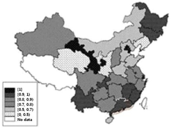
Figure 5.
Average scale efficiency under the natural disposability of 30 provinces in China (2006–2015).
Table 5 indicates the scale efficiency under the condition of the managerial disposability of these provinces during 2006 and 2015. According to Table 5, we found that Guangdong, Tianjin, Beijing, Heilongjiang, Hainan, and Xinjiang had good scores regarding scale efficiency during the ten years. The cluster map of average scale efficiency under the assumption of managerial disposability for these provinces is illustrated in Figure 6. The cluster map indicates that Liaoning, Hebei, Shanxi, Henan, Anhui, Shandong, and Qinghai performed the worst in the scale efficiency under managerial disposability.
Table 5.
Scale efficiency under managerial disposability from 2006 to 2015.

Figure 6.
Average scale efficiency under the managerial disposability of 30 provinces in China (2006–2015).
From Figure 5 to Figure 7 and Figure 8, we could observe the difference between the scale efficiency under natural disposability and managerial disposability as well as their changes over time during the observed period of all provinces. From a geographical perspective, the scale efficiency under managerial disposability was more balanced than that under natural disposability, and the SEN was lower than the SEM on average in 2006, while the SEN was higher than the SEM in 2015. According to Figure 6 and Figure 5, it can be found that regardless of the disposable conditions, the southern provinces were better than the northern provinces as a whole, in terms of environmental efficiency. In addition, Shaanxi and Qinghai had a large gap between the SEN and SEM, and the scale efficiencies under natural disposability were lower than that under managerial disposability. This indicates that these provinces need to put more effort into controlling the total input consumption and naturally decreasing the input utilization.

Figure 7.
The SEN and SEM of 30 Chinese provinces in 2006.

Figure 8.
The SEN and SEM of 30 Chinese provinces in 2015.
3.2.4. Discussion
Since the reform and opening up was raised by Deng Xiaoping in 1978, the eastern region in China, notably the municipality directly under the central government and Guangdong, has begun to focus more on economic growth. The policy, in which the government helps some people get rich first, then makes them help others, has caused economic unbalance to some degree. The government still attaches great attention to the development of the main cities, though the Chinese western development plan was formed in 2000.
In addition, the results of the analysis above indicate that the governments need to allocate more resources to the less-development regions and strengthen the development of small regions, especially those in northwest regions such as Shaanxi, Ningxia, Yinchuan, Qinghai, and Inner Mongolia through the utilization of effective and reasonable policies to promote economic growth and the development of environmental protection in the western region. Only when balanced regional development is realized can we achieve sustainable social development. On the other hand, the environment in major cities such as Beijing and Tianjin is becoming worse, with the occurrence of frequent smog weather. Governments are trying to improve the air condition in major cities, therefore, they need to enhance the management of energy enterprises and implement strict environmental protection policies in order to reduce the emissions of pollutants. Meanwhile, enterprises and individuals should also enhance their awareness of energy conservation and environmental protection in order to promote sustainable development.
4. Conclusions
Through the DEA environmental evaluation model, this paper studied the environmental performance under two different strategies: natural disposability and managerial disposability, which are responses to government environmental regulation. To be specific, with the panel datasets, this paper evaluated the environmental performance of 30 Chinese provinces from 2006 to 2015. In order to distinguish the economic growth and environmental protection among the different regions, the unified environmental efficiency under different conditions (RTS and DTS) and situations were measured thorough the DEA environmental assessment model.
Due to less industry and its coastal position, South China does a better job in protecting the environment than other regions. However, the governments in Northwest China, especially in Qinghai, Shaanxi, Ningxia, Inner Mongolia, etc., should pay attention to the distribution of resources (Capital, Education, Natural resources, Opportunities, etc.) to achieve balanced economic development. Through the diverse allocation of resources, the coordinated development of regional economic progress and environmental protection can be realized among the different regions. Meanwhile, the governments should practice stricter regulations on the industry, especially those of energy enterprises in major cities, to promote the improvement of environmental efficiency. In terms of achieving the objective of sustainable development, it is an indispensable step for China to carry out strategic transformation from economic growth to environmental protection.
Author Contributions
Conceptualization, X.Z.; Data curation, H.W.; Methodology, H.C.; Visualization and Validation, B.L.; Supervision, X.Z.; Writing—original draft, H.C.; Writing—review & editing, L.Q., X.Z. and B.L.
Funding
This work was funded by the National Natural Science Foundation of China (Grant No. 71871175), Shaanxi Province Innovative Talents Promotion Plan-Youth Science and Technology Nova Project (Grant No.2019KJXX-031), the China Postdoctoral Science Foundation Funded Project (Grant No. 2018M640188), and the Seed Foundation of Innovation Practice for Graduate Students at Xi’dian University. The authors are grateful to the support of these projects and all the research participants.
Conflicts of Interest
The authors declare no conflict of interest.
References
- Zhang, J.; Liu, Y.; Chang, Y.; Zhang, L. Industrial eco-efficiency in China: A provincial quantification using three-stage data envelopment analysis. J. Clean. Prod. 2017, 143, 238–249. [Google Scholar] [CrossRef]
- Lyu, K.; Bian, Y.; Yu, A. Environmental efficiency evaluation of industrial sector in China by incorporating learning effects. J. Clean. Prod. 2018, 172, 2464–2474. [Google Scholar] [CrossRef]
- Chen, L.; Jia, G. Environmental efficiency analysis of China’s regional industry: A data envelopment analysis (DEA) based approach. J. Clean. Prod. 2017, 14, 846–853. [Google Scholar] [CrossRef]
- Färe, R.; Grosskopf, S.; Lovell, C.K.; Pasurka, C. Multilateral productivity comparisons when some outputs are undesirable: A nonparametric approach. Rev. Econ. Stat. 1989, 71, 90–98. [Google Scholar] [CrossRef]
- Hu, J.L.; Wang, S.C. Total-factor energy efficiency of regions in China. Energy Policy 2006, 34, 3206–3217. [Google Scholar] [CrossRef]
- Wei, Y.M.; Liao, H.; Fan, Y. An empirical analysis of energy efficiency in China’s iron and steel sector. Energy 2007, 32, 2262–2270. [Google Scholar] [CrossRef]
- Zhou, P.; Ang, B.W. Linear programming models for measuring economy-wide energy efficiency performance. Energy Policy 2008, 36, 2911–2916. [Google Scholar] [CrossRef]
- Yeh, T.L.; Chen, T.Y.; Lai, P.Y. A comparative study of energy utilization efficiency between Taiwan and China. Energy Policy 2010, 38, 2386–2394. [Google Scholar] [CrossRef]
- Yang, H.; Pollitt, M. The necessity of distinguishing weak and strong disposability among undesirable outputs in DEA: Environmental performance of Chinese coalfired power plants. Energy Policy 2010, 38, 4440–4444. [Google Scholar] [CrossRef]
- Färe, R.; Grosskopf, S.; Pasurka, C.A., Jr.; Weber, W.L. Substitutability among undesirable outputs. Appl. Econ. 2018, 44, 39–47. [Google Scholar]
- Sueyoshi, T.; Goto, M. Data envelopment analysis for environmental assessment: Comparison between public and private ownership in petroleum industry. Eur. J. Oper. Res. 2012, 216, 668–678. [Google Scholar] [CrossRef]
- Sueyoshi, T.; Goto, M. Environmental assessment by DEA radial measurement: U.S. coal-fired power plants in ISO (independent system operator) and RTO (regional transmission organization). Energy Econ. 2012, 34, 663–676. [Google Scholar] [CrossRef]
- Wang, K.; Lu, B.; Wei, Y.M. China’s regional energy and environmental efficiency: A Range-Adjusted Measure based analysis. Appl. Energy 2013, 112, 1403–1415. [Google Scholar] [CrossRef]
- Sueyoshi, T.; Goto, M.; Wang, D. Malmquist index measurement for sustainability enhancement in Chinese municipalities and provinces. Energy Econ. 2017, 67, 554–571. [Google Scholar] [CrossRef]
- Chen, W.; Zhou, K.; Yang, S. Evaluation of China’s electric energy efficiency under environmental constraints: A DEA cross efficiency model based on game relationship. J. Clean. Prod. 2017, 164, 38–44. [Google Scholar] [CrossRef]
- Tang, D.; Tang, J.; Xiao, Z.; Ma, T.; Bethel, B.J. Environmental regulation efficiency and total factor productivity—Effect analysis based on Chinese data from 2003 to 2013. Ecol. Indic. 2017, 73, 312–318. [Google Scholar] [CrossRef]
- Sueyoshi, T.; Yuan, Y.; Goto, M. A literature study for DEA applied to energy and environment. Energy Econ. 2017, 62, 104–124. [Google Scholar] [CrossRef]
- Sueyoshi, T.; Yuan, Y. Return to damage under undesirable congestion and damages to return under desirable congestion measured by DEA environmental assessment with multiplier restriction: Economic and energy planning for social sustainability in China. Energy Econ. 2016, 56, 288–309. [Google Scholar] [CrossRef]
- Zeng, S.; Xu, Y.; Wang, L.; Chen, J.; Li, Q. Forecasting the allocative efficiency of carbon emission allowance financial assets in China at the provincial level in 2020. Energies 2016, 9, 329. [Google Scholar] [CrossRef]
- Mardani, A.; Streimikiene, D.; Balezentis, T.; Saman, M.; Nor, K.; Khoshnava, S. Data envelopment analysis in energy and environmental economics: An overview of the state-of-the-art and recent development trends. Energies 2018, 11, 2002. [Google Scholar] [CrossRef]
- Caunii, A.; Negrea, A.; Pentea, M.; Samfira, I.; Motoc, M.; Butnariu, M. Mobility of heavy metals from soil in the two species of the aromatic plants. Rev. Chim. 2015, 66, 382–386. [Google Scholar]
- Dong, X.H.; Hu, Y.L.; Li, W.X. An international comparisons and historical analysis on China’s environmental governance efficiency based on the bode of DEA. Stud. Sci. Sci. 2008, 6, 105–114. (In Chinese) [Google Scholar]
- Bian, Y.; Yang, F. Resource and environment efficiency analysis of provinces in China: A DEA approach based on Shannon’s entropy. Energy Policy 2010, 38, 1909–1917. [Google Scholar] [CrossRef]
- Wang, K.; Yu, S.; Zhang, W. China’s regional energy and environmental efficiency: A DEA window analysis based dynamic evaluation. Math. Comput. Model. 2013, 58, 1117–1127. [Google Scholar] [CrossRef]
- Yang, Z.; Wang, D.; Du, T.; Zhang, A.; Zhou, Y. Total-Factor energy efficiency in China’s agricultural sector: Trends, disparities and potentials. Energies 2018, 11, 853. [Google Scholar] [CrossRef]
- Chen, X.; Gong, Z. DEA Efficiency of energy consumption in China’s manufacturing sectors with environmental regulation policy constraints. Sustainability 2017, 9, 210. [Google Scholar] [CrossRef]
- Chang, Y.T.; Zhang, N.; Danao, D.; Zhang, N. Environmental efficiency analysis of transportation system in China: A non-radial DEA approach. Energy Policy 2013, 58, 277–283. [Google Scholar] [CrossRef]
© 2019 by the authors. Licensee MDPI, Basel, Switzerland. This article is an open access article distributed under the terms and conditions of the Creative Commons Attribution (CC BY) license (http://creativecommons.org/licenses/by/4.0/).