Parsing the Effects of Wind and Solar Generation on the German Electricity Trade Surplus

Abstract

Germany has experienced rapid growth in its renewable electricity generation capacity in the past fifteen years. This development has been accompanied by a drop in wholesale electricity prices and significant net export surpluses. This situation has given rise to discussions in policy circles concerning the drivers behind these dynamics. The paper at hand empirically analyzes historical cross-border commercial flows (CBCF) of electricity from Germany by applying a Ridge Regression model to parse the effects of the growing shares of renewable energy capacity on the commercial electricity exchange between 2012 and 2016. In case of PV, the fraction of PV generation (marginal effect of PV on export) that is exported correlates positively with the level of PV generation. However, the marginal effect of wind on export is negatively correlated with the level of wind generation. A possible explanation for this finding as it relates to wind feed-in could involve the high degree to which the grid is constrained at times of high wind penetration.

1. Introduction and Background

Germany is currently in the midst of implementing its Energiewende (energy transition), steadily increasing the share of variable renewable energy sources (VRE) as a percentage of its electricity production over the past decade. There has been a sharp increase in the installed capacity of VRE sources, most prominently onshore wind energy (from 18.4 GW in 2005 to 50.3 GW in 2017) and PV (from 10.57 GW in 2005 to 43.3 GW in 2017). Offshore wind energy has likewise increased steadily since 2012, from under 300 MW to ca. 5.3 GW by the end of 2017 [1]. The increasing volumes of VRE production has not only had a significant impact at the grid level but has also had a bearing on the development of wholesale prices. At the same time, the growing share of renewable power production has been accompanied by an increasing volume of electricity exports.

Physical net exports rose sharply from 2010 to 2016 (from ca. 18 TWh to over 50 TWh). In commercial terms, absolute levels of exports increased from 2012 to 2015 to a level in excess of EUR 2 billion. In 2016, the trade balance fell slightly to around EUR 1.75 billion. Furthermore, Figure 1 highlights the distribution of the net position across the year, indicating higher export levels in winter as opposed to summer months. The trends observed raise initial questions as to the impact of seasonal weather and load patterns on Germany’s net position while the dip in the surplus in 2016 poses questions as to the transitory nature of the drop.

These trends have drawn a great deal of attention with regard to their causal relationships as relates to physical impacts on the transnational grid infrastructure as well as welfare effects in the respective countries. In particular, the effect of growing shares of VRE in the German electricity system and their influence on export volumes has been discussed in policy circles with questions being raised about the extent to which intermittent renewable generation is driving the growth of the net export surplus or if the root of the export frequency stems from the operational inflexibilites of conventional, baseload power plants [3].

Concurrent to the development in the shares of VRE in Germany, the European electricity markets have been undergoing a continuous process of integration. Starting with the markets in the Central Western European (CWE) region (covering Benelux, France and Germany), which were coupled in 2010, price coupling was instituted in 2014 for the countries of Northwestern Europe (NWE), covering the CWE region, Great Britain as well as the Nordic and Baltic states. With the inclusion of Spain and Portugal and the coupling of Italy with France, Austria and Slovenia, the currently coupled market area has expanded to cover 19 countries, representing ca. 85% of European electricity consumption. This region carries the designation of the Multi-Regional Coupling. The implicit allocation of interconnection capacity via market coupling has facilitated a more efficient use of cross-border interconnection capacity. In mid-2015, the capacity allocation mechanism referred to as Flow Based Market Coupling (FBMC) was introduced in the CWE region to enhance the efficiency of calculating cross-border capacities by improving the representation of the physics of the grid while maintaining a zonal approximation of the commercial exchange between countries [4].

In connection with these developments, various analyses have examined the extent to which market integration has materialized, evaluating the instance of convergence between national power prices across the coupled markets. Furthermore, the effect of VRE on price convergence in the context of market coupling has also been looked at for selected countries [5].

Against this backdrop, the following analysis provides a detailed consideration of the causes of the large German electricity trade surplus. In particular, the research questions include analyzing the effect of VRE on supply and price and in turn cross-border trade and, subsequently, quantifying the elasticity of Germany’s net position with respect to wind and solar generation. Tying in the European context, the influence of the introduction of FBMC is also evaluated.

The remainder of the paper is structured as follows. After a discussion of the extant literature is conducted in Section 2, Section 3 introduces the theoretical framework. The data and methodological approach used in the analysis are presented in Section 4. In Section 5, the results of the empirical analysis are derived and discussed. The paper concludes with a recapitulation of the key takeaways of the analysis with a brief outlook towards areas for further research in Section 7.

2. Review of Empirical Findings on the Effects of VRE Generation in the Context of Market Coupling

The paper at hand addresses the confluence of two streams of literature: The impact of VRE feed-in on domestic electricity prices as well as the fundamentals of cross-border electricity trade and integration of European electricity markets. The interplay between the feed-in of VRE and domestic electricity price movements is the subject of a growing amount of empirical research. As it relates to the effect of VRE on domestic electricity prices, an ample amount of research has examined the influence of solar and wind feed-in on the absolute price level as well as its volatility. Examples that consider the effects in the former German–Austrian market zone include [6,7,8,9,10,11,12,13]. While analyzing data from different time periods using both econometric and model-based simulations, the overarching findings conclude that on account of the merit-order effect, renewable feed-in negatively impacts wholesale electricity prices. A comprehensive overview of the research on the impact of VRE on electricity prices with a supplemental empirical evaluation using a multi-variant regression model is provided in [14]. The analysis indicates that the price effect of generation from wind and solar energy sources is similar. For the former German-Austrian market zone, the price on the day-ahead market fell by 1 EUR/MWh for each additional GWh of expected generation from VRE. More recently, reference [15] confirm that the growing shares of wind generation and photovoltaic feed-in drove the sharp drop in electricity prices between 2012 and 2015. The authors also point out that wind has a stable impact throughout the day while PV has the most pronounced influence at midday.

In a European context, the issue of market integration and cross-border commercial flows has also also been examined in great detail. As a top policy priority, starting in 2003 the European Union has increasingly sought to enact measures enhancing cross-border electricity trade to increase welfare by improving security of supply and stimulating competition. These prospective benefits have been detailed and quantified in, e.g., [16,17]. Pertaining to evaluating the degree of transnational integration, early publications including, e.g., [18,19], demonstrate empirically that price convergence at spot markets between European member states had only partially been achieved while identifying persisting inadequacies in the institutional framework relating to auctioning interconnector capacities. In [20], the authors find evidence of market integration between French, German, British, Dutch and Spanish electricity markets increasing over time with the proximity of neighboring countries having a muted impact on the magnitude of integration. More recent publications have provided mixed conclusions on the state of market integration. Analyzing prices on 13 European electricity spot markets during the period 2007–2012, in [21], the authors observe increased price convergence in the wake of the implementation of the European Commission’s Third Energy Package. Examining an extended sample of spot prices from 2000 to 2013 in nine European electricity spot markets as well as month-ahead prices in four markets between 2007 and 2012, evidence of convergence between forward prices while observing a persisting divergence in spot prices across the markets has been observed [22]. In [23], an empirical investigation of price convergence of day-ahead prices across 25 European markets between 2010 and 2015 was carried out. They conclude that after an initial uptake in market integration between 2010 and 2012, a subsequent decline is observed, occurring at the same time market coupling was being expanded.

More in line with the research focus of the paper at hand, with respect to the effect of VRE on the commercial cross-border exchange [5] demonstrate, based on a sample of hourly French and German day-ahead prices from 2009 to 2013, that VRE production in Germany has significantly contributed to price divergences between the two markets. The panel regression performed indicates that large volumes of solar and wind energy generation are being exported to neighboring countries leading to incidences of congested interconnections and diverging day-ahead prices. While the introduction of market coupling in 2011 initially mitigated the effects, the analysis establishes that growing shares of VRE have displaced positive efficiency gains. A similar analysis with a stronger emphasis on volatility spillovers between the two markets has been carried out in [24]. Based on data from 2012 to 2015, the authors show that variable wind energy generation in Germany considerably impacts both German and French electricity prices. They also demonstrate that market coupling has a mitigating effect on the price variance between the markets, but note that the coupling of the markets has increased the transmission of price volatility caused by intermittent wind generation. Focusing on the impact of wind power generation on cross-border power transmission, the authors of [25] employ principal component analysis in combination with a subsequent regression model and demonstrate that wind power forecasts and spot price movements in Germany significantly affect cross-border power flows in Europe.

To the authors’ knowledge, apart from [26] there have been no other publications that directly address disaggregating the factors influencing the increase in German electricity exports in recent years. In [26], the authors provide a brief qualitative discussion of the causes of the large commercial electricity trade surplus in 2013. They put forth the observation that analyzing the net trade balance in the context of the hourly power plant dispatch, there is a strong indication that a significant amount of electricity was exported at times when solar and wind feed-in was at its highest. This observation is grounded in basic economic trade theory. Additionally, the authors point to the oversupply of generation capacity and a comparatively efficient domestic power plant fleet as causes for the trade surplus. Due to the nature of the support system for VRE in Germany, it is noted that the electricity exports can be considered an externality entailing distributional effects that should be evaluated.

As can be gleaned from the review above, the extant literature addresses various aspects of cross-border commercial exchange, however, empirically parsing the extent to which VRE generation is contributing to the Germany export surplus and evaluating their implications for the integration of wind and solar feed-in has yet to be specifically addressed. Thus, the analysis at hand extends previous work by addressing the question as to what effect the generation from VRE sources had on the price elasticity of German electricity exports between 2012 and 2016.

3. Theoretical Framework: Trade Theory in Electricity Markets

To support the following analysis, a brief overview of trade theory in the context of power markets is provided. Considering two connected markets trading in a homogeneous good like electricity with unrestricted cross-border transmission capacities, the price disparities in the two markets converge to an equilibrium price.

In Figure 2, the prices in the market with the higher domestic price $P_A$ drops to the equilibrium market price $P_{A+B}$. While the domestic price in the market with the initially lower price level $P_B$ rises to the equilibrium price. Electricity is exported ($Exp$) from region B to region A.

Assuming that region B introduces substantial shares of VRE (Figure 3), the supply function of the region shifts to the right as VRE are bid into the market clearing at negligible marginal costs. This causes the price in the region to fall to $P_{B_{res}}$ (without considering cross-border exchanges). However, the prices in region B increase as a result of the exported volumes. Since there is no incidence of congestion, the prices converge to $P_{A+B_{res}}$, which is lower than the price level in the previous case ($P_{A+B}$). The prices in region A fall further than in the previous case by $\Delta P_A$. The amount of exports from region B to region A increases by $\Delta Export$.

These two theoretical examples indicate that cross-border trade leads to increases in prices in the exporting country and a decrease in prices in the importing country. The increase in VRE generation results in a price decline in both markets. Furthermore, it should be noted that the increase in VRE also leads to an increase in exports at lower prices.

While this theoretical framework explains the fundamentals of market operation, it is important to recognize that the framework cannot explain all aspects of market operation. Relevant to the paper at hand is the aspect of integrating of VRE into the market. Here, the theoretical framework proves limited as it fails to take into account the flexibility of the system (the framework analysis provides merely a snapshot of the market operation), interplay between different generation sources and the prevailing network conditions.

In the following section, the empirical validity of these comparative statistics are explored further using historical data for VRE generation, which builds the basis for the subsequent empirical estimation conducted.

4. Data Description and Exploratory Analysis

The primary dataset used in the analysis was provided by Agora Energiewende [2]. The data is based on various sources and was cleaned and processed by Agora Energiewende. In addition to this dataset, the national generation capacity data was sourced from Open Power System Data [27].

Table 1. Data sources for generation and price data.

Variable	Source	Year
Cross-border commercial flows	Agora Energiewende	2012–2016
Generation (technology-specific)	Agora Energiewende	2012–2016
Load (Germany)	Agora Energiewende	2012–2016
Day Ahead Spot Prices (Germany)	Agora Energiewende	2012–2016
National generation capacity (Germany)	Open Power System Data	2012–2016

provides and overview of the data used in the analysis.

Table A1. Descriptive statistics of input data.

	Count	Mean	Std.Dev	Min	Max
Net Position (MW)	43,848	4779	3594	−7449	16,941
Generation (MW)	43,848	57,437	9871	12,170	91,233
Day Ahead Price (EUR)	43,848	35	16	−222	210
Load (MW)	43,848	63,727	9395	9749	91,340
Capacity Onshore (MW)	43,848	34,828	5499	26,965	45,438
Capacity Offshore (MW)	43,848	1485	1410	188	4131
Capacity PV (MW)	43,848	35,633	3823	25,969	40,294
Wind Generation (MWh)	43,848	7205	6336	0	33,713
PV Generation (MWh)	43,848	3863	5998	0	28,829

in Appendix A provides descriptive statistics on the data used in the analysis.

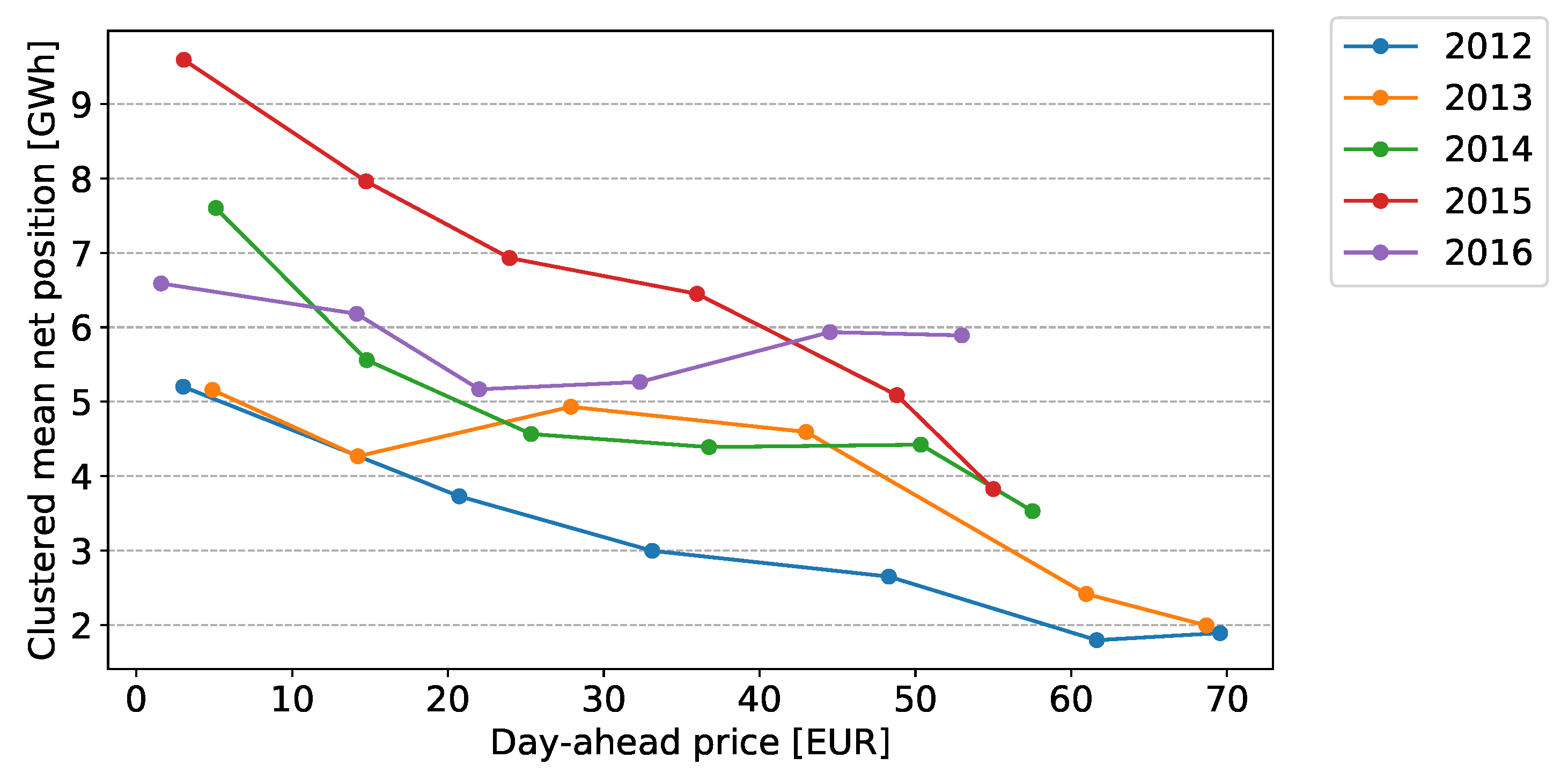
Figure 4 depicts the net export of electricity for Germany as a function of day-ahead prices. To observe the aggregate impact of prices on export, the data was clustered in unevenly sized groups. The clusters are grouped together based on the level of day-ahead prices within a year. The bins represent the following quantiles of day-ahead prices: [0–5], [5–10], [10–40], [40–90], [90–95], [95–100]. While some year-specific characteristics can be observed, at an aggregate level, the graph shows an inverse relationship between the commercial exports and electricity prices. The figure also highlights the increasing frequency of net exports at low day-ahead market price from 2012–2015 with a slight deviation in 2016.

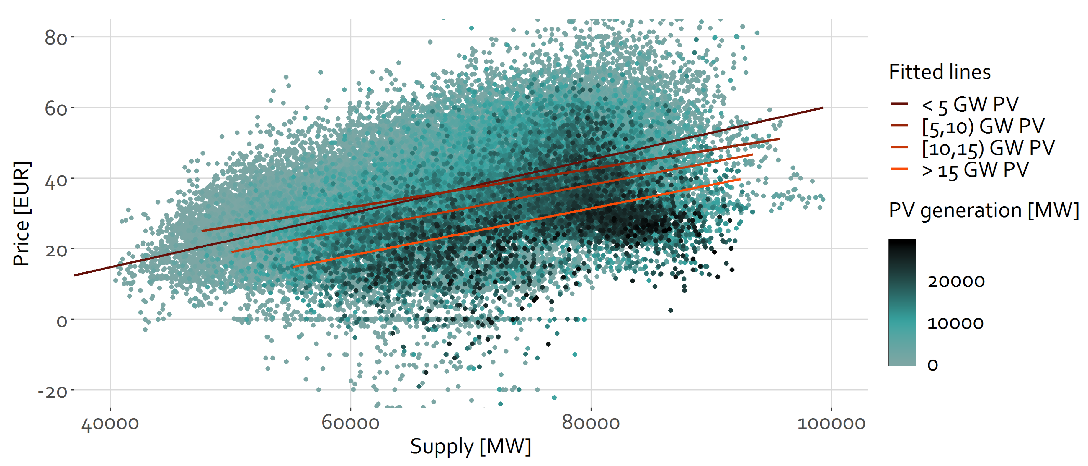
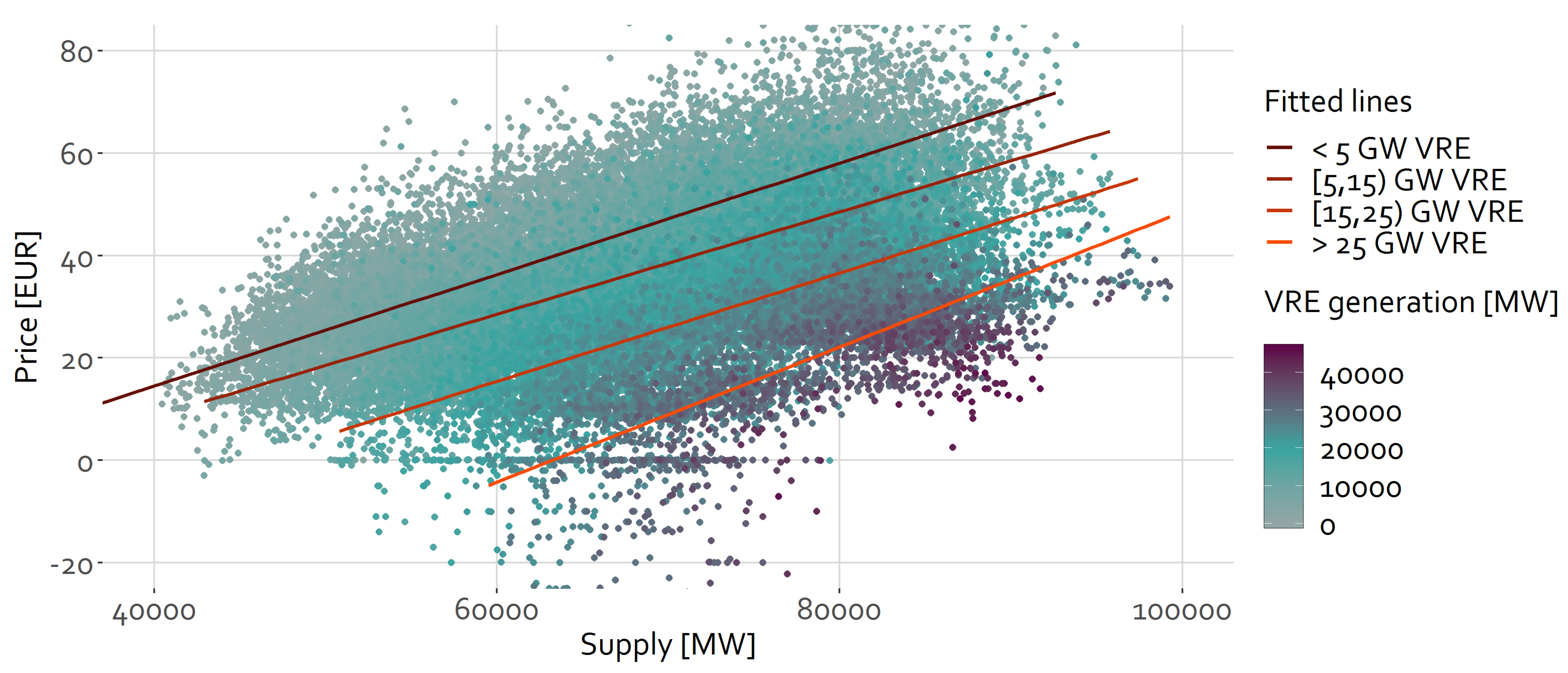
Figure 5, Figure 6 and Figure 7 depict the relationship between total power generation and the price for electricity in Germany for the years 2012 to 2016. The figures share the same data points (all available observations, cf. Table A1), but additionally display different levels of PV, wind and total VRE generation, respectively.

The positive correlation between total supply and price can be observed from the scatter plots. Also, in all three figures, higher renewable generation levels tend to concentrate in the lower part of the data spectrum, which means that they coincide with lower price levels. Very high PV generation is also more concentrated on the right side, additionally coinciding with higher levels of overall supply. Naturally, this is due to PV’s high correlation with load due to diurnal patterns. In addition, periods of very high PV generation are characterized by low to medium prices as opposed to times with high wind or overall VRE generation, which exhibit low to very low prices.

Furthermore, Figure 5, Figure 6 and Figure 7 display four lines of best fit. These are based on the correlation between price and supply for four different subsets. For PV and wind, the subsets contain generation levels from 0–5 GW, 5–10 GW, 10–15 GW and >15 GW. For VRE, the subsets contain generation levels from 0–5 GW, 5–15 GW, 15–25 GW and >25 GW. The increasing generation levels of the categories correspond with brighter lines (dark red for the lowest generation level category to orange for the highest). In all three figures a downward trend in the lines is observable corresponding with the increasing renewable generation levels of the subsets. This effect is more substantial for wind energy than for PV generation. The combined effect of both technologies is the largest.

In general, the exploratory analysis supports the theoretical assumption that renewable generation causes a downward shift in the supply curve, thereby leading to greater export volumes and a lower import price for the importing country.

While this exploratory analysis provides a fundamental understanding of the market dynamics at play and the impact of VRE generation on exports, a more sophisticated regression analysis is required to parse the effects of PV and wind generation on the price elasticity of German CBCF as well as the impacts of the introduction of FBMC on commercial export volumes.

5. Methodological Approach

To further analyze if the positive effect on exports is larger for wind energy than for PV, as suggested by the exploratory analysis, a linear regression analysis model is developed.

The linear regression model is of the following form:

$$\begin{array}{cc}\hfill N{P}_t=& {\mathsf{\beta }}_0+{\mathsf{\beta }}_{1}F{B}_t+{\mathsf{\beta }}_{2}Loa{d}_t+{\mathsf{\beta }}_{3}Pric{e}_t+{\mathsf{\beta }}_{4}Win{d}_t+{\mathsf{\beta }}_{5}P{V}_t+\hfill \\ \hfill & {\mathsf{\beta }}_{6}Ca{p}_{\mathrm{Onshore},t}+{\mathsf{\beta }}_{7}Ca{p}_{\mathrm{Offshore},t}+{\mathsf{\beta }}_{8}Ca{p}_{\mathrm{PV},t}\hfill \\ \hfill & \mathbf{H}\mathsf{\eta }+\mathbf{M}\mathsf{\mu }+\mathbf{Y}\mathsf{\upsilon }+\mathbf{X}\mathsf{\xi }+{\mathsf{ϵ}}_t\hfill \end{array}$$

(1)

The net position (balance of export and imports) of Germany represents the dependent variable in Equation (1). By using net position (not just export) we capture, to some extent, the response of the neighbouring countries. Aggregated load, the day-ahead price, wind and PV generation along with the installed capacities for PV, wind onshore and wind offshore serve as explanatory variables. Additionally, in order to capture the effect of FBMC, a flow-based dummy variable is included, which is set to 0 for all dates up to May 19, 2015 and set to 1 for all dates thereafter. Conventional generation is not represented in the model because its inclusion would almost fully explain the dependent variable, leading to near perfect multicollinearity (in addition to generation and load, the net position comprises losses, however, load and generation can almost perfectly explain the net position). Furthermore, the right-hand side includes hourly, monthly and yearly dummy variables, represented by the matrices H, M and Y. The dataset spans five years, making Y a t-by-4 matrix, with 2012 being the omitted dummy variable. Similarly, H is a t-by-23 matrix (hour 1, 0:00–1:00, is omitted) and matrix M t-by-11 (January is omitted).

The underlying hypothesis is that PV and wind generation affect net exports differently, contingent upon the prevailing situation, which is described by load, renewable generation, price and capacities. Therefore, matrix X includes polynomial terms (quadratic terms and interaction terms) of all numeric variables in addition to the flow-based dummy variable but removing the quadratic flow-based dummy variable, which renders X a t-by-35 matrix. The coefficient vectors $\mathsf{\eta }$, $\mathsf{\mu }$, $\mathsf{\upsilon }$ and $\mathsf{\xi }$ assume the column dimension of the respective variable matrix.

The primary goal of the regression model is to measure the effect of PV and wind generation on the net position, respectively. The marginal effect can be expressed by taking the partial derivative of $N{P}_t$ with respect to $Win{d}_t$ (Equation (2)) and $P{V}_t$ (Equation (3)). Note that both derivatives include the coefficient ${\mathsf{\xi }}_{22}$ due to the shared interaction term.

$$\begin{array}{cc}\hfill \mathsf{\delta }N{P}_t/\mathsf{\delta }Win{d}_t=& {\mathsf{\beta }}_4+{\mathsf{\xi }}_{3}F{B}_t+{\mathsf{\xi }}_{10}Loa{d}_t+{\mathsf{\xi }}_{16}Pric{e}_t+2\times {\mathsf{\xi }}_{21}Win{d}_t+\hfill \\ & {\mathsf{\xi }}_{22}P{V}_t+{\mathsf{\xi }}_{23}Ca{p}_{\mathrm{Onshore},t}+{\mathsf{\xi }}_{24}Ca{p}_{\mathrm{Offshore},t}+\hfill \\ & {\mathsf{\xi }}_{25}Ca{p}_{\mathrm{PV},t}+\hfill \end{array}$$

(2)

$$\begin{array}{cc}\hfill \mathsf{\delta }N{P}_t/\mathsf{\delta }P{V}_t=& {\mathsf{\beta }}_5+{\mathsf{\xi }}_{4}F{B}_t+{\mathsf{\xi }}_{11}Loa{d}_t+{\mathsf{\xi }}_{17}Pric{e}_t+{\mathsf{\xi }}_{22}Win{d}_t+\hfill \\ & 2\times {\mathsf{\xi }}_{26}P{V}_t+{\mathsf{\xi }}_{27}Ca{p}_{\mathrm{Onshore},t}+{\mathsf{\xi }}_{28}Ca{p}_{\mathrm{Offshore},t}+\hfill \\ & {\mathsf{\xi }}_{29}Ca{p}_{\mathrm{PV},t}\hfill \end{array}$$

(3)

The effects of PV and wind generation on the net position are dependent on the levels of the explanatory variables. The interaction terms therefore allow for analyzing the effect of PV and wind generation in different situations, which enables a more accurate description of the dependent variable’s variance.

While introducing polynomial terms as explanatory variables can increase the explanatory power of the model, it can also lead to to high correlation between explanatory variables.

Table A2. Variation Inflation Factors of all explanatory variables.

Variable	VIF	Variable	VIF	Variable	VIF
$y_2$	237.8	$m_2$	2.4	$Load\times Price$	514.8
$y_3$	935.0	$m_3$	4.1	$Load\times Wind$	316.5
$y_4$	2073.6	$m_4$	6.8	$Load\times PV$	295.4
$y_5$	3683.4	$m_5$	10.2	$Load\times Ca{p}_{\mathrm{Onshore}}$	14,596.6
$h_2$	1.9	$m_6$	14.4	$Load\times Ca{p}_{\mathrm{Offshore}}$	18,375.5
$h_3$	1.9	$m_7$	23.4	$Load\times Ca{p}_{\mathrm{PV}}$	3374.2
$h_4$	2.0	$m_8$	32.9	$Pric{e}^2$	10.5
$h_5$	2.0	$m_9$	41.1	$Price\times Wind$	19.5
$h_6$	2.0	$m_{10}$	55.8	$Price\times PV$	19.1
$h_7$	2.0	$m_{11}$	67.1	$Price\times Ca{p}_{\mathrm{Onshore}}$	7763.4
$h_8$	2.1	$m_{12}$	92.2	$Price\times Ca{p}_{\mathrm{Offshore}}$	2380.4
$h_9$	2.5	$FB$	3,698,068.8	$Price\times Ca{p}_{\mathrm{PV}}$	2124.7
$h_{10}$	2.8	$Load$	1930.3	$Win{d}^2$	29.8
$h_{11}$	3.1	$Price$	2589.1	$Wind\times PV$	6.2
$h_{12}$	3.2	$Wind$	1127.4	$Wind\times Ca{p}_{\mathrm{Onshore}}$	4887.1
$h_{13}$	3.2	$PV$	990.5	$Wind\times Ca{p}_{\mathrm{Offshore}}$	907.9
$h_{14}$	3.1	$Ca{p}_{\mathrm{Onshore}}$	449,351.4	$Wind\times Ca{p}_{\mathrm{PV}}$	1633.1
$h_{15}$	3.0	$Ca{p}_{\mathrm{Offshore}}$	5,441,467.4	$P{V}^2$	23.2
$h_{16}$	2.8	$Ca{p}_{\mathrm{PV}}$	106,660.6	$PV\times Ca{p}_{\mathrm{Onshore}}$	3718.5
$h_{17}$	2.6	$FB\times Load$	6690.1	$PV\times Ca{p}_{\mathrm{Offshore}}$	433.3
$h_{18}$	2.5	$FB\times Price$	755.1	$PV\times Ca{p}_{\mathrm{PV}}$	1629.5
$h_{19}$	2.4	$FB\times Wind$	243.6	$Ca{p}_{\mathrm{Onshore}}^2$	992,523.5
$h_{20}$	2.3	$FB\times PV$	111.9	$Ca{p}_{\mathrm{Onshore}}\times Ca{p}_{\mathrm{Offshore}}$	2,056,572.9
$h_{21}$	2.1	$FB\times Ca{p}_{\mathrm{Onshore}}$	981,605.4	$Ca{p}_{\mathrm{Onshore}}\times Ca{p}_{\mathrm{PV}}$	3,133,442.6
$h_{22}$	2.1	$FB\times Ca{p}_{\mathrm{Offshore}}$	17,314.1	$Ca{p}_{\mathrm{Offshore}}^2$	42,864.8
$h_{23}$	2.0	$FB\times Ca{p}_{\mathrm{PV}}$	7,933,493.7	$Ca{p}_{\mathrm{Offshore}}\times Ca{p}_{\mathrm{PV}}$	11,591,561.5
$h_{24}$	1.9	$Loa{d}^2$	644.0	$Ca{p}_{\mathrm{PV}}$	100,965.2

in Appendix A displays the Variation Inflation Factors (VIFs) for all explanatory variables. They are obtained by regressing each independent variable k on all other explanatory variables. The resulting variable-specific ${\mathrm{R}}_k^2$ is used to compute the respective ${\mathrm{VIF}}_k$, defined as $1/(1-{\mathrm{R}}_k^2)$. VIFs greater than 10 can be seen as high, as they correspond with a ${\mathrm{R}}^2$ value exceeding 0.9, which hints at high collinearity between explanatory variables [28]. This is the case for numerous variables in the model, as shown in Table A2. Especially the continuous variables and their interaction terms suffer from large to extremely high multicollinearity.

To tackle the challenge of high multicollinearity, a Ridge Regression is conducted [29,30]. Recent applications of Ridge Regression within the field of energy economics include [31,32]. This regularized regression technique, also referred to as Tikhonov regularization, adds bias to the regression model, purposing a better generalization, i.e., a better out-of-sample performance of the model. The cost function of the regular OLS (Ordinary Least Squares) regression model, the reduction of squared errors, is expanded by adding the product of $\mathsf{\alpha }$, the regularization parameter, and all squared coefficients with the exception of the intercept, see Equation (4). This incentivizes the model to choose small coefficients. This is amplified by weighting the squared coefficients, as opposed to the absolute coefficients as with Lasso Regression. If an explanatory variable is highly correlated with other explanatory variables, the approach allows for reducing the affected variable’s coefficient and assigning the effect to the correlated variables [33]. Furthermore, the results of the regression analysis allow for good interpretation, similar to a standard linear regression model.

$$\begin{array}{cc}\hfill J(\mathsf{\beta },\mathsf{\eta },\mathsf{\mu },\mathsf{\upsilon },\mathsf{\xi })=& MSE(\mathsf{\beta },\mathsf{\eta },\mathsf{\mu },\mathsf{\upsilon },\mathsf{\xi })+\hfill \\ & \mathsf{\alpha }\times (\sum _{i=1}^8{\mathsf{\beta }}_i^2+\sum _{h=1}^{23}{\mathsf{\eta }}_h^2+\sum _{m=1}^{11}{\mathsf{\mu }}_m^2+\sum _{y=1}^4{\upsilon }_y^2+\sum _{x=1}^{35}{\mathsf{\xi }}_x^2)\hfill \end{array}$$

(4)

Picking the right degree of regularization poses a challenge, which is why levels of $\mathsf{\alpha }$ from ${10}^8$ to ${10}^{-4}$ are tested. Before the analysis, the dataset was divided into a training (80%) and a testing subset (20%), using stratified sampling, ensuring that the distribution of the dependent variable is very similar in both subsets. In this way, the performance of the trained model in an out-of-sample setting can be tested subject to different degrees of regularization. For each level of $\mathsf{\alpha }$, the coefficients are estimated using 3-fold cross-validation. For this, the training subset is divided into three equally sized parts. The best fit is estimated using two-thirds of the subset and validating on the remaining third, for all three combinations. It is important to note that all numeric variables, quadratic terms and interactions terms are normalized (using their respective means and standard deviations) before conducting the Ridge Regressions, which is necessary to avoid an ill-conditioned design matrix. This must be accounted for when estimating the above-described effects of PV and wind generation on the net position. The coefficients need to be divided by the standard deviation of the corresponding variable to obtain interpretable values.

High alpha values penalize the coefficients’ deviation from zero to the extent that all coefficients are set to (near) zero. In this case, the intercept, as the only non-regularized coefficient, remains as the sole estimator and is simply set to the average of the dependent variable. With decreasing levels of $\mathsf{\alpha }$, virtually no restriction is imposed on the coefficients. Almost all coefficients therefore assume nonzero values. As $\mathsf{\alpha }$ approaches zero, the model selects coefficients equal to the OLS regression estimate. Figure A1 in Appendix A illustrates the coefficients rendered based on the level of $\mathsf{\alpha }$. Note that the intercept is not displayed in the figure.

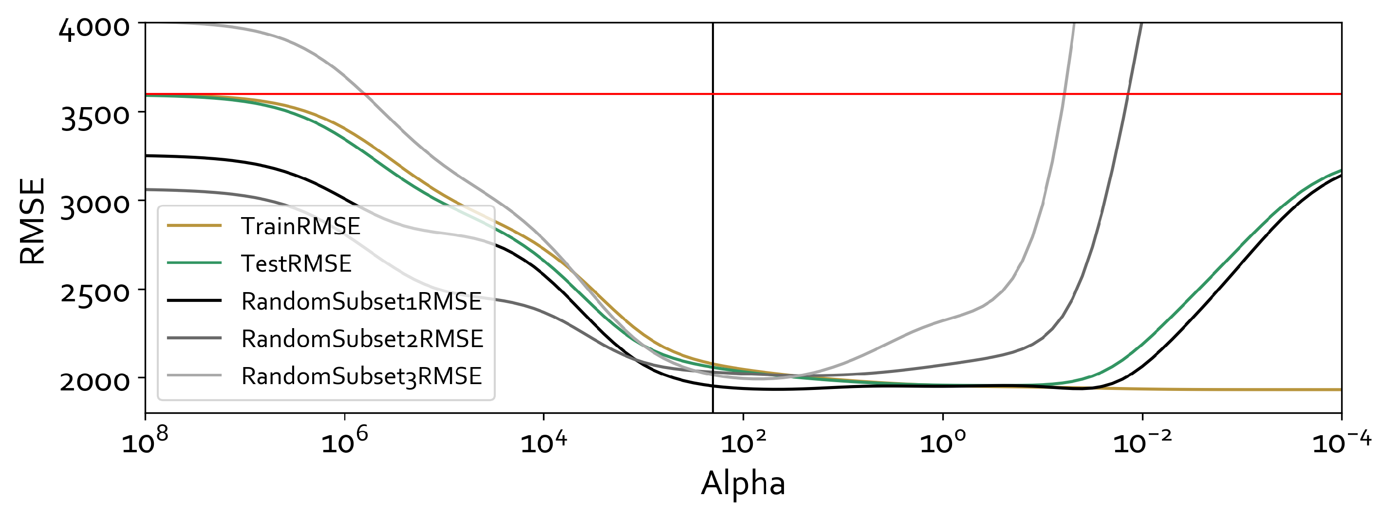
The Root Mean Squared Error (RMSE) is calculated for the training set and the test set. The RMSE is very similar for the training and cross-validation subset, which is why it is not displayed in Figure 8. The training set RMSE is the average of all three cross-validations. Additionally, three random samples of 50 observations are retrieved from the original dataset and predictions are made using the estimated coefficients at each $\mathsf{\alpha }$-level. All resulting RMSEs are displayed in Figure 8.

As mentioned above, for very large values of $\mathsf{\alpha }$, the model estimates the average of the net position. The RMSE is therefore equal to the standard deviation of the dependent variable in the training set (red horizontal line at RMSE = 3595) (Note that the standard deviation slightly deviates from the standard deviation of the net position in the overall dataset (cf. Table A1) This is because the training dataset is a subset of the overall dataset. However, the values match very closely, stemming from the stratified sampling). Here, the model suffers from underfitting and is characterized by high bias but low variance. This is confirmed by very similar RMSEs for the training and test set. For decreasing values of $\mathsf{\alpha }$, the RMSEs of all subsets diminish. For $\mathsf{\alpha }$-values too small, the model is overfitted and does not generalize well. This is reflected by a further decreasing RMSE for the training subset for very small values of $\mathsf{\alpha }$. However, the RMSE for the test subset starts to increase at an $\mathsf{\alpha }$-level of around 0.1. The RMSEs of the random subsets increase at $\mathsf{\alpha }$-levels between 100 and 0.05.

Selecting a point, for which the RMSEs of the test sets is low while avoiding an overfitted model, an $\mathsf{\alpha }$-value of 200 was chosen. At this level, the model also performs well for all random subsets. The coefficients, corresponding to $\mathsf{\alpha }=200$, were used to estimate the effect of PV and wind energy on the net position. The results are discussed in the following section.

The Ridge Regression at $\mathsf{\alpha }$-value = 200 achieves RMSEs close to the corresponding OLS regression, which means that further decreasing regularization would not substantially improve the goodness of fit. Overall, the RMSE is still high relative to the mean and standard deviation of the target variable. For accurately predicting the net position, more complex models could be deployed. For example, a regression analysis method such as LASSO (least absolute shrinkage and selection operator) is more well-suited to feature selection and model identification. However, this technique does not handle highly correlated variables well [34]. Since the goal of this analysis is measuring the marginal effects of wind and PV production on net positions, the clear interpretability of regression coefficients is preferred over higher explanatory power.

All coefficients, together with their standard deviations, t-values and p-values are displayed in

Table A3. Coefficients of the Ridge Regression at an $\mathsf{\alpha }$-level of 200. R-squared: 0.672, Adjusted R-squared: 0.671, F-statistic: 884.6.

Variable	Coefficient	Std. Error	t-Value	p-Value	Variable	Coefficient	Std. Error	t-Value	p-Value
Intercept	$5.51\times {10}^{+03}$	$3.61\times {10}^{+03}$	1.52	0.13	$Price$	$2.48\times {10}^{+01}$	$2.19\times {10}^{+01}$	1.13	0.26
$y_2$	$1.31\times {10}^{+03}$	$2.54\times {10}^{+02}$	5.14	0.00	$Wind$	$1.44\times {10}^{-01}$	$3.77\times {10}^{+02}$	3.82	0.00
$y_3$	$-6.26\times {10}^{+02}$	$7.10\times {10}^{+02}$	−0.88	0.38	$PV$	$2.04\times {10}^{-01}$	$4.10\times {10}^{+02}$	4.95	0.00
$y_4$	$2.51\times {10}^{+03}$	$1.46\times {10}^{+03}$	1.71	0.09	$Ca{p}_{\mathrm{Onshore}}$	$6.95\times {10}^{-02}$	$7.28\times {10}^{-01}$	0.09	0.92
$y_5$	$-1.01\times {10}^{+03}$	$2.56\times {10}^{+03}$	−0.39	0.69	$Ca{p}_{\mathrm{Offshore}}$	$1.14\times {10}^{-01}$	$8.78\times {10}^{+00}$	0.01	0.99
$h_2$	$2.61\times {10}^{+03}$	$3.23\times {10}^{+02}$	8.07	0.00	$Ca{p}_{\mathrm{PV}}$	$9.39\times {10}^{-02}$	$2.81\times {10}^{-01}$	0.33	0.74
$h_3$	$1.45\times {10}^{+03}$	$3.31\times {10}^{+02}$	4.38	0.00	$FB\times Load$	$-1.35\times {10}^{-02}$	$1.78\times {10}^{-02}$	−0.75	0.45
$h_4$	$-1.36\times {10}^{+03}$	$3.26\times {10}^{+02}$	−4.16	0.00	$FB\times Price$	$9.54\times {10}^{-01}$	$8.61\times {10}^{+00}$	0.11	0.91
$h_5$	$-2.41\times {10}^{+03}$	$3.27\times {10}^{+02}$	−7.36	0.00	$FB\times Wind$	$1.08\times {10}^{-01}$	$1.34\times {10}^{+02}$	8.09	0.00
$h_6$	$-9.39\times {10}^{+02}$	$3.22\times {10}^{+02}$	−2.91	0.00	$FB\times PV$	$5.99\times {10}^{-02}$	$1.09\times {10}^{+02}$	5.47	0.00
$h_7$	$-2.03\times {10}^{+03}$	$3.15\times {10}^{+02}$	−6.44	0.00	$FB\times Ca{p}_{\mathrm{Onshore}}$	$-1.35\times {10}^{-02}$	$2.24\times {10}^{-01}$	−0.06	0.95
$h_8$	$-3.99\times {10}^{+03}$	$3.24\times {10}^{+02}$	12.32	0.00	$FB\times Ca{p}_{\mathrm{Offshore}}$	$5.65\times {10}^{-01}$	$3.61\times {10}^{-01}$	1.56	0.12
$h_9$	$-2.88\times {10}^{+03}$	$3.26\times {10}^{+02}$	−8.86	0.00	$FB\times Ca{p}_{\mathrm{PV}}$	$-8.39\times {10}^{-03}$	$8.14\times {10}^{-01}$	−0.01	0.99
$h_{10}$	$-1.08\times {10}^{+03}$	$3.46\times {10}^{+02}$	−3.12	0.00	$Loa{d}^2$	$-3.20\times {10}^{-07}$	$1.70\times {10}^{-07}$	−1.96	0.05
$h_{11}$	$-1.43\times {10}^{+03}$	$3.60\times {10}^{+02}$	−3.97	0.00	$Load\times Price$	$-8.17\times {10}^{-04}$	$1.43\times {10}^{-04}$	−5.71	0.00
$h_{12}$	$-2.40\times {10}^{+03}$	$3.73\times {10}^{+02}$	−6.42	0.00	$Load\times Wind$	$-2.70\times {10}^{-07}$	$3.60\times {10}^{-07}$	−0.75	0.45
$h_{13}$	$-1.06\times {10}^{+03}$	$3.75\times {10}^{+02}$	−2.81	0.00	$Load\times PV$	$6.90\times {10}^{-07}$	$3.70\times {10}^{-07}$	1.84	0.07
$h_{14}$	$5.09\times {10}^{+02}$	$3.74\times {10}^{+02}$	1.36	0.17	$Load\times Ca{p}_{\mathrm{Onshore}}$	$-2.00\times {10}^{-08}$	$1.80\times {10}^{-06}$	0.00	0.99
$h_{15}$	$1.84\times {10}^{+03}$	$3.61\times {10}^{+02}$	5.09	0.00	$Load\times Ca{p}_{\mathrm{Offshore}}$	$-5.23\times {10}^{-06}$	$1.09\times {10}^{-05}$	−0.47	0.63
$h_{16}$	$1.52\times {10}^{+03}$	$3.57\times {10}^{+02}$	4.24	0.00	$Load\times Ca{p}_{\mathrm{PV}}$	$4.90\times {10}^{-07}$	$9.30\times {10}^{-07}$	0.52	0.60
$h_{17}$	$1.37\times {10}^{+03}$	$3.39\times {10}^{+02}$	4.03	0.00	$Pric{e}^2$	$1.09\times {10}^{-01}$	$1.41\times {10}^{-02}$	7.76	0.00
$h_{18}$	$-1.78\times {10}^{+03}$	$3.42\times {10}^{+02}$	−5.20	0.00	$Price\times Wind$	$6.54\times {10}^{-04}$	$1.48\times {10}^{-04}$	4.42	0.00
$h_{19}$	$-4.38\times {10}^{+03}$	$3.28\times {10}^{+02}$	13.35	0.00	$Price\times PV$	$2.36\times {10}^{-03}$	$1.58\times {10}^{-04}$	14.88	0.00
$h_{20}$	$-5.40\times {10}^{+03}$	$3.27\times {10}^{+02}$	16.54	0.00	$Price\times Ca{p}_{\mathrm{Onshore}}$	$1.18\times {10}^{-03}$	$1.22\times {10}^{-03}$	0.97	0.33
$h_{21}$	$-3.64\times {10}^{+03}$	$3.28\times {10}^{+02}$	11.09	0.00	$Price\times Ca{p}_{\mathrm{Offshore}}$	$-3.71\times {10}^{-03}$	$4.87\times {10}^{-03}$	−0.76	0.45
$h_{22}$	$-2.18\times {10}^{+03}$	$3.20\times {10}^{+02}$	−6.81	0.00	$Price\times Ca{p}_{\mathrm{PV}}$	$-3.14\times {10}^{-04}$	$5.69\times {10}^{-04}$	−0.55	0.58
$h_{23}$	$6.72\times {10}^{+02}$	$3.25\times {10}^{+02}$	2.06	0.04	$Win{d}^2$	$-7.10\times {10}^{-06}$	$2.80\times {10}^{-07}$	25.52	0.00
$h_{24}$	$4.04\times {10}^{+03}$	$3.22\times {10}^{+02}$	12.57	0.00	$Wind\times PV$	$1.02\times {10}^{-06}$	$3.90\times {10}^{-07}$	2.61	0.01
$m_2$	$6.04\times {10}^{+03}$	$1.83\times {10}^{+02}$	33.03	0.00	$Wind\times Ca{p}_{\mathrm{Onshore}}$	$8.50\times {10}^{-07}$	$2.24\times {10}^{-06}$	0.38	0.70
$m_3$	$2.71\times {10}^{+03}$	$1.76\times {10}^{+02}$	15.34	0.00	$Wind\times Ca{p}_{\mathrm{Offshore}}$	$-6.35\times {10}^{-05}$	$8.04\times {10}^{-06}$	−7.90	0.00
$m_4$	$-4.30\times {10}^{+03}$	$1.90\times {10}^{+02}$	22.66	0.00	$Wind\times Ca{p}_{\mathrm{PV}}$	$7.93\times {10}^{-06}$	$1.26\times {10}^{-06}$	6.29	0.00
$m_5$	$-1.29\times {10}^{+04}$	$1.95\times {10}^{+02}$	66.37	0.00	$P{V}^2$	$7.09\times {10}^{-06}$	$3.60\times {10}^{-07}$	19.79	0.00
$m_6$	$-1.03\times {10}^{+04}$	$2.13\times {10}^{+02}$	48.30	0.00	$PV\times Ca{p}_{\mathrm{Onshore}}$	$-1.10\times {10}^{-06}$	$2.18\times {10}^{-06}$	−0.50	0.61
$m_7$	$-1.21\times {10}^{+04}$	$2.26\times {10}^{+02}$	53.42	0.00	$PV\times Ca{p}_{\mathrm{Offshore}}$	$-3.29\times {10}^{-05}$	$6.36\times {10}^{-06}$	−5.16	0.00
$m_8$	$-9.16\times {10}^{+03}$	$2.44\times {10}^{+02}$	37.59	0.00	$PV\times Ca{p}_{\mathrm{PV}}$	$-2.73\times {10}^{-06}$	$1.39\times {10}^{-06}$	−1.96	0.05
$m_9$	$1.59\times {10}^{+01}$	$2.62\times {10}^{+02}$	0.06	0.95	$Ca{p}_{\mathrm{Onshore}}^2$	$5.90\times {10}^{-07}$	$1.53\times {10}^{-05}$	0.03	0.97
$m_{10}$	$2.75\times {10}^{+03}$	$2.75\times {10}^{+02}$	10.01	0.00	$Ca{p}_{\mathrm{Onshore}}\times Ca{p}_{\mathrm{Offshore}}$	$-1.45\times {10}^{-06}$	$1.46\times {10}^{-04}$	0.00	0.99
$m_{11}$	$3.69\times {10}^{+03}$	$3.07\times {10}^{+02}$	12.03	0.00	$Ca{p}_{\mathrm{Onshore}}\times Ca{p}_{\mathrm{PV}}$	$5.00\times {10}^{-07}$	$3.86\times {10}^{-05}$	0.01	0.99
$m_{12}$	$4.54\times {10}^{+03}$	$3.42\times {10}^{+02}$	13.25	0.00	$Ca{p}_{\mathrm{Offshore}}^2$	$1.25\times {10}^{-05}$	$1.40\times {10}^{-04}$	0.08	0.93
$FB$	$-1.84\times {10}^{+02}$	$6.55\times {10}^{+04}$	0.00	1.00	$Ca{p}_{\mathrm{Offshore}}\times Ca{p}_{\mathrm{PV}}$	$1.45\times {10}^{-06}$	$3.77\times {10}^{-04}$	0.00	1.00
$Load$	$-7.73\times {10}^{-03}$	$2.85\times {10}^{-02}$	−0.27	0.79	$Ca{p}_{\mathrm{PV}}$	$-9.80\times {10}^{-07}$	$5.72\times {10}^{-06}$	−0.17	0.86

. Note that especially the variables with very high VIFs (cf. Table A2) are characterized by small coefficients relative to their standard deviations and are consequently insignificant.

6. Results and Discussion

The effect of PV and wind generation on the net position is estimated for different levels of PV and wind generation. For this, the 10th percentile, the mean and 90th percentile of the distribution of PV and wind generation are inserted into the partial derivatives described in Equations (2) and (3). Additionally, the effects are calculated with and without the effect of the flow-based dummy variable. Note that for all other explanatory variables, the average value of the training dataset is inserted, i.e., 63.8 GW for load, 34.87 EUR for price and 35.6 GW, 34.8 GW and 1.49 GW for PV, wind onshore and wind offshore capacities, respectively. Slight deviations from average values in Table A1 are due to using a subset as training data. For PV the low (73 MW), average (6721 MW) and high (16,755 MW) values are taken from a subset of the training data which only contains situations with PV generation greater than 0. In the overall dataset, the mean and 10th percentile are equal to 0. For wind, low (1240 MW), average (7205 MW) and high (16,341 MW) values are extracted from the full training set.

The effects of one additional unit of PV and wind generation, respectively, for the different levels of PV and wind generation are displayed in

Table 2. Results from the Ridge Regression at $\mathsf{\alpha }=200$: displayed are the effects of one additional unit of PV and wind generation, respectively, for different levels of PV and wind generation. Values including the effect of flow-based market coupling are in parentheses. Source: own diagram.

	Effect of PV Generation			Effect of Wind Generation
	Low PV	Average PV	High PV	Low PV	Average PV	High PV
Low	0.1473	0.2415	0.3837	0.3497	0.3565	0.3668
wind	(0.2072)	(0.3014)	(0.4436)	(0.4580)	(0.4648)	(0.4751)
Average	0.1534	0.2476	0.3898	0.2650	0.2718	0.2821
wind	(0.2133)	(0.3075)	(0.4497)	(0.3733)	(0.3801)	(0.3904)
High	0.1628	0.2570	0.3991	0.1353	0.1421	0.1524
wind	(0.2227)	(0.3169)	(0.4590)	(0.2436)	(0.2504)	(0.2607)

. The values in parentheses represent the values for situations after the introduction of flow-based market coupling. All values can be interpreted as the average fraction of an additional unit of PV or wind energy that is exported, holding everything else constant.

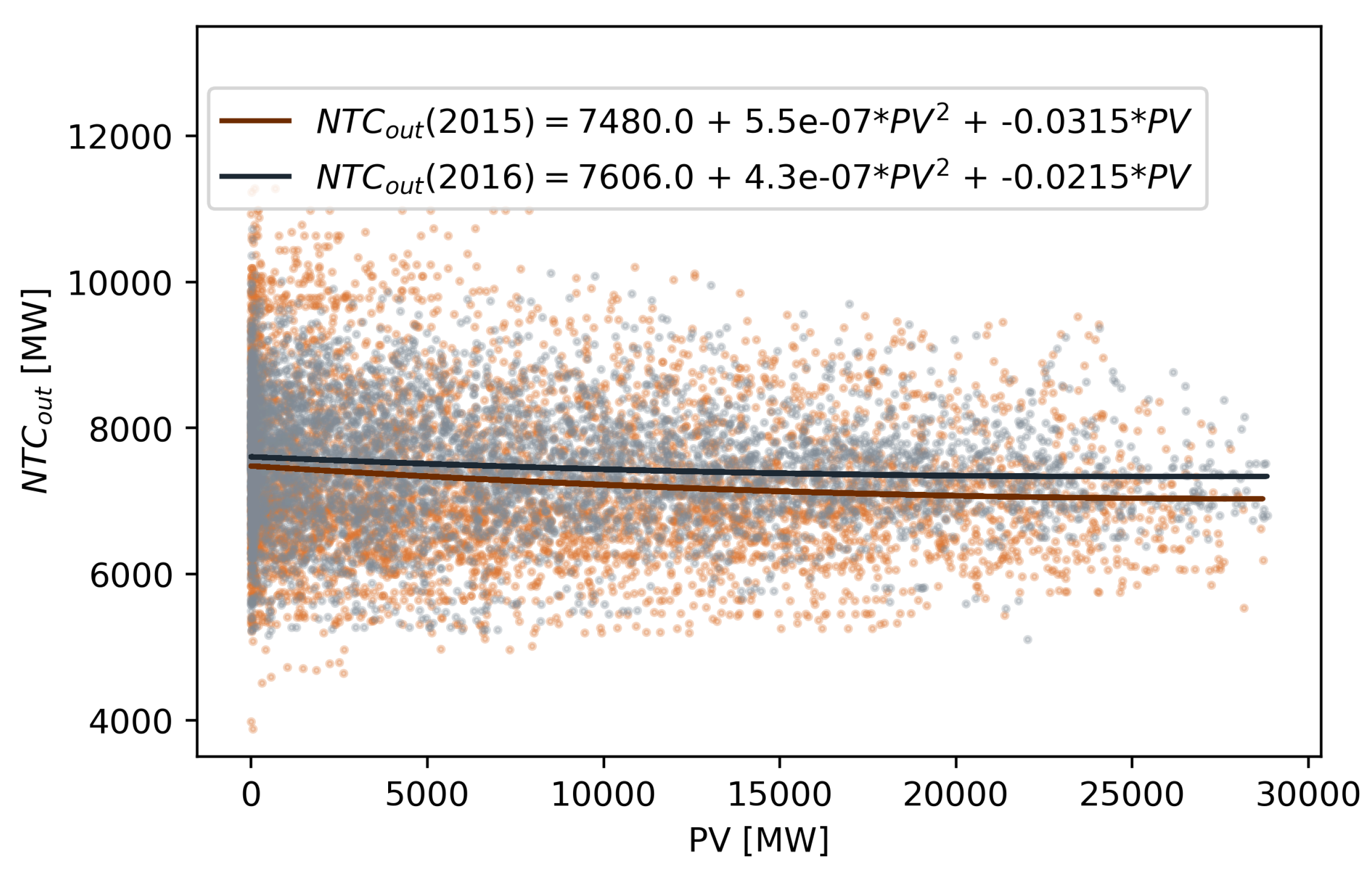
The fraction of PV generation that is exported correlates positively with overall PV generation as well as overall wind generation. However, the difference in the effect is much more pronounced for higher levels of PV production, while higher wind production only has a slight effect on the amount of PV energy being exported. This implies that the level of wind generation does not have a large impact on the fraction of PV exported while the level of PV generation significantly impacts the fraction of PV exported. The fraction of wind generation that is exported correlates positively with overall PV generation, although the effect is insubstantial. Interestingly, the amount of wind energy that is exported correlates negatively with overall wind generation. A possible explanation for this interesting result could involve the impact of wind generation on the available cross-border transfer capacities. At times when large amounts of wind feed-in is expected, it is anticipated that the grid operators will restrict the available trade capacities to limit the magnitude of loop flows. Consequently, this would reduce the fraction of wind that can be exported. The impact is expected to be more pronounced at times of high wind generation. NTC (Net Transfer Capacity) refers to the available interconnector capacities for cross-border commercial exchange.

To investigate this possible explanation further, a bi-variate regression of the variable $NT{C}_{out}$ (available NTC capacity for export) on wind and PV, respectively, is carried out. To analyze the relationship, a quadratic model is employed. Figure 9 displays the results of the regression of $NT{C}_{out}$ on wind generation. The regression indicates an inverse relationship between wind generation and the available transfer capacity, i.e., at times of high wind generation, grid constraints reduce the level of transfer capacity available for cross-border trade. The quadratic term of the regression has a negative coefficient for wind while a positive (and significantly smaller value) for PV (Figure 10). This implies that the rate of reduction of $NT{C}_{out}$ is higher at higher levels of wind generation. This finding seems to support the explanation posited above that at times of high wind generation the export of an extra unit of wind is restricted due to constraints on the available transfer capacity.

Returning to results of the Ridge Regression, the sensitivity of the results to changes in load and price are tested. The ${\mathsf{\xi }}_{10}$-coefficient, which corresponds to the interaction term $Loa{d}_t\times Win{d}_t$ is equal to $-2.7\times {10}^{-7}$. Consequently, even an increase of 10 GW in load would merely subtract $-0.0027$ from the exported wind shares. Similarly, an additional load of 10 GW would add $0.0069$ to the exported PV shares (${\mathsf{\xi }}_{11}=6.9\times {10}^{-7}$). An increase in the day-ahead price of 10 EUR raises the fraction of exported wind energy by 0.0065 (${\mathsf{\xi }}_{16}=6.54\times {10}^{-4}$) and the fraction of PV energy by 0.0236 (${\mathsf{\xi }}_{17}=2.36\times {10}^{-3}$). Thus, the results do not appear to change substantially in high or low load situations. Merely the volumes of PV shares exported increase substantially with higher prices, while the amount of exported wind production remains nearly constant in varying price regimes.

Finally, addressing the question as to the effect of the introduction of FBMC in mid-2015, the results from the regression model indicate somewhat unexpectedly a higher impact of FBMC with respect to the effect of an extra unit of wind generation (ca. 0.11) compared to PV generation (ca. 0.06). This is consistent across all regimes of wind and PV generation. In terms of an explanation, it seems plausible that owing to the fact that PV generation is more prevalent in situations with a more highly constrained network (during the day), the domain of FBMC is more strongly confined. This largely negates the impact of FBMC on cross-border flows. However, as wind generation varies across day and night, occurring in both constrained and unconstrained situations, FBMC increases the available cross-border capacity more significantly, thereby influencing cross-border commercial flows to a greater extent.

7. Conclusions and Outlook for Further Research

The preceding analysis has brought together two strains of literature currently attracting much attention in academic as well as policy circles. The effects of growing shares of VRE in power systems on prices and in turn commercial exchanges between neighboring countries, as well as the ongoing push towards integrating national markets across Europe to achieve gains in welfare. As an example of this confluence, the paper pursues the questions as to the effects of wind and solar energy generation on the commercial export surplus in Germany that has seen exponential growth in recent years. Possible impacts related to the introduction of Flow Based Market Coupling as a means of exploiting physical interconnectors between Germany and its neighbours are also investigated.

The results of the empirical regression model offer the following conclusions. As pertains to PV, the share of generation that is exported is positively correlated with overall PV, as well as wind generation levels, whereby the effect is much more pronounced for high levels of PV production. In the case of wind generation, the share of wind generation being exported also is positively correlated with overall wind generation. However, the effect is minimal. In contrast to PV, the additional unit of wind energy being exported is negatively correlated with overall wind production. Changing the underlying load situations in the data does not significantly affect these results. A possible explanation posited for this result involves the relationship between wind and PV generation and available transfer capacities. While PV generation is observed to have a very limited impact on the available cross-border export capacity, wind generation sharply reduces it. Furthermore, it is observed that at times of higher wind generation this effect is more pronounced. Furthermore, the analysis imparts the insight that the effect of the introduction of FBMC in the CWE region in mid-2015 has had a statistically significant yet minimal impact on German electricity exports. However, the effect of FBMC in conjunction with PV and wind production is more pronounced, with its greatest effect found to be in combination with wind generation.

The preceding analysis offers several avenues for further research. The differences in the impact of PV and wind generation on cross-border trade has been largely neglected in the extant literature. Understanding these dynamics is important for policy makers when designing incentives that facilitate an efficient integration of VRE sources. As grid and market integration are advanced further, these aspects are set to gain in importance with increasing cross-border interactions. Furthermore, implications regarding quantifying resulting welfare effects present an additional aspect worth considering in future work on the topic. With the pending phase-out of the coal power fleet in Germany, the effect of this policy action on cross-border trade developments in the future would also be an interesting supplemental analysis to the one undertaken here. The analysis undertaken primarily looks at prices, VRE capacity and generation within Germany. Future research should consider adaptations in the electricity system in neighboring countries, while providing a more detailed representation of interconnector availabilities.