Large Eddy Simulations of the Flow Fields over Simplified Hills with Different Roughness Conditions, Slopes, and Hill Shapes: A Systematical Study


Abstract
1. Introduction
2. Numerical Model
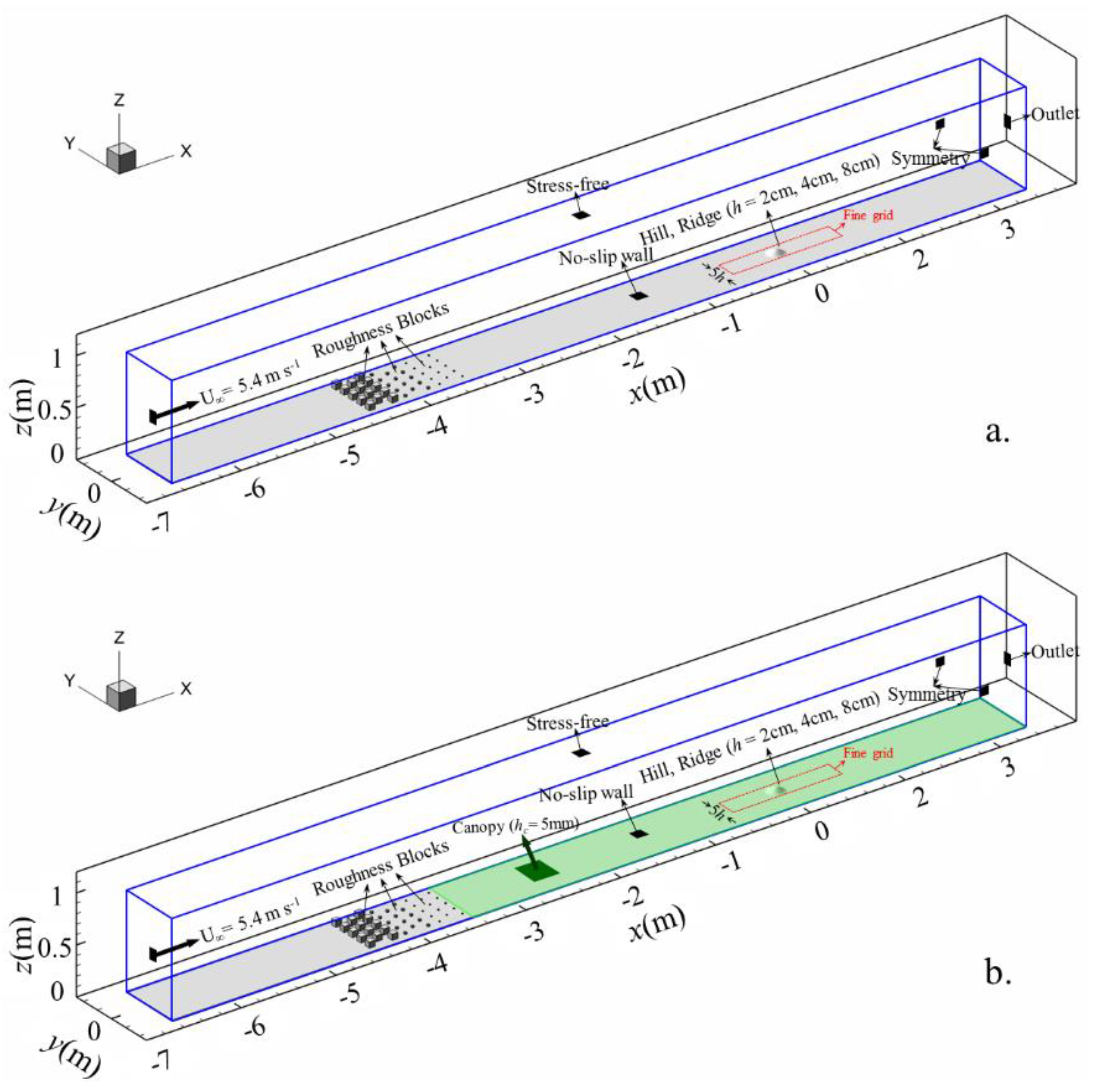
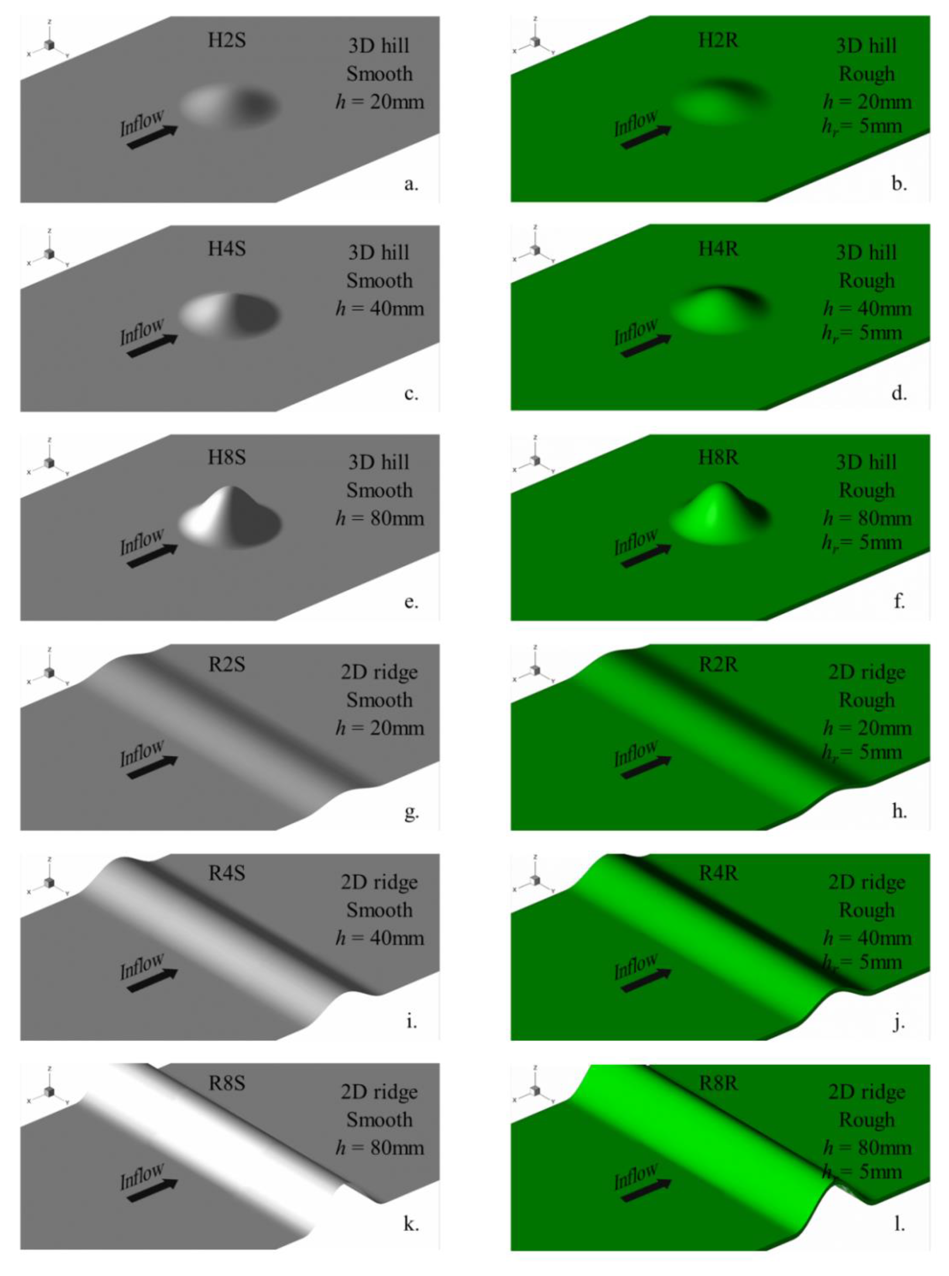
2.1. Configurations
2.2. Numerical Method
2.2.1. Governing Equations
2.2.2. Method Modeling Roughness
2.2.3. Boundary Conditions
2.2.4. Grid System
2.2.5. Solution Schemes
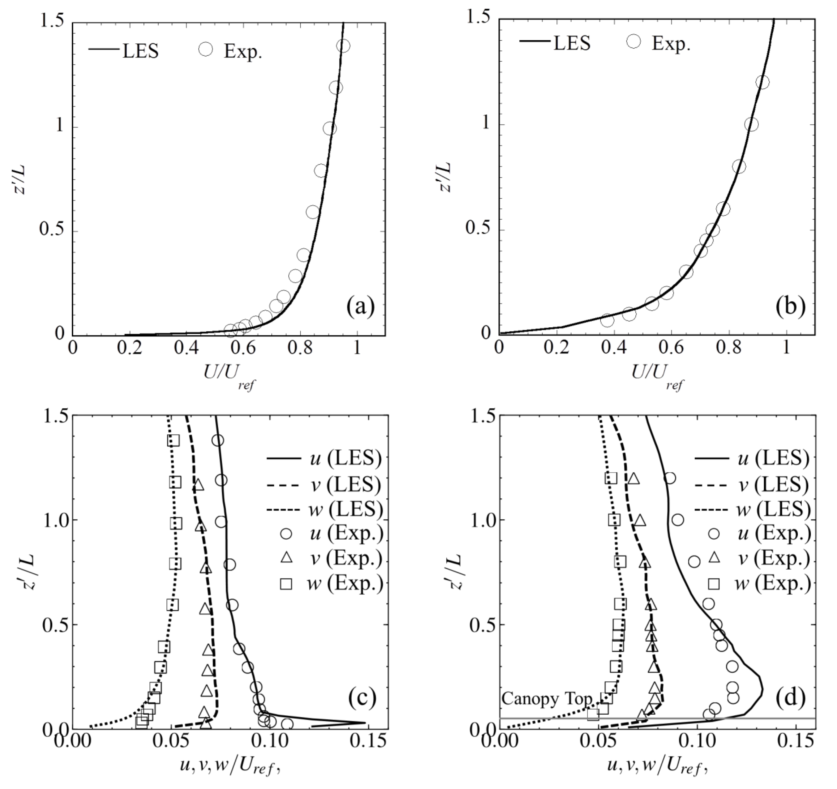
2.3. Upcoming TBL
3. Numerical Results
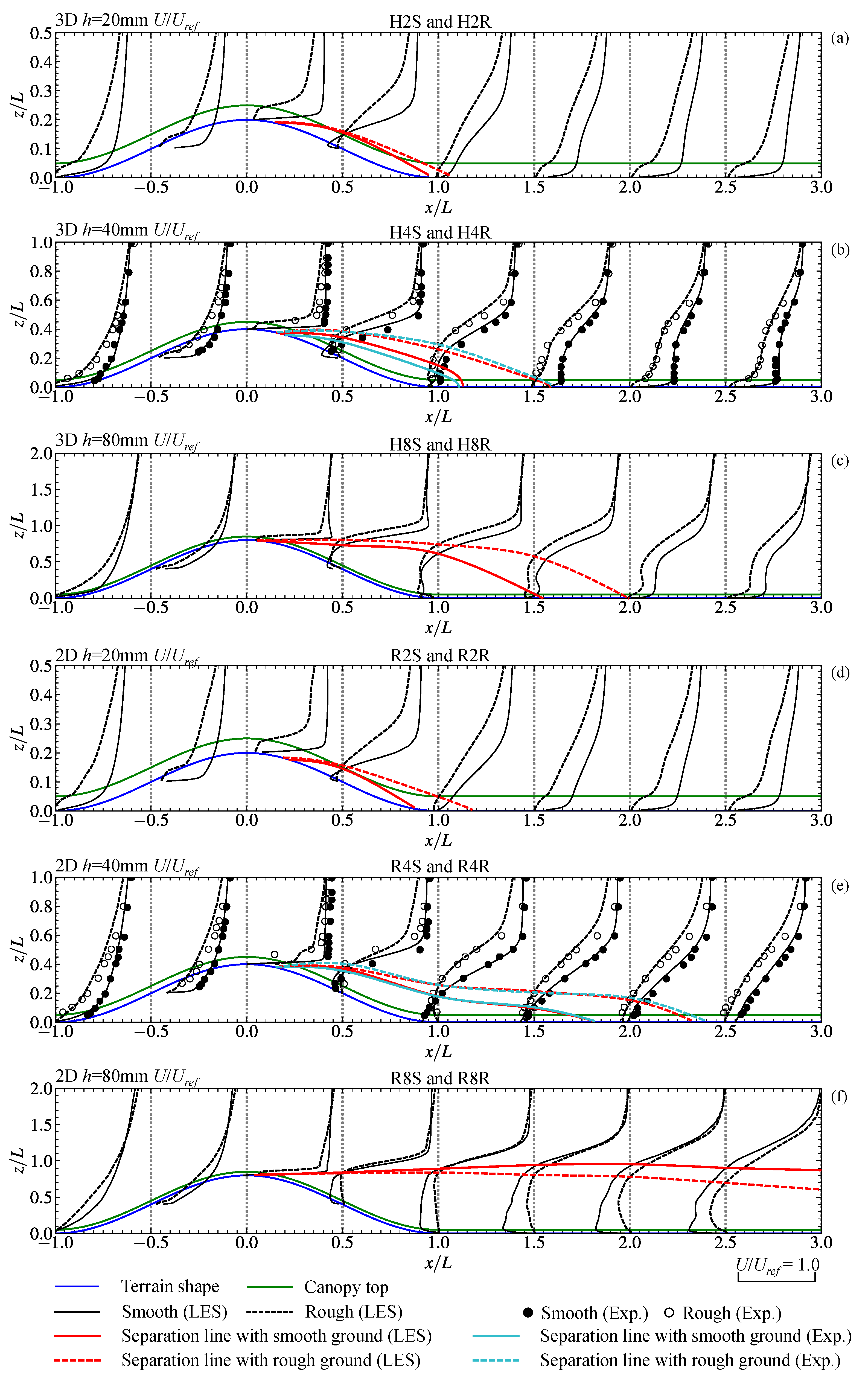
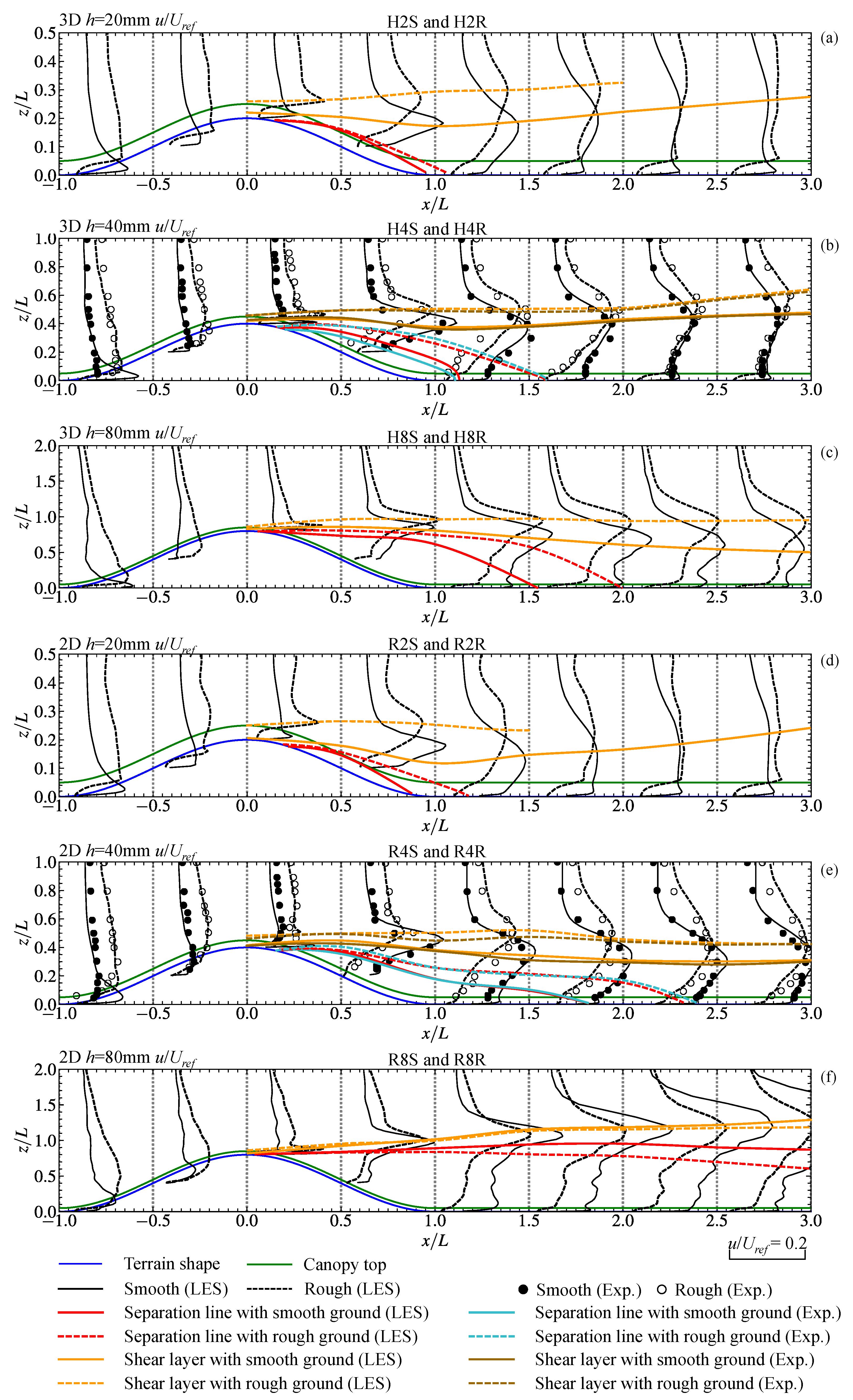
3.1. Mean Streamwise Velocity
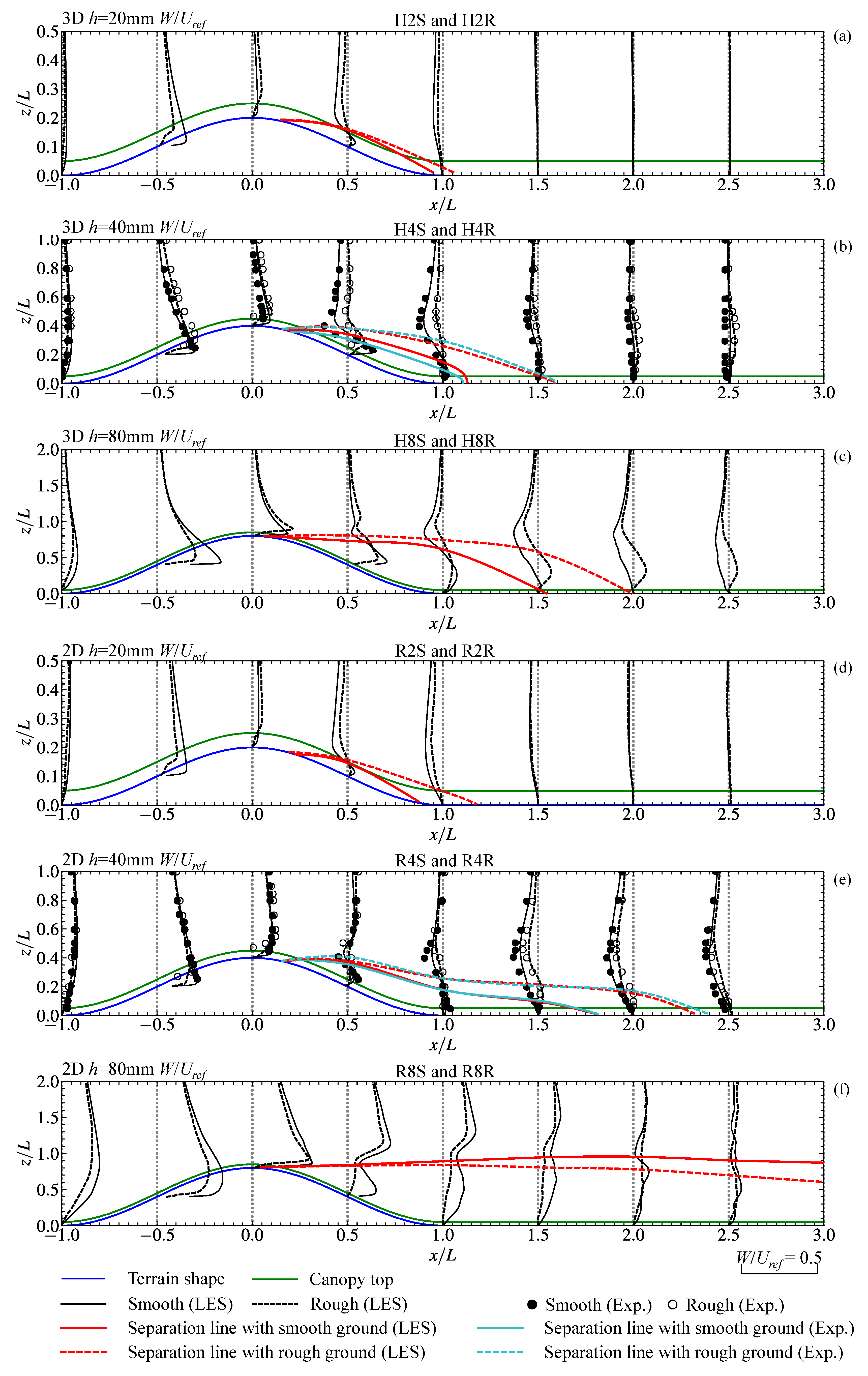
3.2. Mean Vertical Velocity
3.3. Fluctuations of Streamwise Velocity
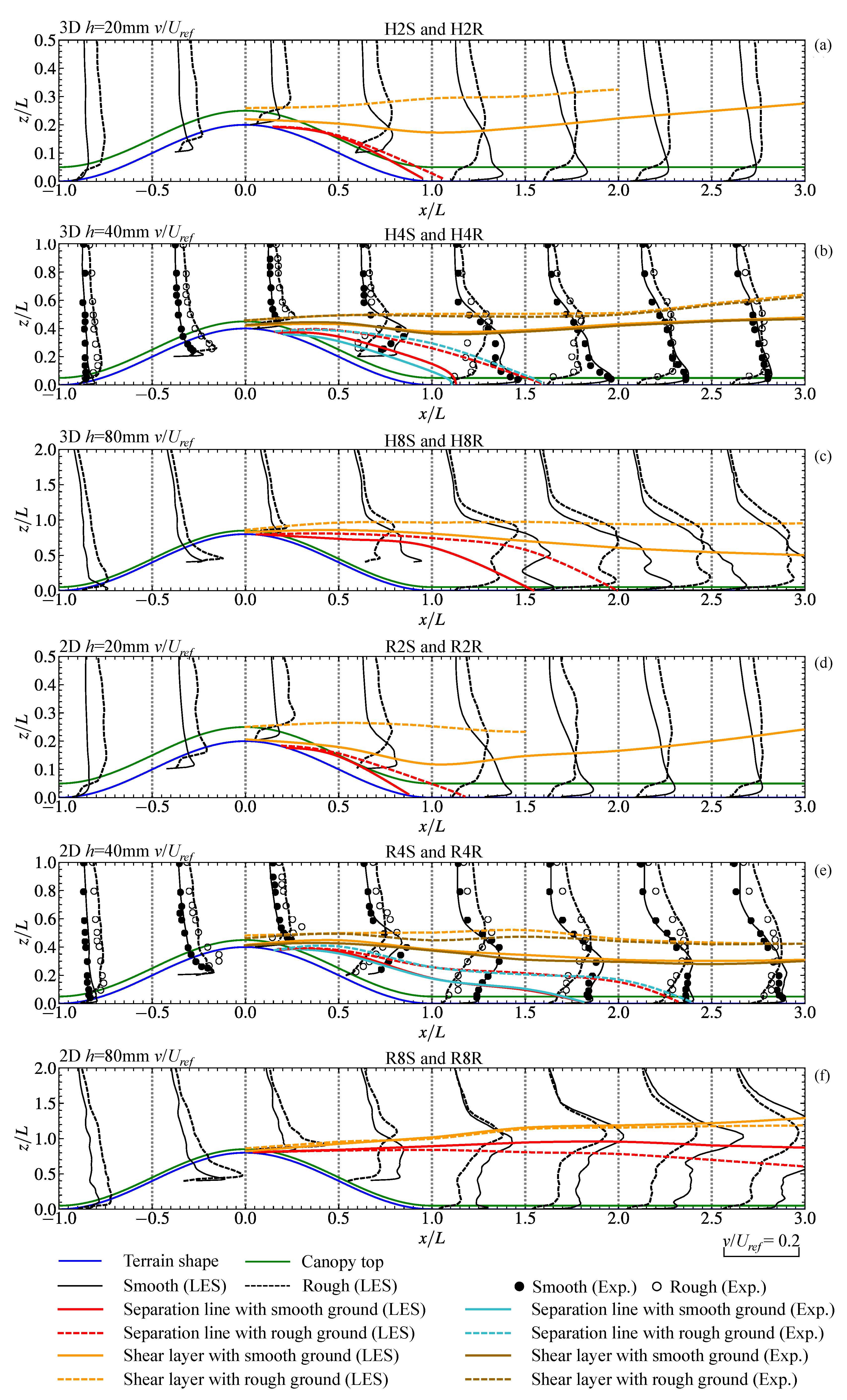
3.4. Fluctuations of Spanwise Velocity
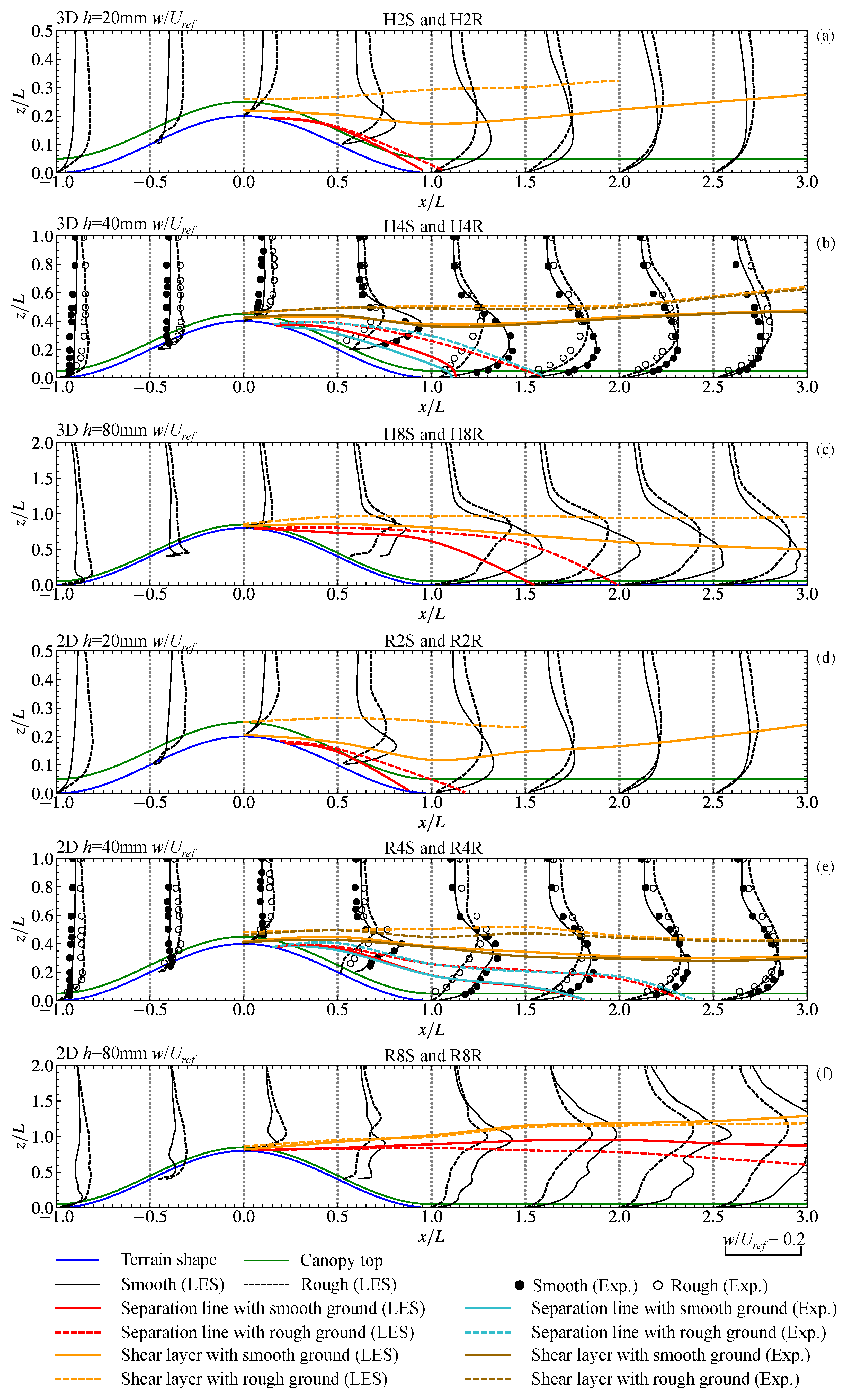
3.5. Fluctuations of Vertical Velocity
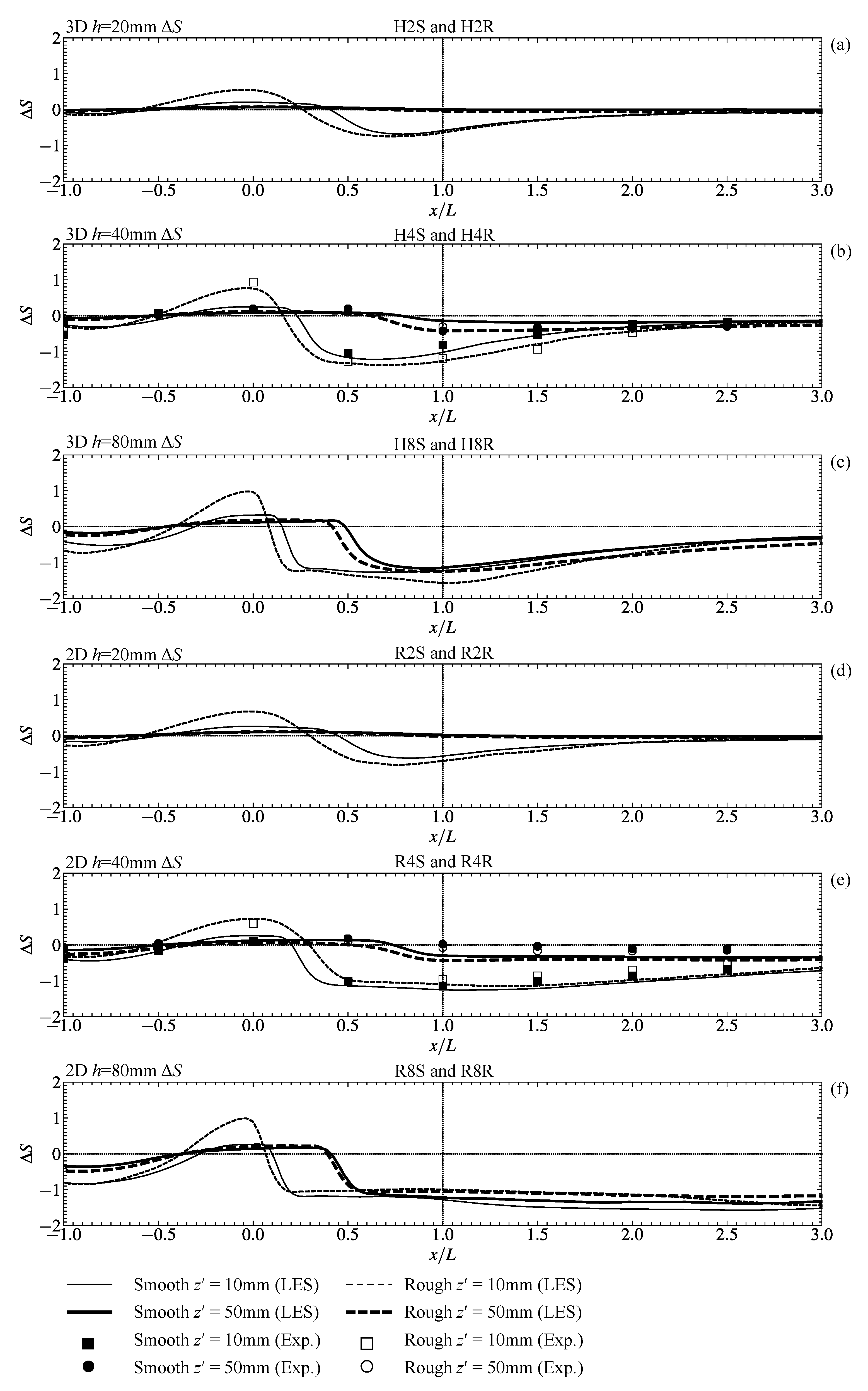
3.6. Fractional Speed-Up Ratio
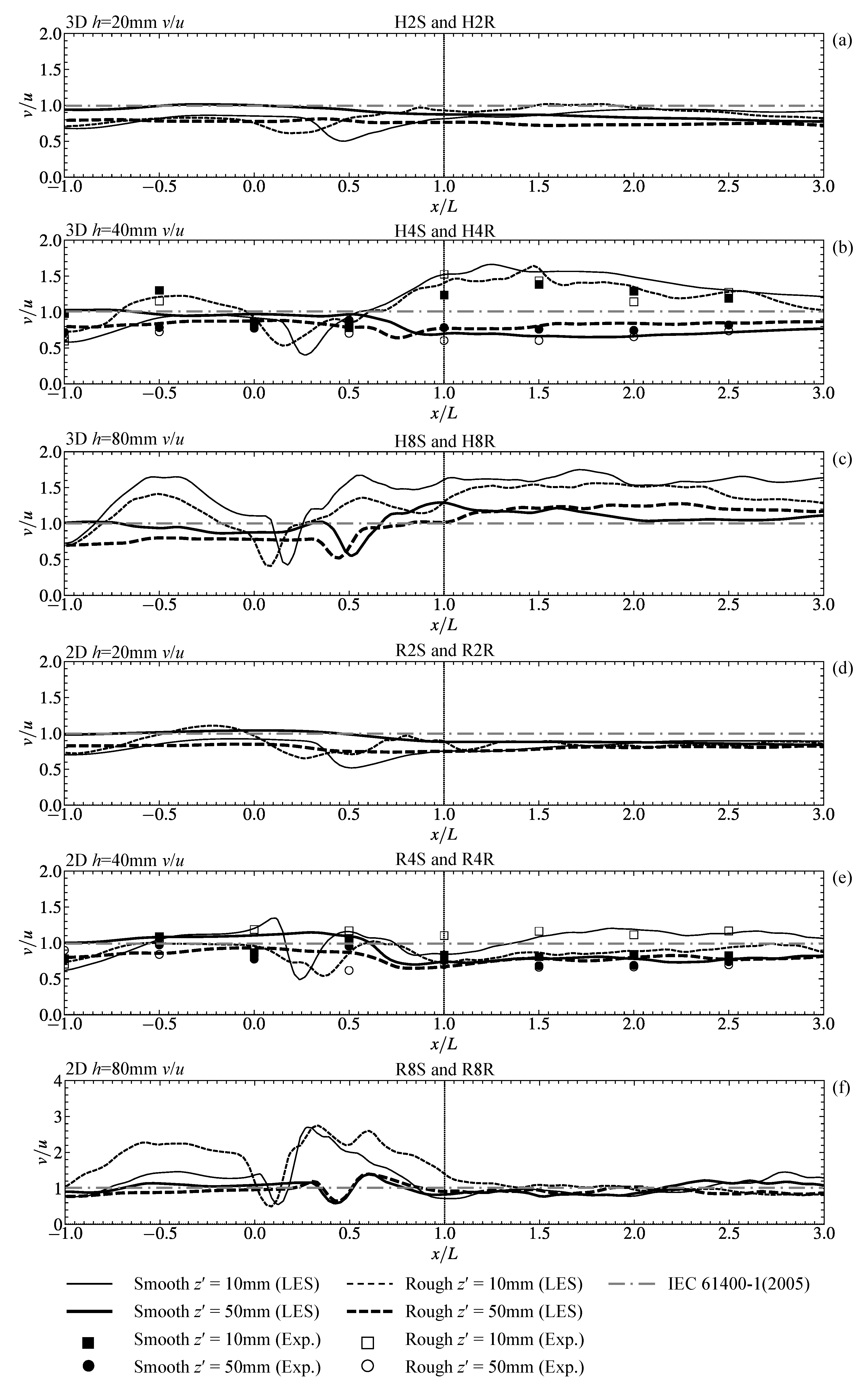
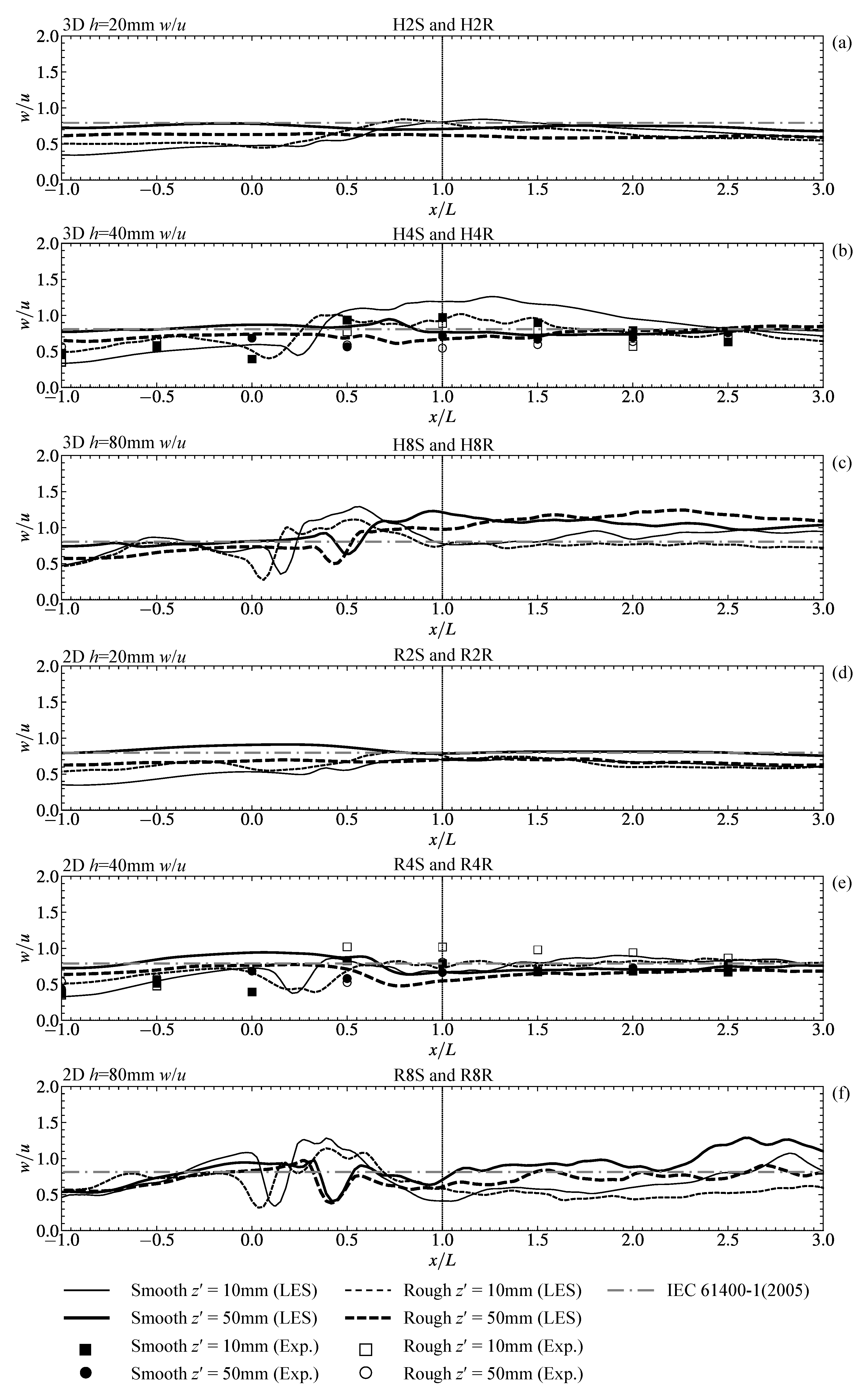
3.7. Fluctuation Ratios
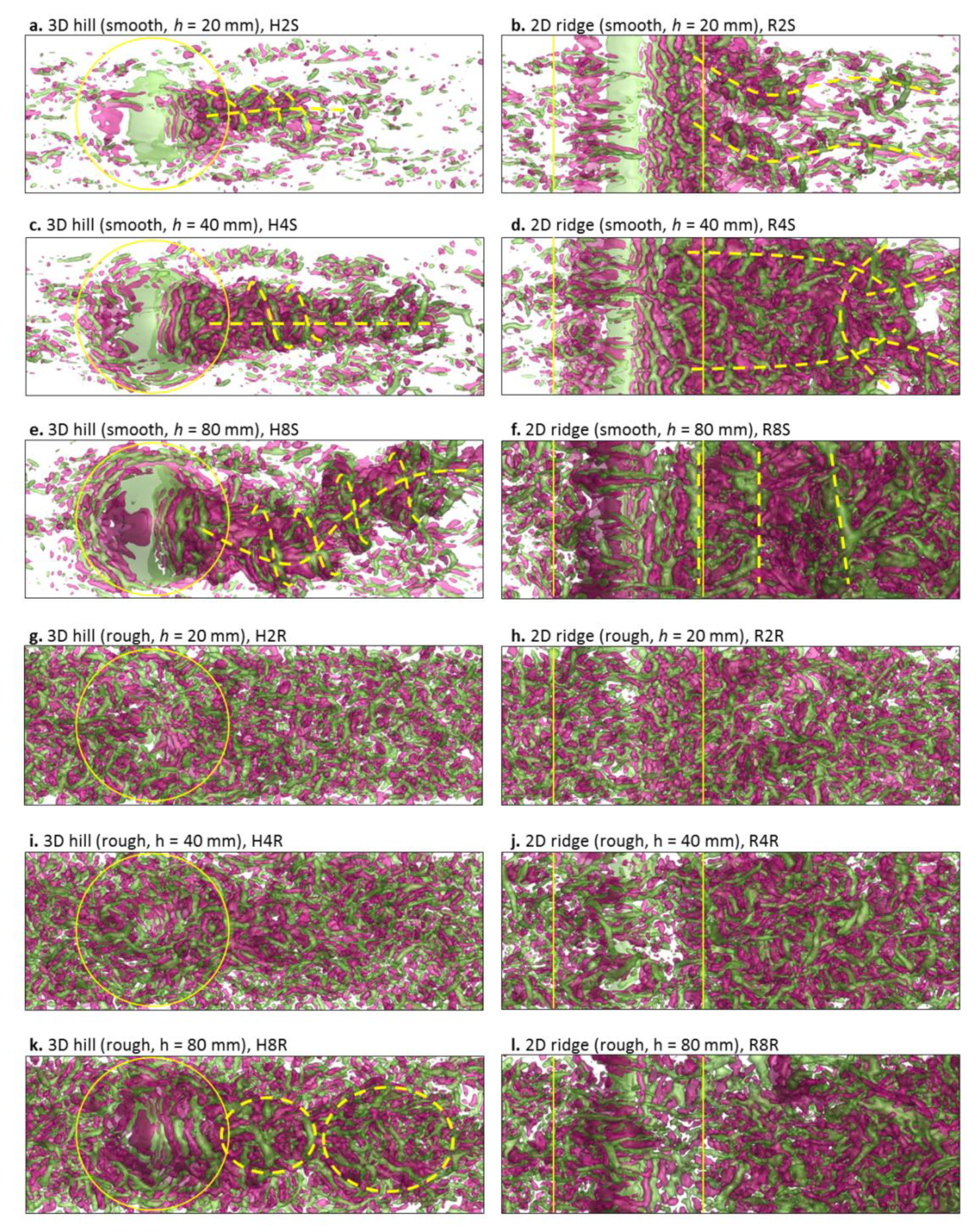
3.8. Instantaneous Flow Fields
4. Conclusions
- 1)
- For the mean streamwise velocity, as the hill slope increases, the roughness effects get weaker; however, the hill shape effects become more evident. And if the hill is very steeply-sloped, the roughness effects will be further weakened as the hill changes from 3D to 2D.
- 2)
- For the mean vertical velocity, the distortion of the profiles owing to the ground roughness is strengthened for the steeper hills, while it seems to be weakened as the hill alters from 3D to 2D. Importantly, at the hill summits, the acceleration of W as increasing the slope becomes quicker for 2D hills.
- 3)
- For the fluctuations, at the summit, u seems to be restrained as increasing the slope, which is more obvious when the hill shape is 3D or the ground is rough. After changing the hill shape to 2D, the location of the peak u is lower than the corresponding 3D hills. Two peaks on v profiles still appear but become less obvious when the ground is rough. In addition, as increasing the hill slope, these two peaks turn more obvious.
- 4)
- For the fractional speed-up ratio, at the summit of rough hills can reach to three times as large as that over the corresponding smooth hills. With increasing the hill slope, at the summit increases obviously. However, the hill shape shows unapparent effects on the maximum at the summit. In addition, the area with positive becomes smaller as the hill gets steeper.
- 5)
- For the fluctuation ratios, the introduction of ground roughness can hardly affect v/u, and the underestimation of v/u by IEC 61400-1 in the hill wake is quite obvious when the hill shape is 3D [35]. After changing the hill shape from 3D to 2D, v/u becomes almost equal as those in the guideline.
- 6)
- For the turbulence structures, clear coherent turbulence structure can be identified for smooth 3D hills, and as increasing the hills slope, the major core of the coherent structure tends to show large spanwise sway motions. For 2D hills, when the ground is smooth and the slope is low, the major core of the wake vortex is nearly perpendicular to the ridge line, and as increasing the hill slope, a kind of ejection-sweep structure of large scale occurs. Further increasing the hill slope, a wavy structure with the major core being parallel with the ridge line appears. After introducing the ground roughness, the clear coherent turbulence structures are broken into small eddies.
Author Contributions
Funding
Acknowledgments
Conflicts of Interest
References
- Politis, E.; Prospathopoulos, J.; Cabezon, D.; Hansen, K.; Chaviaropoulos, P.; Barthelmie, R. Modeling wake effects in large wind farms in complex terrain: The problem, the methods and the issues. Wind Energy 2011, 15, 161–182. [Google Scholar] [CrossRef]
- Carvalho, A.; Carvalho, A.; Gelpi, I.; Barreiro, M.; Borrego, C.; Miranda, A.; Pérez-Muñuzuri, V. Influence of topography and land use on pollutants dispersion in the Atlantic coast of Iberian Peninsula. Atmos. Environ. 2006, 40, 3969–3982. [Google Scholar] [CrossRef]
- Davenport, A.G.; King, J.P.C. The influence of topography on the dynamic wind loading of long span bridges. J. Wind Eng. Ind. Aerodyn. 1990, 36, 1373–1382. [Google Scholar] [CrossRef]
- Matusick, G.; Ruthrof, K.; Brouwers, N.; Hardy, G. Topography influences the distribution of autumn frost damage on trees in a Mediterranean-type Eucalyptus forest. Trees 2014, 28, 1449–1462. [Google Scholar] [CrossRef]
- Loureiro, J.; Alho, A.; Freire, A. The numerical computation of near-wall turbulent flow over a steep hill. J. Wind Eng. Ind. Aerodyn. 2008, 96, 540–561. [Google Scholar] [CrossRef]
- Britter, R.; Hunt, J.B.; Richards, K. Air flow over a two-dimensional hill: Studies of velocity speed-up, roughness effects and turbulence. Q. J. R. Meteorol. Soc. 1981, 107, 91–110. [Google Scholar] [CrossRef]
- Pearse, J.; Lindley, D.; Stevenson, D. Wind flow over ridges in simulated atmospheric boundary layers. Bound.-Layer Meteorol. 1981, 21, 77–92. [Google Scholar] [CrossRef]
- Brown, A.; Hobson, J.; Wood, N. Large-eddy simulation of neutral turbulent flow over rough sinusoidal ridges. Bound.-Layer Meteorol. 2001, 98, 411–441. [Google Scholar] [CrossRef]
- Athanassiadou, M.; Castro, I. Neutral flow over a series of rough hills: A laboratory experiment. Bound.-Layer Meteorol. 2001, 101, 1–30. [Google Scholar] [CrossRef]
- Finnigan, J.; Belcher, S. Flow over a hill covered with a plant canopy. Q. J. R. Meteorol. Soc. 2004, 130, 1–29. [Google Scholar] [CrossRef]
- Ross, A.; Vosper, S. Neutral turbulent flow over forested hills. Q. J. R. Meteorol. Soc. 2005, 131, 1841–1862. [Google Scholar] [CrossRef]
- Cao, S.; Tamura, T. Experimental study on roughness effects on turbulent boundary layer flow over a two-dimensional steep hill. J. Wind Eng. Ind. Aerodyn. 2006, 94, 1–19. [Google Scholar] [CrossRef]
- Cao, S.; Tamura, T. Effects of roughness blocks on atmospheric boundary layer flow over a two-dimensional low hill with/without sudden roughness change. J. Wind Eng. Ind. Aerodyn. 2007, 95, 679–695. [Google Scholar] [CrossRef]
- Ross, A. Large-eddy simulations of flow over forested ridges. Bound.-Layer Meteorol. 2008, 128, 59–76. [Google Scholar] [CrossRef]
- Okaze, T.; Ono, A.; Mochida, A.; Kannuki, Y.; Watanabe, S. Evaluation of turbulent length scale within urban canopy layer based on LES data. J. Wind Eng. Ind. Aerodyn. 2015, 144, 79–83. [Google Scholar] [CrossRef]
- Loureiro, J.; Freire, A. Note on a parametric relation for separating flow over a rough hill. Bound.-Layer Meteorol. 2009, 131, 309–318. [Google Scholar] [CrossRef]
- Takahashi, T.; Ohtsu, T.; Yassin, M.; Kato, S.; Murakami, S. Turbulence characteristics of wind over a hill with a rough surface. J. Wind Eng. Ind. Aerodyn. 2002, 90, 1697–1706. [Google Scholar] [CrossRef]
- Tamura, T.; Okuno, A.; Sugio, Y. Les analysis of turbulent boundary layer over 3d steep hill covered with vegetation. J. Wind Eng. Ind. Aerodyn. 2007, 95, 1463–1475. [Google Scholar] [CrossRef]
- Cao, S.; Wang, T.; Ge, Y.; Tamura, Y. Numerical study on turbulent boundary layers over two-dimensional hills-effects of surface roughness and slope. J. Wind Eng. Ind. Aerodyn. 2012, 104, 342–349. [Google Scholar] [CrossRef]
- Liu, Z.; Ishihara, T.; He, X.; Niu, H. LES study on the turbulent flow fields over complex terrain covered by vegetation canopy. J. Wind Eng. Ind. Aerodyn. 2016, 155, 60–73. [Google Scholar] [CrossRef]
- Finardi, S.; Brusasca, G.; Morselli, M.; Trombetti, F.; Tampieri, F. Boundary-layer flow over analytical two-dimensional hills: A systematic comparison of different models with wind tunnel data. Bound.-Layer Meteorol. 1993, 63, 259–291. [Google Scholar] [CrossRef]
- Hu, P.; Li, Y.; Han, Y.; Cai, S.; Xu, X. Numerical simulations of the mean wind speeds and turbulence intensities over simplified gorges using the SST k-ω turbulence model. Eng. Appl. Comput. Fluid Mech. 2016, 10, 361–374. [Google Scholar] [CrossRef]
- Ma, Y.; Liu, H. Large-eddy simulations of atmospheric flows over complex terrain using the immersed-boundary method in the weather research and forecasting model. Bound.-Layer Meteorol. 2017, 165, 421–445. [Google Scholar] [CrossRef]
- Ferreira, A.; Lopes, A.; Viegas, D.; Sousa, A. Experimental and numerical simulation of flow around two-dimensional hills. J. Wind Eng. Ind. Aerodyn. 1995, 54, 173–181. [Google Scholar] [CrossRef]
- Griffiths, A.; Middleton, J. Simulations of separated flow over two-dimensional hills. J. Wind Eng. Ind. Aerodyn. 2010, 98, 155–160. [Google Scholar] [CrossRef]
- Neff, D.; Meroney, R. Wind-tunnel modeling of hill and vegetation influence on wind power availability. J. Wind Eng. Ind. Aerodyn. 1998, 74, 335–343. [Google Scholar] [CrossRef]
- Pirooz, A.; Flay, R. Comparison of speed-up over hills derived from wind-tunnel experiments, wind-loading standards, and numerical modelling. Bound.-Layer Meteorol. 2018, 168, 213–246. [Google Scholar] [CrossRef]
- Ishihara, T.; Fujino, Y.; Hibi, K. A wind tunnel study of separated flow over a two-dimensional ridge and a circular hill. J. Wind Eng. 2001, 89, 573–576. [Google Scholar]
- Lubitz, W.; White, B. Wind-tunnel and field investigation of the effect of local wind direction on speed-up over hills. J. Wind Eng. Ind. Aerodyn. 2007, 95, 639–661. [Google Scholar] [CrossRef]
- Liu, Z.; Ishihara, T.; Tanaka, T.; He, X. LES study of turbulent flow fields over a smooth 3-D hill and a smooth 2-D ridge. J. Wind Eng. Ind. Aerodyn. 2016, 153, 1–12. [Google Scholar] [CrossRef]
- Ishihara, T.; Qi, Y. Numerical study of turbulent flow fields over steep terrains by using a modified delayed detached eddy simulations. Bound.-Layer Meteorol. 2019, 170, 45–68. [Google Scholar] [CrossRef]
- Ishihara, T.; Kazuki, H.; Susumu, O. A wind tunnel study of turbulent flow over a three-dimension steep hill. J. Wind Eng. Ind. Aerodyn. 1999, 83, 95–107. [Google Scholar] [CrossRef]
- Ferziger, J.H.; Peric, M. Computational Methods for Fluid Dynamics. Phys. Today 1997, 50, 80–84. [Google Scholar] [CrossRef]
- Liu, Z.; Cao, S.; Liu, H.; Ishihara, T. Large-Eddy simulations of the flow over an isolated three-dimensional hill. Bound.-Layer Meteorol. 2019, 170, 415–441. [Google Scholar] [CrossRef]
- IEC, Wind turbines—Part 1: design requirements 61400−1, 3rd ed.; International Electrotechnical Commission: Geneva, Switzerland, 2005.


| Case Name. | Shape | Ground Condition | Height of Hill h (mm) | Validation Case |
|---|---|---|---|---|
| H2S | 3D hill | smooth | 20 | |
| H4S | 3D hill | smooth | 40 | √ |
| H8S | 3D hill | smooth | 80 | |
| H2R | 3D hill | rough | 20 | |
| H4R | 3D hill | rough | 40 | √ |
| H8R | 3D hill | rough | 80 | |
| R2S | 2D ridge | smooth | 20 | |
| R4S | 2D ridge | smooth | 40 | √ |
| R8S | 2D ridge | smooth | 80 | |
| R2R | 2D ridge | rough | 20 | |
| R4R | 2D ridge | rough | 40 | √ |
| R8R | 2D ridge | rough | 80 |
| Locations | Boundary Type | Expression |
|---|---|---|
| Outlet of the domain | Outflow | , |
| Lateral sides of the domain | Symmetry | , , , |
| Top of the domain | Symmetry | , , , |
| Inlet of the domain | Velocity inlet | = 5.4 m·s−1,, , |
| Ground | Non-slip wall | , |
| Ground Condition | Horizontal Grid Resolution in Fine Grid Domain | Horizontal Grid Resolution in Coarse Grid Domain | Size of Fine Grid Domain | Grid Number | ||
|---|---|---|---|---|---|---|
| (mm) | (mm) | (mm) | (mm) | L | ||
| Smooth | 0.1 | 0.1 | 2 | 10 | (12, 2, 3) | 2.2 |
| Rough | 0.5 | 0.5 | 2 | 10 | (12, 2, 3) | 2.45 |
| Time-discretization scheme | Second-order implicit scheme | Cs number | 0.1 |
| Space-discretization scheme | Finite-volume method Second-order central-difference scheme | SGS model | Smagorinsky-Lilly |
| Non-dimensional time step size: Δt* = Δt/L | 0.0058 | CFL number: ΔtΣui/Δxi | <2 |
| Turbulence model | LES | Software | ANSYS Fluent 14.0 |
| Time for statistics | 400Δt* | Solution of the linearized equations | Preconditioned Conjugate Gradient + Algebraic Multigrid |
| Ground Condition | Height of Grass | Mean Wind Speed at the Contraction Exit | Boundary Layer Thickness | Scale of the Boundary Layer | Wind Speed Outside the Boundary Layer | Roughness Height | Bulk Reynolds Number |
|---|---|---|---|---|---|---|---|
| hr(mm) | Uin(m·s−1) | (m) | λ | U∞(m·s−1) | |||
| Smooth | / | 5.4 | 0.36 | 1:1000 | 5.8 | 0.01 | |
| Rough | 5 | 5.4 | 0.36 | 1:1000 | 5.8 | 0.3 |
© 2019 by the authors. Licensee MDPI, Basel, Switzerland. This article is an open access article distributed under the terms and conditions of the Creative Commons Attribution (CC BY) license (http://creativecommons.org/licenses/by/4.0/).
Share and Cite
Liu, Z.; Hu, Y.; Wang, W. Large Eddy Simulations of the Flow Fields over Simplified Hills with Different Roughness Conditions, Slopes, and Hill Shapes: A Systematical Study. Energies 2019, 12, 3413. https://doi.org/10.3390/en12183413
Liu Z, Hu Y, Wang W. Large Eddy Simulations of the Flow Fields over Simplified Hills with Different Roughness Conditions, Slopes, and Hill Shapes: A Systematical Study. Energies. 2019; 12(18):3413. https://doi.org/10.3390/en12183413
Chicago/Turabian StyleLiu, Zhenqing, Yiran Hu, and Wei Wang. 2019. "Large Eddy Simulations of the Flow Fields over Simplified Hills with Different Roughness Conditions, Slopes, and Hill Shapes: A Systematical Study" Energies 12, no. 18: 3413. https://doi.org/10.3390/en12183413
APA StyleLiu, Z., Hu, Y., & Wang, W. (2019). Large Eddy Simulations of the Flow Fields over Simplified Hills with Different Roughness Conditions, Slopes, and Hill Shapes: A Systematical Study. Energies, 12(18), 3413. https://doi.org/10.3390/en12183413