Identification of Noise, Vibration and Harshness Behavior of Wind Turbine Drivetrain under Different Operating Conditions


Abstract
:1. Introduction
1.1. Motivation
1.2. Field Data-Driven Design
2. Theoretical Background
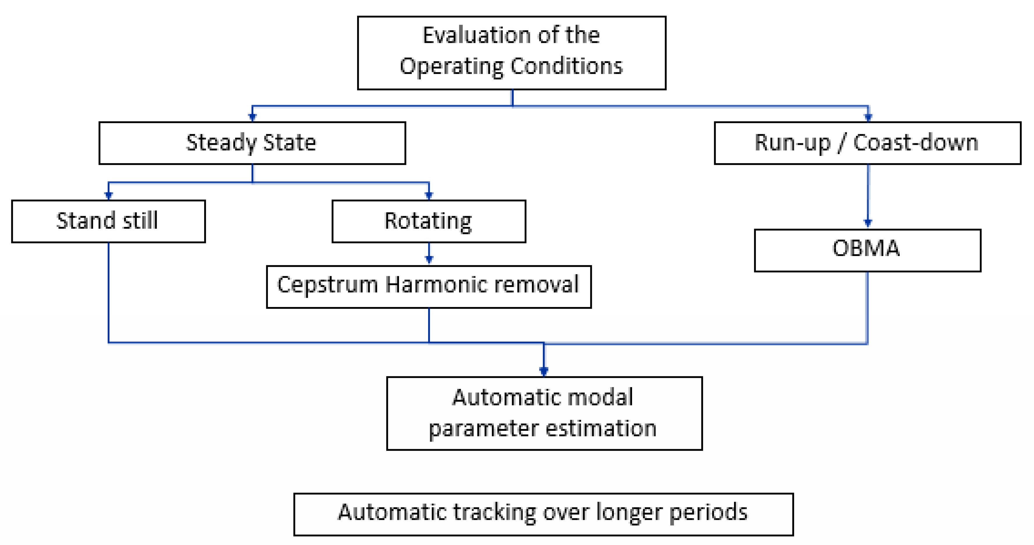
3. Methodology
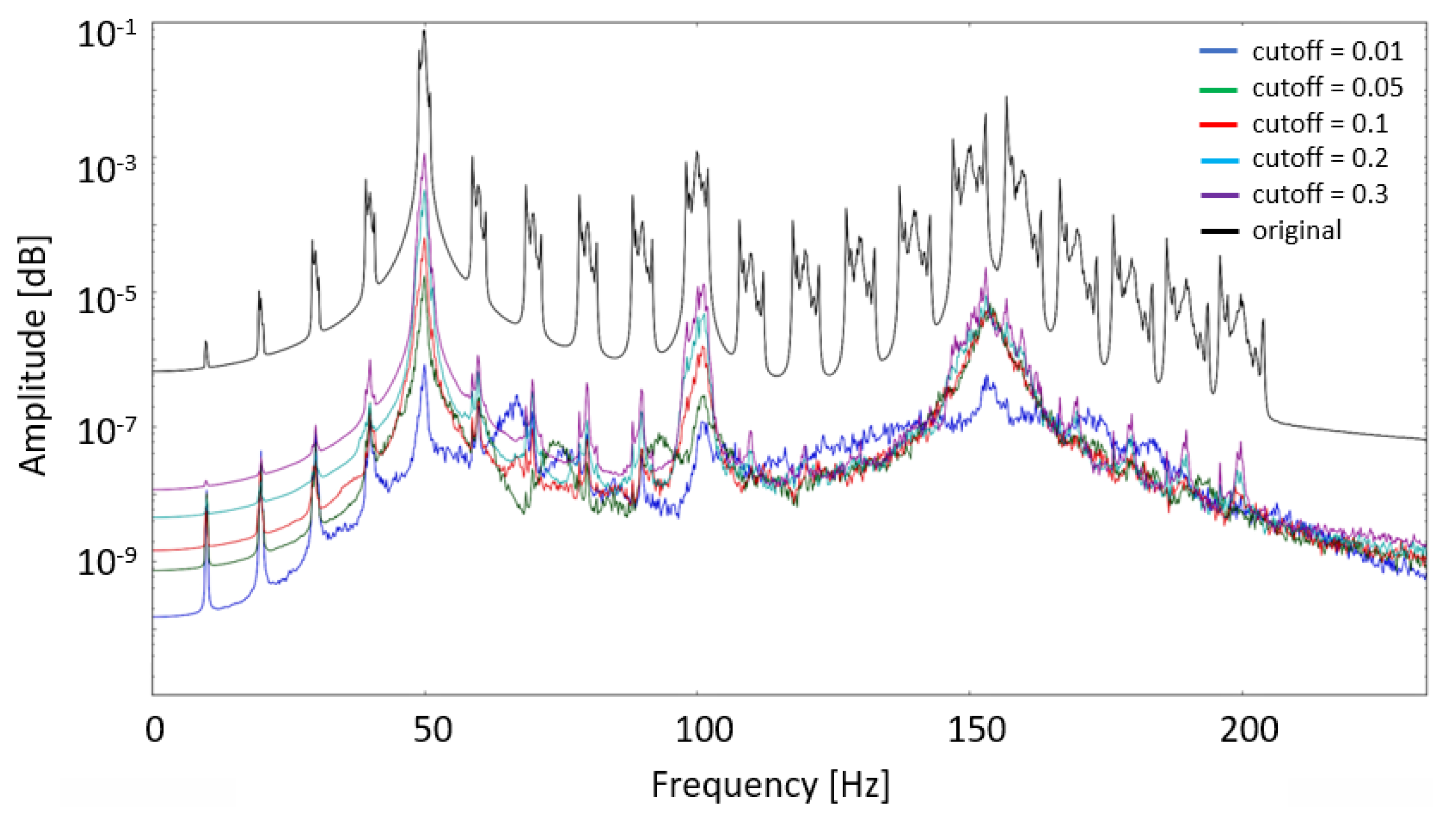
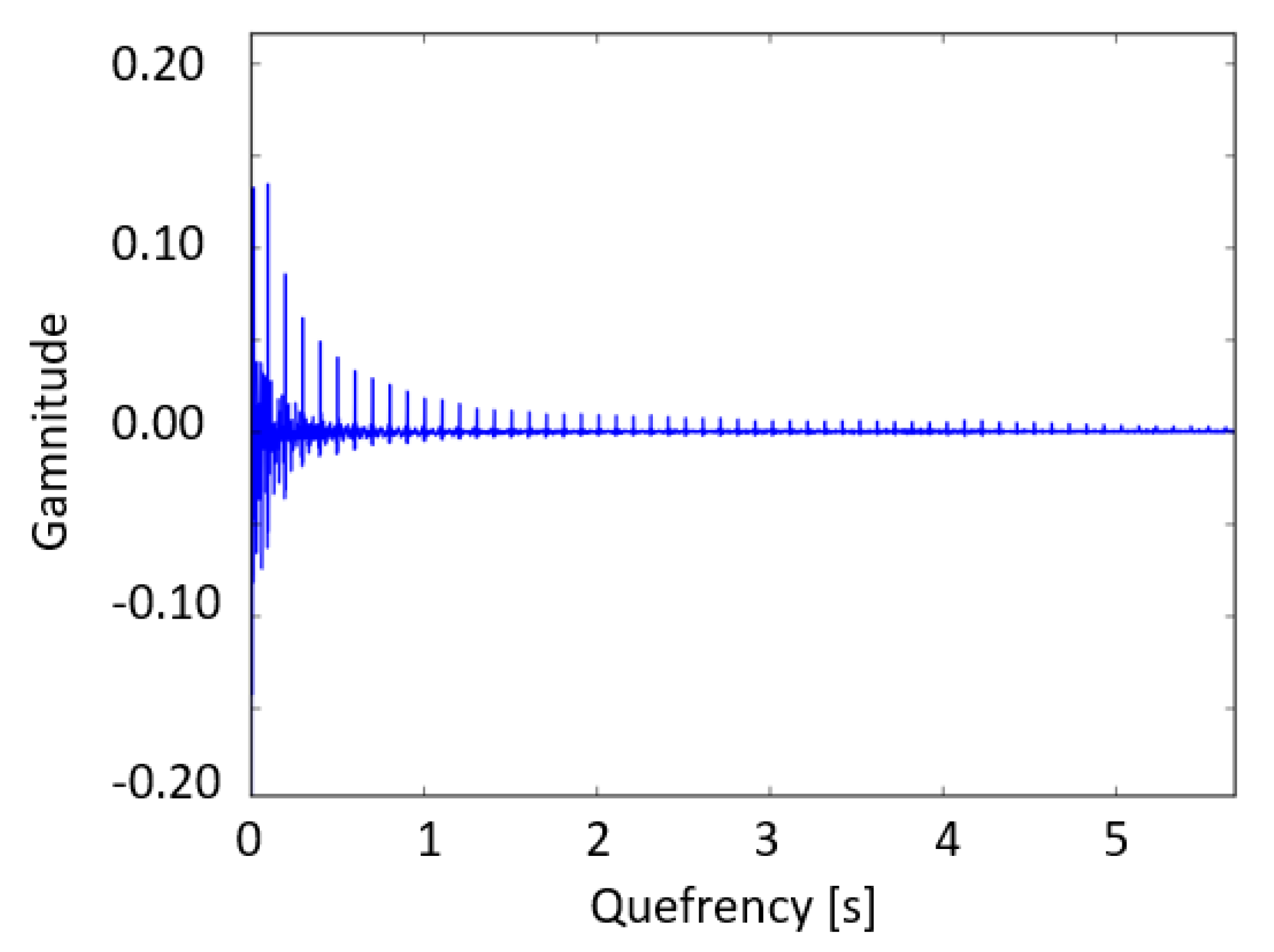
3.1. Selection of the Cepstrum Lifter
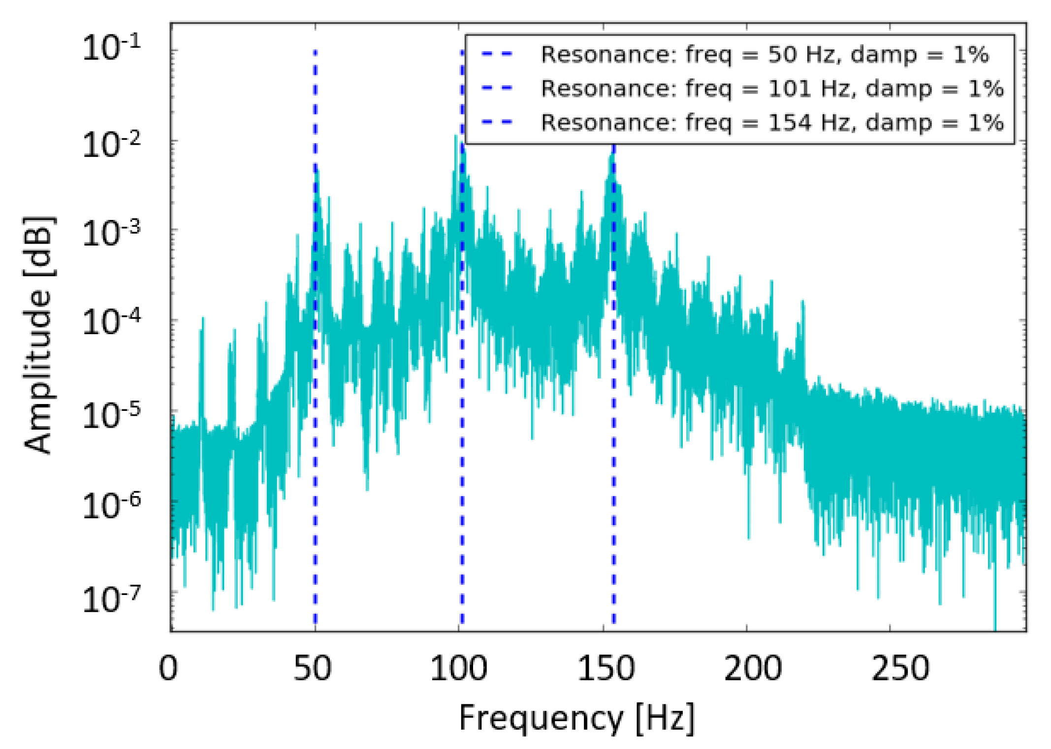
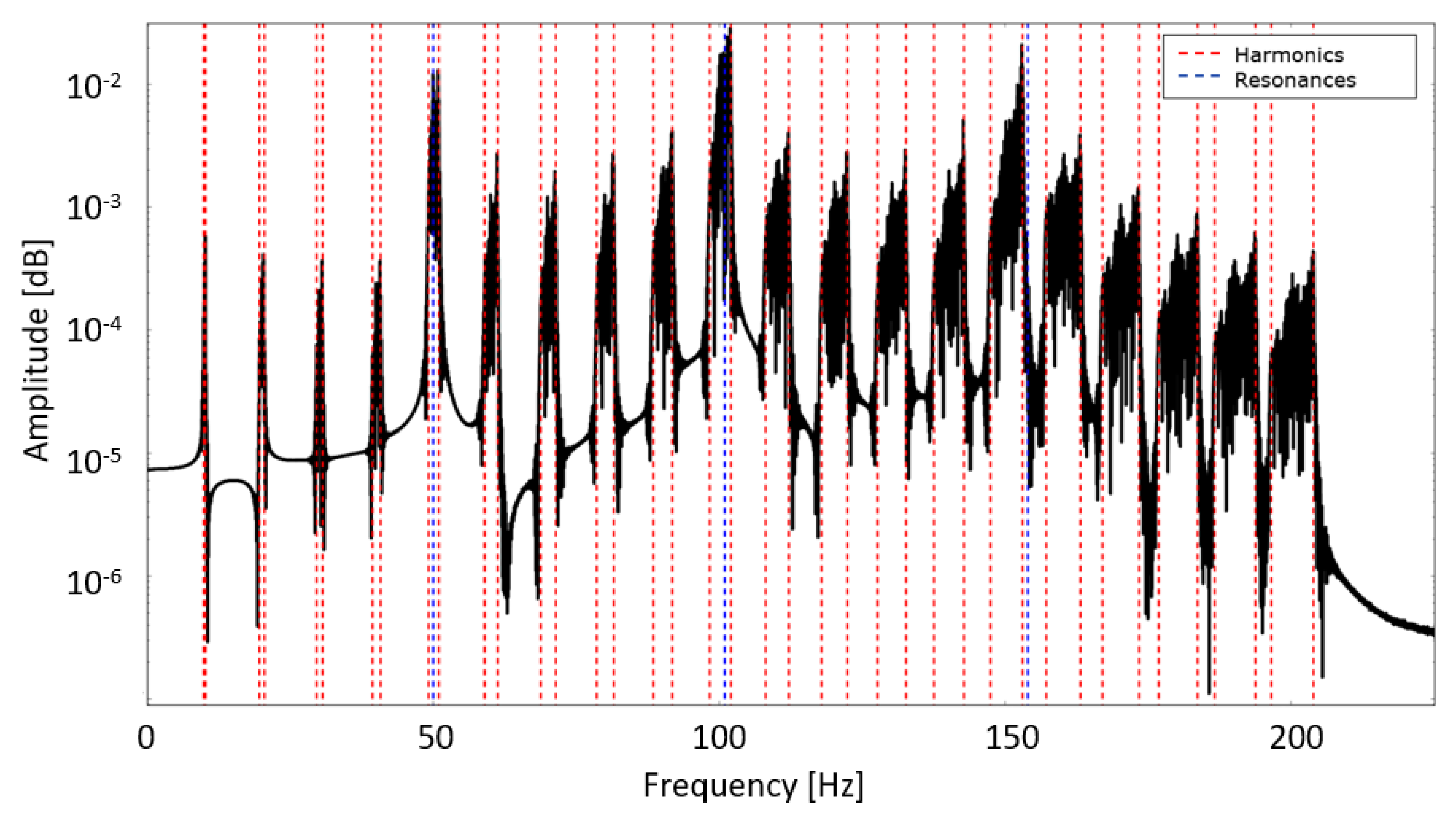
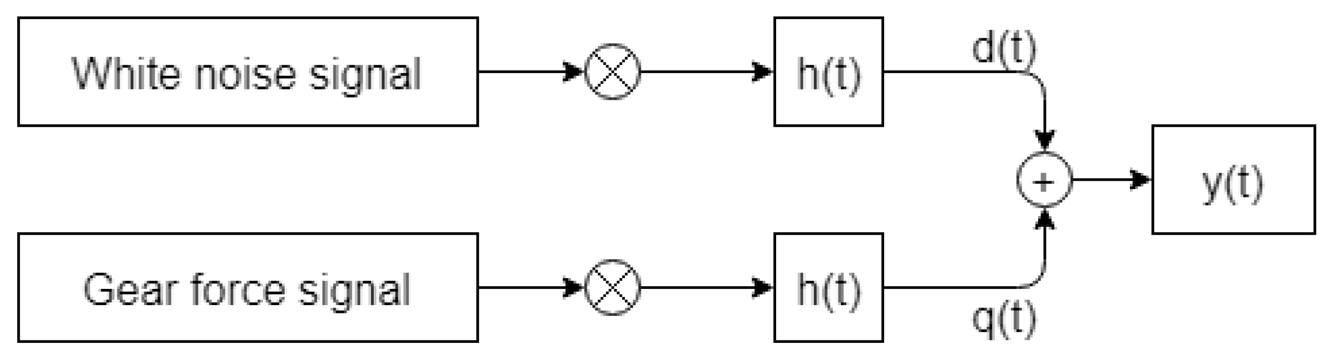
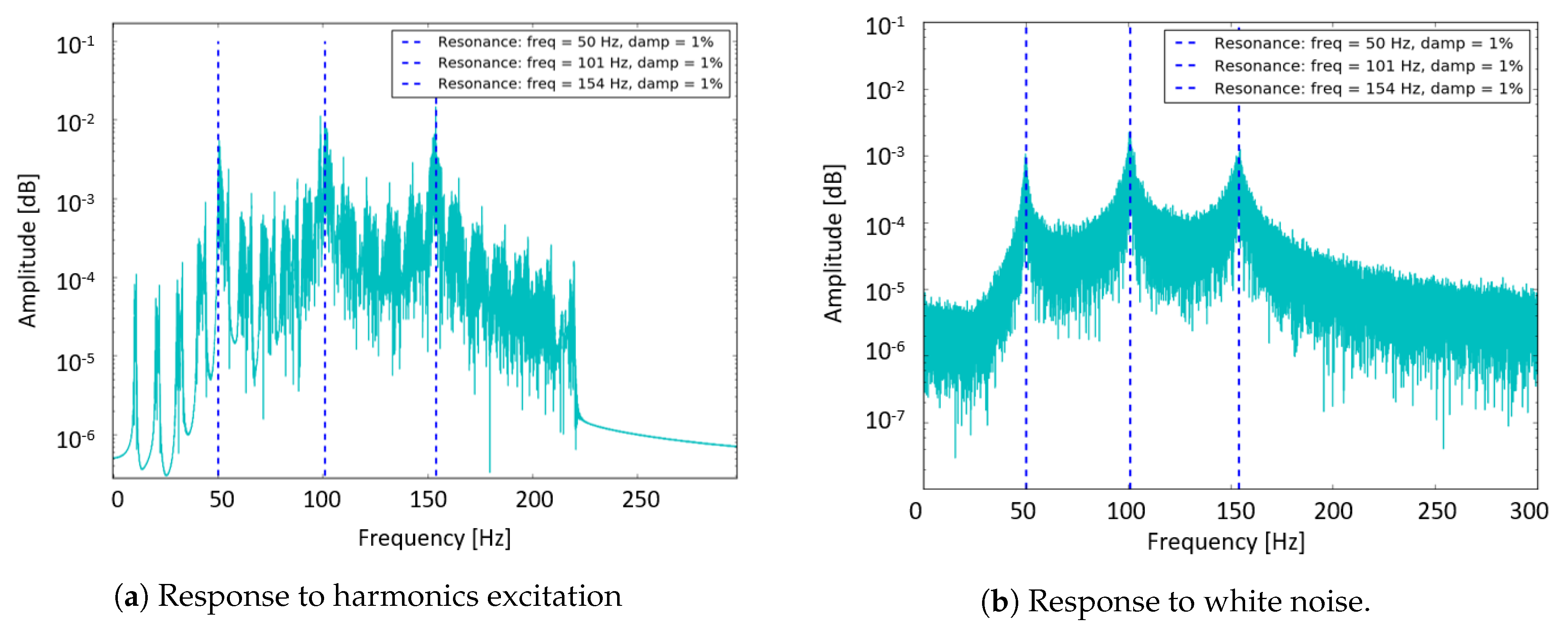
- Gear force signal with 20 harmonics of the fundamental 10 Hz;where N is the number of harmonics, n the harmonic number, the instantaneous amplitude, the instantaneous phase and the rotational speed.
- White noise signal.where is white Gaussian noise normally and independently distributed signal.
3.2. Automatic Selection of the Cutoff Quefrency
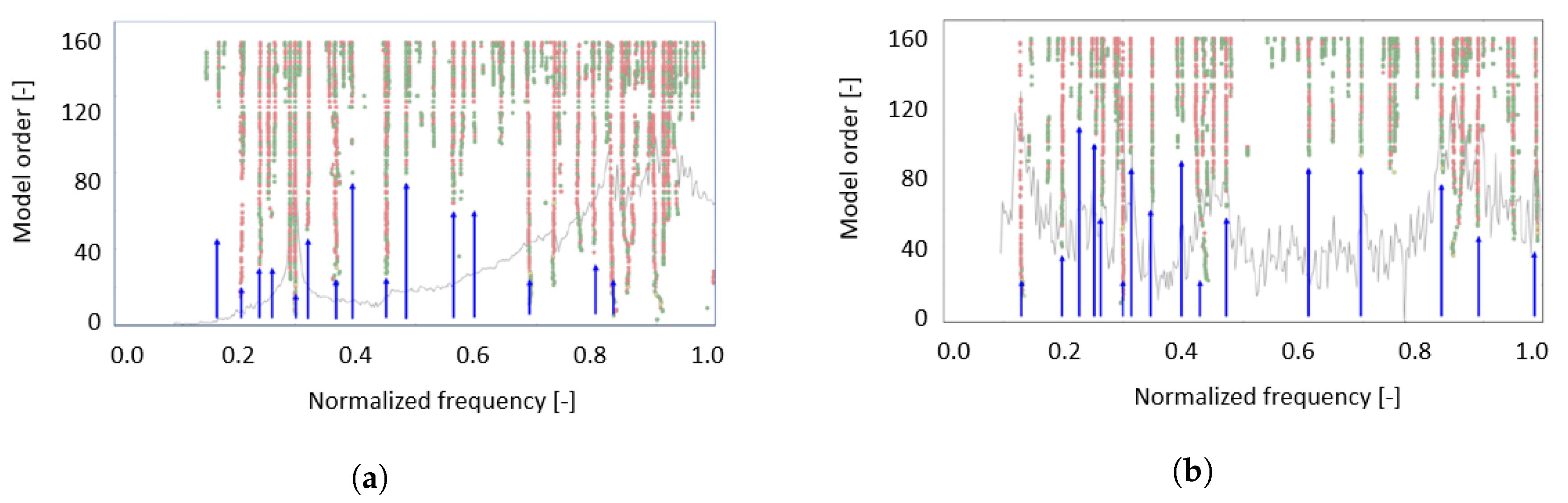
3.3. Automatic Modal Parameter Estimation
- Separation of certainly spurious and possibly physical poles based on single mode validation criteria;
- Grouping the possibly physical poles in separated clusters;
- Selection of the clusters containing physical modes
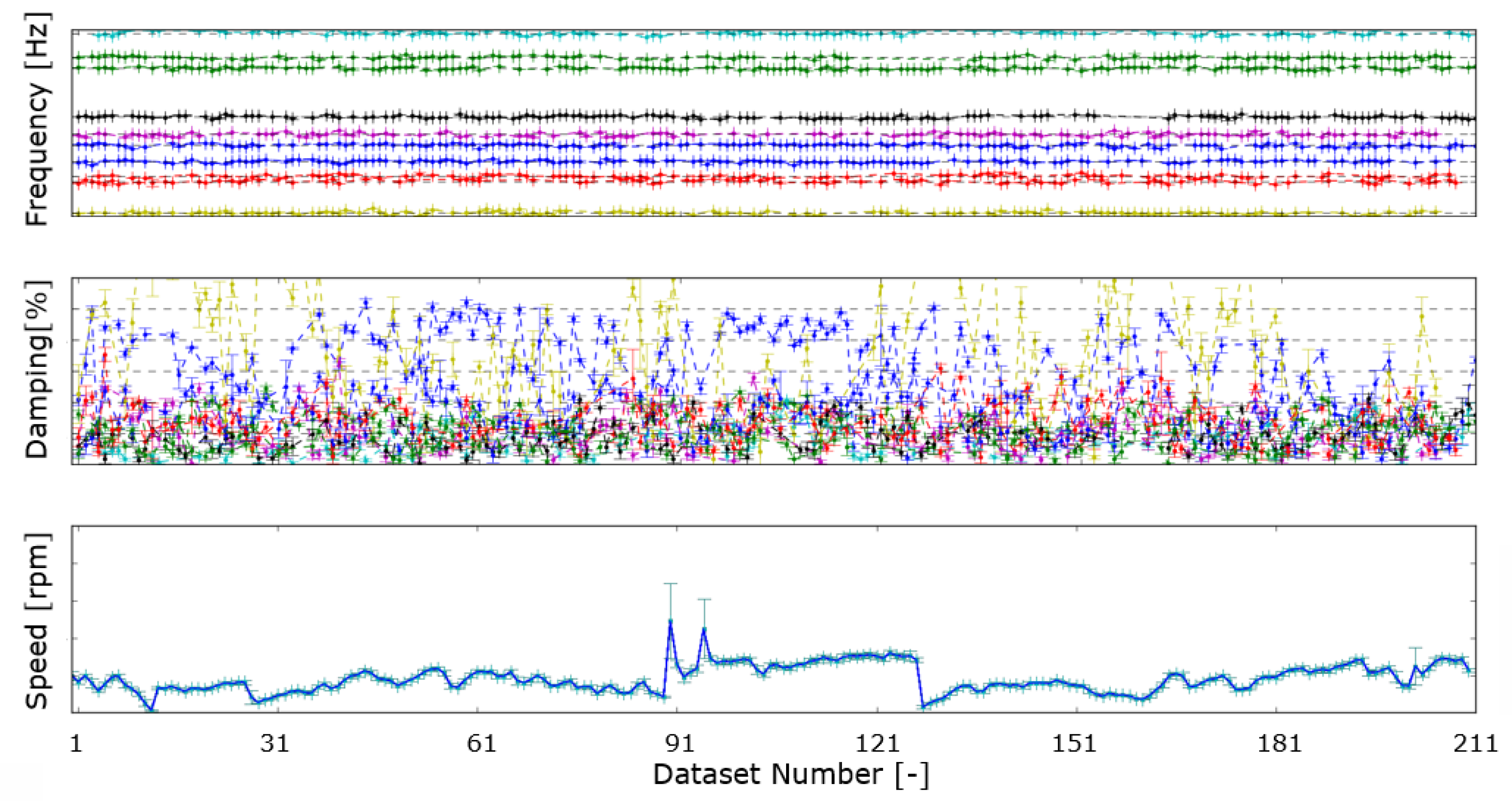
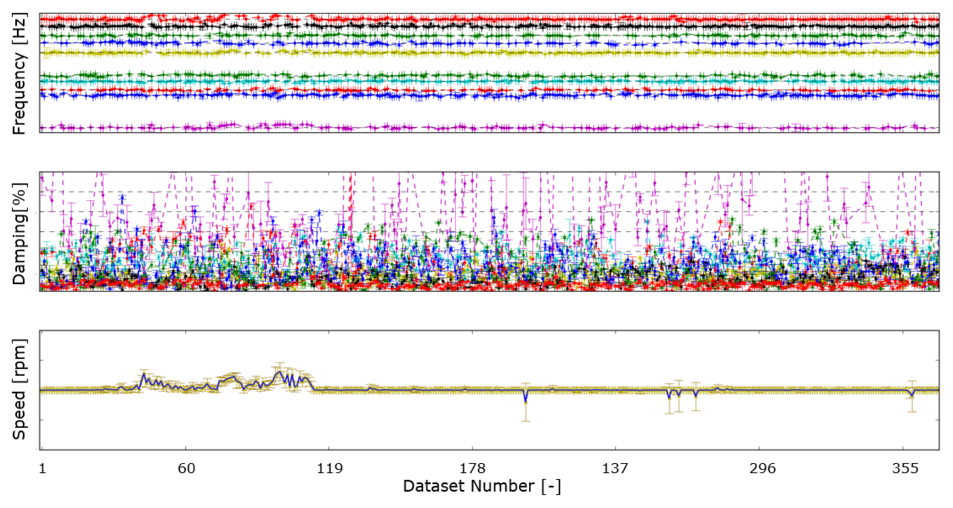
3.4. Automatic Modal Parameters Tracking
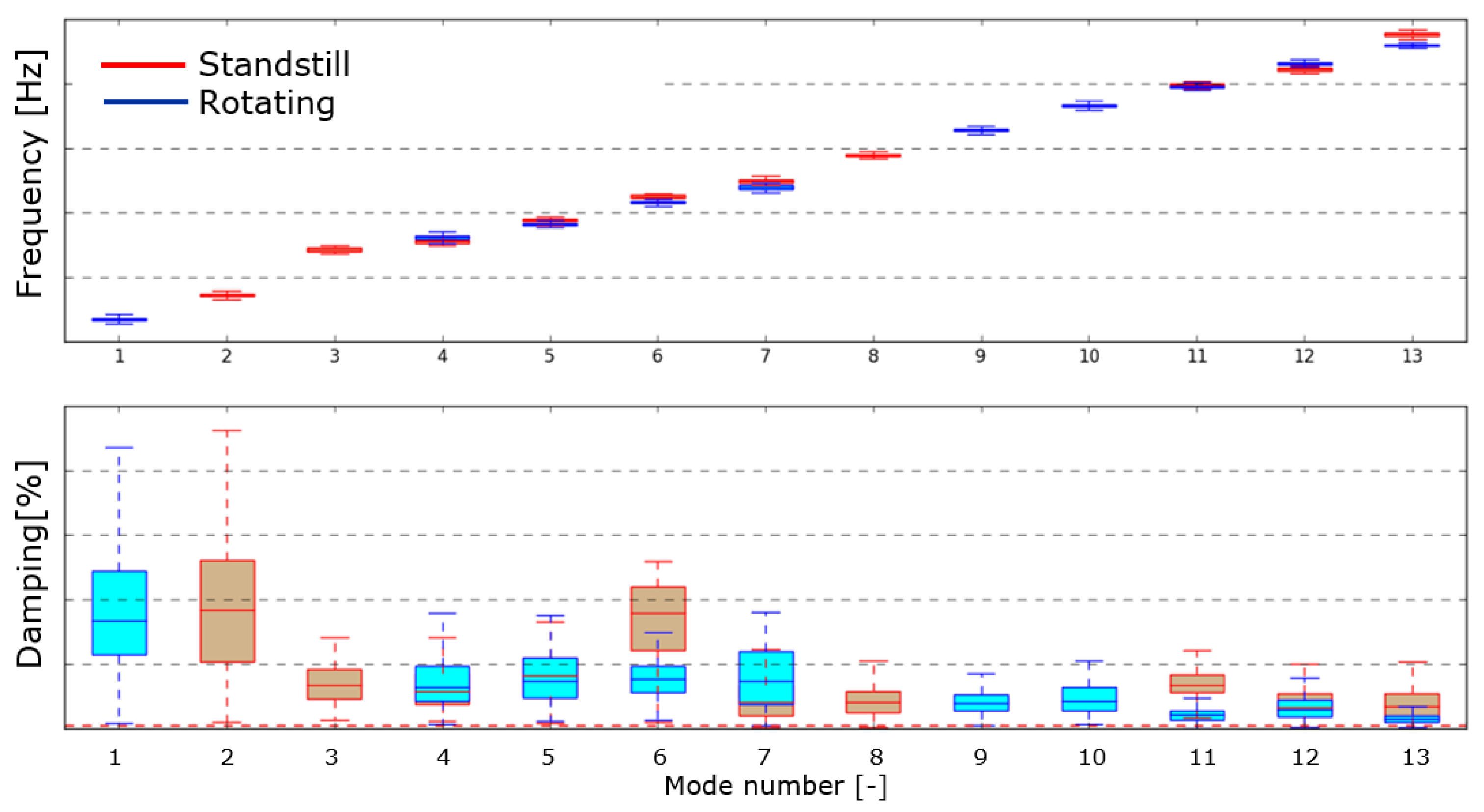
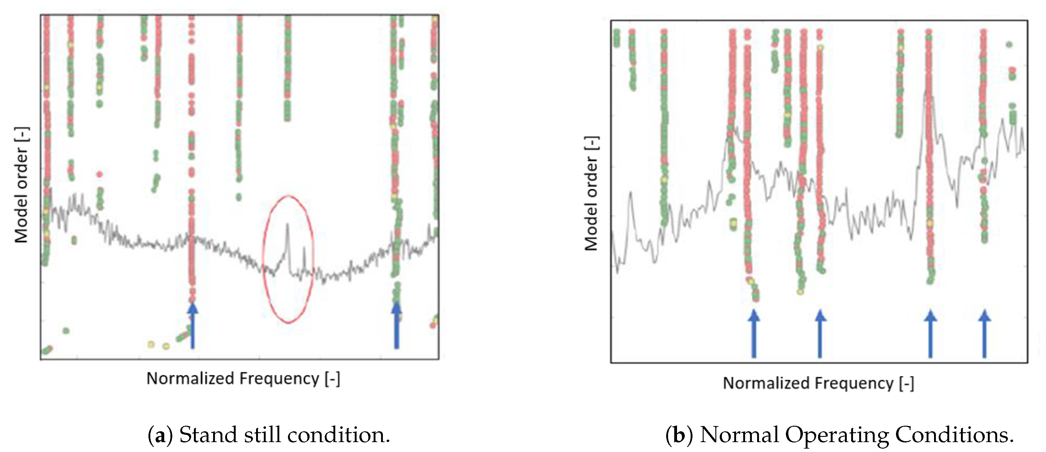
4. Results and Discussion
5. Conclusions
Author Contributions
Funding
Acknowledgments
Conflicts of Interest
Abbreviations
| NVH | Noise, Vibration and Harshness |
| OMA | Operational Modal Analysis |
| pLSCF | poly-reference Least-Squares Complex Frequency-Domain |
| FFT | Fast Fourier Transform |
| MAC | Modal Assurance Criterion |
| SCADA | Supervisory Control and Data Acquisition |
References
- Reynders, E. System identification methods for (operational) modal analysis: review and comparison. Arch. Comput. Methods Eng. 2012, 19, 51–124. [Google Scholar] [CrossRef]
- Schantz, C.; Gerhard, K.; Donnal, J.; Moon, J.; Sievenpiper, B.; Leeb, S.; Thomas, K. Retrofittable machine condition and structural excitation monitoring from the terminal box. IEEE Sens. J. 2016, 16, 1224–1232. [Google Scholar] [CrossRef]
- Vanhollebeke, F. Dynamic Analysis of a Wind Turbine Gearbox Towards Prediction of Mechanical Tonalities. Ph.D. Thesis, KU Leuven, Leuven, Belgium, 2015. [Google Scholar]
- Fowler, K.; Koppen, E. Internal legislation for wind turbine noise. In Proceedings of the EuroNoise 2015, Maastricht, The Netherlands, 31 May–3 June 2015. [Google Scholar]
- Tcherniak, D.; Chauhan, S.; Hansen, M.H. Applicability limits of operational modal analysis to operational wind turbines. In Structural Dynamics and Renewable Energy; Volume 1, Springer: New York, NY, USA, 2011; pp. 317–327. [Google Scholar]
- Weijtjens, W.; Shirzadeh, R.; De Sitter, G.; Devriendt, C. Classifying resonant frequencies and damping values of an offshore wind turbine on a monopile foundation for different operational conditions. In Proceedings of the EWEA, Barcelona, Spain, 10–13 March 2014. [Google Scholar]
- Gade, S.; Schlombs, R.; Hundeck, C.; Fenselau, C. Operational modal analysis on a wind turbine gearbox. In Proceedings of the Conference & Exposition on Structural Dynamics, Orlando, FL, USA, 9–12 February 2009. [Google Scholar]
- Helsen, J.; Vanhollebeke, F.; Vandepitte, D.; Desmet, W. Some trends and challenges in wind turbine upscaling. In Proceedings of the ISMA International Conference on Noise and Vibration, Leuven, Belgium, 17–19 September 2012; p. ID–593. [Google Scholar]
- El-Kafafy, M.; Colanero, L.; Gioia, N.; Devriendt, C.; Guillaume, P.; Helsen, J. Modal Parameters Estimation of an Offshore Wind Turbine Using Measured Acceleration Signals from the Drive Train. In Structural Health Monitoring & Damage Detection; Volume 7, Springer: Cham, Switzerland, 2017; pp. 41–48. [Google Scholar]
- El-Kafafy, M.; Devriendt, C.; Guillaume, P.; Helsen, J. Automatic tracking of the modal parameters of an offshore wind turbine drivetrain system. Energies 2017, 10, 574. [Google Scholar] [CrossRef]
- Randall, R.B. A history of cepstrum analysis and its application to mechanical problems. Mech. Syst. Signal Process. 2017, 97, 3–19. [Google Scholar] [CrossRef]
- Randall, R.; Sawalhi, N.; Coats, M. A comparison of methods for separation of deterministic and random signals. Int. J. Cond. Monit. 2011, 1, 11–19. [Google Scholar] [CrossRef]
- Randall, R.B.; Sawalhi, N. Cepstral removal of periodic spectral components from time signals. In Advances in Condition Monitoring of Machinery in Non-Stationary Operations; Springer: Berlin/Heidelberg, Germany, 2014; pp. 313–324. [Google Scholar]
- Randall, R.B. Cepstral methods of operational modal analysis. Encycl. Struct. Health Monit. 2009. [Google Scholar] [CrossRef]
- Randall, R.; Peeters, B.; Antoni, J.; Manzato, S. New cepstral methods of signal pre-processing for operational modal analysis. In Proceedings of the International Conference on Noise and Vibration Engineering (ISMA), Leuven, Belgium, 17–19 September 2012. [Google Scholar]
- Peeters, C.; Guillaume, P.; Helsen, J. A comparison of cepstral editing methods as signal pre-processing techniques for vibration-based bearing fault detection. Mech. Syst. Signal Process. 2017, 91, 354–381. [Google Scholar] [CrossRef]
- Pintelon, R.; Peeters, B.; Guillaume, P. Continuous-time operational modal analysis in the presence of harmonic disturbances. Mech. Syst. Signal Process. 2008, 22, 1017–1035. [Google Scholar] [CrossRef]
- Di Lorenzo, E.; Manzato, S.; Vanhollebeke, F.; Goris, S.; Peeters, B.; Desmet, W.; Marulo, F. Dynamic characterization of wind turbine gearboxes using Order-Based Modal Analysis. In Proceedings of the International Conference on Noise and Vibration Engineering (Isma2014) and International Conference on Uncertainty in Structural Dynamics (Usd2014), Leuven, Belgium, 15–17 September 2014; pp. 4349–4362. [Google Scholar]
- Bogert, B.P. The quefrency analysis of time series for echoes; Cepstrum, pseudo-autocovariance, cross-cepstrum and saphe cracking. In Time Series Analysis; John Wiley & Sons: Hoboken, NJ, USA, 1963; pp. 209–243. [Google Scholar]
- Randall, R.; Sawalhi, N. Editing time signals using the real cepstrum. In Proceedings of the MFPT Conference, Virginia Beach, VA, USA, 10–12 May 2011. [Google Scholar]
- Roussel, J.; Haritopoulos, M.; Sekko, E.; Capdessus, C.; Antoni, J. Application of Speed Transform to the diagnosis of a roller bearing in variable speed. In Proceedings of the Conference Surveillance, Institute of Technology of Chartres, Chartres, France, 29–30 October 2013; Volume 7, pp. 29–30. [Google Scholar]
- Zhang, L.; Brincker, R. An overview of operational modal analysis: Major development and issues. In Proceedings of the 1st International Operational Modal Analysis Conference, Copenhagen, Denmark, 26–27 April 2005; pp. 179–190. [Google Scholar]
- Peeters, B.; Van der Auweraer, H. PolyMAX: A revolution in operational modal analysis. In Proceedings of the 1st International Operational Modal Analysis Conference, Copenhagen, Denmark, 26–27 April 2005; pp. 26–27. [Google Scholar]
- Oppenheim, A.V.; Schafer, R.W. Digital Signal Processing; Research supported by the Massachusetts Institute of Technology, Bell Telephone Laboratories, and Guggenheim Foundation; Englewood Cliffs, N.J., Ed.; Prentice-Hall, Inc.: Upper Saddle River, NJ, USA, 1975; 598p. [Google Scholar]
- Cauberghe, B. Applied Frequency-Domain System Identification in the Field of Experimental and Operational Modal Analysis. Ph.D. Thesis, Vrije Universiteit Brussel, Brussel, Belgium, 2004. [Google Scholar]
- Randall, R.B.; Coats, M.D.; Smith, W.A. Repressing the effects of variable speed harmonic orders in operational modal analysis. Mech. Syst. Signal Process. 2016, 79, 3–15. [Google Scholar] [CrossRef]
- Peeters, B.; Lau, J.; Lanslot, J.; Auweraer, H.v.d. Automatic modal analysis-Myth or reality? Sound Vib. 2008, 42, 17. [Google Scholar]
- Lanslots, J.; Rodiers, B.; Peeters, B. Automated pole-selection: Proof-of-concept and validation. In Proceedings of the ISMA International Conference on Noise and Vibration Engineering, Leuven, Belgium, 20–22 September 2004. [Google Scholar]
- Magalhaes, F.; Cunha, A.; Caetano, E. Online automatic identification of the modal parameters of a long span arch bridge. Mech. Syst. Signal Process. 2009, 23, 316–329. [Google Scholar] [CrossRef]
- Chauhan, S.; Tcherniak, D. Clustering approaches to automatic modal parameter estimation. In Proceedings of the International Modal Analysis Conference (IMAC), Orlando, FL, USA, 9–12 February 2009. [Google Scholar]
- Goethals, I.; Vanluyten, B.; De Moor, B. Reliable spurious mode rejection using self learning algorithms. In Proceedings of the International Conference on Noise and Vibration Engineering (ISMA 2004), Leuven, Belgium, 20–22 September 2004; pp. 991–1003. [Google Scholar]
- Devriendt, C.; Elkafafy, M.; De Sitter, G.; Guillaume, P. Continuous dynamic monitoring of an offshore wind turbine on a monopile foundation. In Proceedings of the ISMA2012, Leuven, Belgium, 17–19 September 2012. [Google Scholar]
- Reynders, E.; Houbrechts, J.; De Roeck, G. Fully automated (operational) modal analysis. Mech. Syst. Signal Process. 2012, 29, 228–250. [Google Scholar] [CrossRef]


| Natural Frequency (Hz) | Damping Ratio (%) | |
|---|---|---|
| Mode 1 | 50 | 1 |
| Mode 2 | 101 | 1 |
| Mode 3 | 154 | 1 |
| Time Exponential | Angle Exponential | Time Rectangular | Angle Rectangular | |||||
|---|---|---|---|---|---|---|---|---|
| Freq (Hz) | Damp (%) | Freq (Hz) | Damp (%) | Freq (Hz) | Damp (%) | Freq (Hz) | Damp (%) | |
| Estimated | Corrected | |||||||
| Cutoff Quefrency = 0.05 | ||||||||
| 50.21 | 6.49 | 0.16 | 49.78 | 5.2 | 48.73 | 2.31 | 49.97 | 0.91 |
| 100.82 | 3.93 | 0.77 | 101.32 | 0.99 | 102.56 | 1.31 | 101.43 | 1.12 |
| 154.26 | 2.95 | 0.9 | 153.92 | 2.41 | 156.01 | 0.97 | 154.00 | 1.13 |
| Cutoff Quefrency = 0.1 | ||||||||
| 50.06 | 2.63 | −0.54 | 49.94 | 2.74 | 49.86 | 1.05 | 50.02 | 0.95 |
| 100.38 | 1.93 | 0.34 | 100.88 | 1.88 | 100.72 | 0.94 | 100.92 | 0.98 |
| 154.693 | 1.86 | 0.83 | 153.98 | 1.73 | 153.56 | 1.07 | 153.99 | 1.05 |
| Cutoff Quefrency = 0.2 | ||||||||
| 49.96 | 0.89 | −0.7 | 49.99 | 1.66 | 50.00 | 0.08 | 49.99 | 0.90 |
| 100.31 | 0.93 | −0.13 | 100.99 | 1.24 | 100.52 | 0.27 | 100.99 | 0.95 |
| 154.20 | 1.09 | 0.58 | 153.88 | 1.34 | 153.50 | 0.18 | 153.86 | 0.99 |
| Time Exponential | Angle Exponential | Time Rectangular | Angle Rectangular | |||||
|---|---|---|---|---|---|---|---|---|
| Freq (Hz) | Damp (%) | Freq (Hz) | Damp (%) | Freq (Hz) | Damp (%) | Freq (Hz) | Damp (%) | |
| Estimated | Corrected | |||||||
| Cutoff Quefrency = 0.05 | ||||||||
| 50.20 | 6.70 | 0.35 | 49.83 | 4.28 | 47.67 | 3.07 | 49.93 | 1.41 |
| 101.38 | 3.96 | 0.82 | 101.16 | 2.54 | 101.69 | 1.61 | 100.92 | 1.16 |
| 154.30 | 2.96 | 0.89 | 153.89 | 2.10 | 155.06 | 1.60 | 153.91 | 1.15 |
| Cutoff Quefrency = 0.1 | ||||||||
| 50.54 | 3.09 | −0.05 | 49.92 | 2.36 | 50.95 | 0.88 | 49.91 | 0.97 |
| 101.17 | 2.38 | 0.80 | 101.10 | 1.60 | 101.20 | 1.08 | 101.02 | 1.05 |
| 153.99 | 1.74 | 0.72 | 153.99 | 1.56 | 153.92 | 0.72 | 153.99 | 1.10 |
| Cutoff Quefrency = 0.2 | ||||||||
| 50.20 | 4.70 | 3.52 | 49.82 | 4.28 | 50.72 | 0.45 | 49.87 | 0.9 |
| 101.38 | 3.96 | 2.39 | 101.17 | 2.54 | 101.44 | 0.78 | 101.08 | 0.99 |
| 154.30 | 2.96 | 1.94 | 153.86 | 2.10 | 153.90 | 0.44 | 154.07 | 0.99 |
| Time Exponential | Angle Exponential | Time Rectangular | Angle Rectangular | |||||
|---|---|---|---|---|---|---|---|---|
| Freq (Hz) | Damp (%) | Freq (Hz) | Damp (%) | Freq (Hz) | Damp (%) | Freq (Hz) | Damp (%) | |
| Estimated | Corrected | |||||||
| Cutoff Quefrency = 0.05 | ||||||||
| 50.51 | 6.9 | 0.60 | 49.65 | 4.54 | 48.64 | 3.48 | 50.10 | 0.99 |
| 100.67 | 4.30 | 1.13 | 100.96 | 2.40 | 100.51 | 1.12 | 100.89 | 1.07 |
| 154.32 | 2.68 | 0.65 | 154.08 | 1.84 | 155.87 | 1.32 | 154.30 | 1.04 |
| Cutoff Quefrency = 0.1 | ||||||||
| 49.82 | 3.12 | −0.07 | 49.72 | 2.01 | 50.35 | 0.09 | 50.07 | 0.94 |
| 100.54 | 2.90 | 1.32 | 101.05 | 1.62 | 100.58 | 0.36 | 101.11 | 0.99 |
| 14.16 | 1.70 | 0.60 | 154.08 | 1.43 | 154.17 | 0.64 | 154.77 | 1.05 |
| Cutoff Quefrency = 0.2 | ||||||||
| 49.54 | 1.73 | 0.13 | 49.91 | 1.15 | 49.41 | 0.66 | 49.96 | 0.91 |
| 100.55 | 2.00 | 1.20 | 100.91 | 1.30 | 100.48 | 1.50 | 100.90 | 0.94 |
| 154.13 | 1.15 | 0.63 | 154.03 | 1.25 | 154.03 | 0.64 | 154.00 | 0.98 |
| (a) | (b) | ||
|---|---|---|---|
| Frequency (-) | Damping (%) | Frequency (-) | Damping (%) |
| - | - | 0.14 | 1.19 |
| 0.17 | 0.15 | 0.18 | 0.13 |
| 0.22 | 0.66 | 0.22 | 0.10 |
| 0.24 | 0.25 | 0.24 | 0.12 |
| 0.27 | 0.16 | 0.26 | 0.11 |
| 0.30 | 0.20 | 0.30 | 0.62 |
| 0.32 | 0.29 | 0.32 | 0.18 |
| 0.35 | 0.30 | 0.35 | 0.11 |
| 0.38 | 0.11 | 0.39 | 0.37 |
| 0.45 | 0.30 | 0.45 | 0.18 |
| 0.48 | 0.06 | 0.48 | 0.17 |
| 0.56 | 0.24 | - | - |
| 0.60 | 0.16 | - | - |
| - | - | 0.62 | 0.18 |
| 0.69 | 0.40 | 0.69 | 0.17 |
| 0.80 | 0.18 | 0.79 | 0.12 |
| 0.82 | 0.02 | 0.83 | 0.28 |
| - | - | 0.89 | 0.2 |
| - | - | 0.99 | 0.12 |
© 2019 by the authors. Licensee MDPI, Basel, Switzerland. This article is an open access article distributed under the terms and conditions of the Creative Commons Attribution (CC BY) license (http://creativecommons.org/licenses/by/4.0/).
Share and Cite
Gioia, N.; Peeters, C.; Guillaume, P.; Helsen, J. Identification of Noise, Vibration and Harshness Behavior of Wind Turbine Drivetrain under Different Operating Conditions. Energies 2019, 12, 3401. https://doi.org/10.3390/en12173401
Gioia N, Peeters C, Guillaume P, Helsen J. Identification of Noise, Vibration and Harshness Behavior of Wind Turbine Drivetrain under Different Operating Conditions. Energies. 2019; 12(17):3401. https://doi.org/10.3390/en12173401
Chicago/Turabian StyleGioia, Nicoletta, Cédric Peeters, Patrick Guillaume, and Jan Helsen. 2019. "Identification of Noise, Vibration and Harshness Behavior of Wind Turbine Drivetrain under Different Operating Conditions" Energies 12, no. 17: 3401. https://doi.org/10.3390/en12173401
APA StyleGioia, N., Peeters, C., Guillaume, P., & Helsen, J. (2019). Identification of Noise, Vibration and Harshness Behavior of Wind Turbine Drivetrain under Different Operating Conditions. Energies, 12(17), 3401. https://doi.org/10.3390/en12173401