Backbone—An Adaptable Energy Systems Modelling Framework

 , , , , ,
Abstract

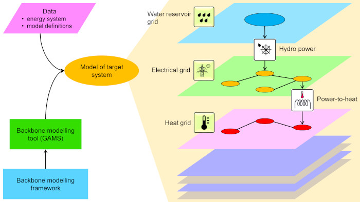
1. Introduction
2. Model Structure Description
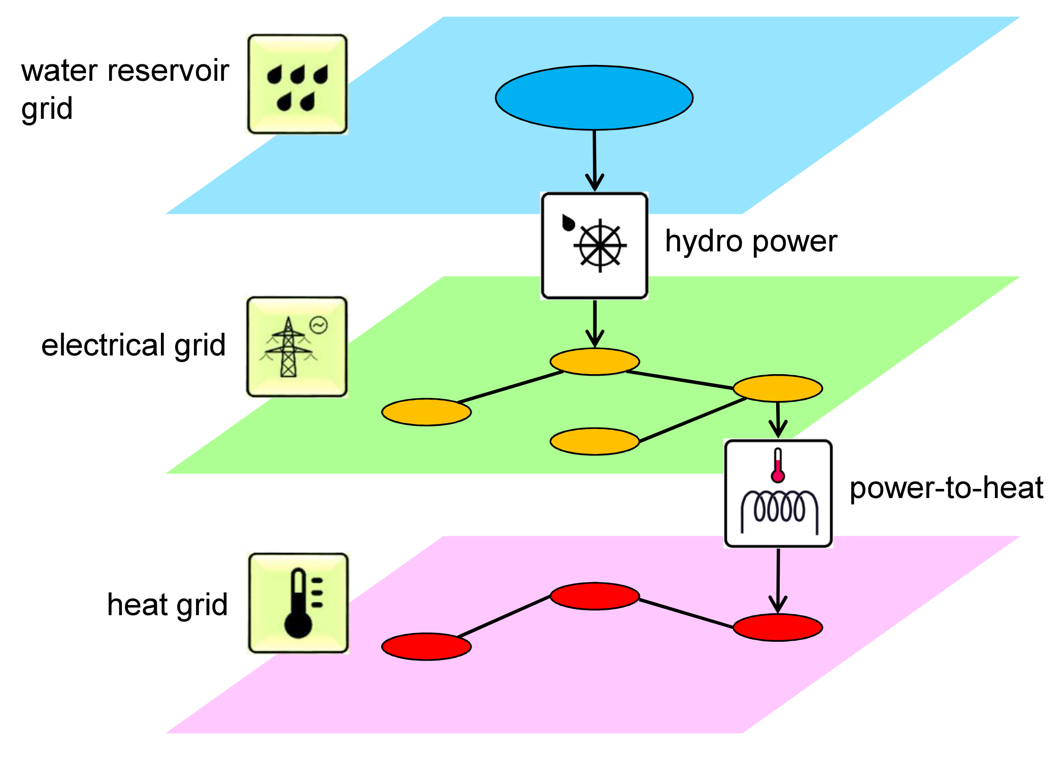
2.1. Network Structure
2.1.1. Grids
2.1.2. Nodes
- State: for example, the energy content, the temperature or similar quantity of the node. Each node can either have a single state, for example, used for storing energy or no state at all.
- –
- Various boundary conditions can be imposed on the state of a node, ranging from simple absolute upper and lower bounds to “softer” bounds that can be exceeded, at the cost of a separately defined penalty. These bounds can be set to be invariant or to follow some pre-determined time series. It is also possible to constrain a state of a node relative to the state of another node.
- Reserve requirements: Just as the energy balance is enforced on the nodal level, so are the possible requirements for operating reserves, explained in more detail in Section 2.4. Reserve requirements are specific to power systems and are unlikely to be directly relevant for other grid types.
- Spill capability: Nodes can be permitted to spill energy, transferring it outside the model boundaries.
- Contain units: Even though units represent a separate entity altogether, each unit must be connected to at least one node.
2.1.3. Lines
- Transfer: Nodes can be connected to other nodes in the same grid via a controlled transfer, which can be defined either as uni- or bi-directional. Naturally, boundaries on the transfer capabilities of nodes can be imposed using various parameters.
- Diffusion: Nodes can be connected to other nodes in the same grid via diffusion coefficients, causing energy to uncontrollably leak from one node to another, depending on the states of said nodes. While diffusion coefficients can technically be defined even for nodes without states, they will have no effect (non-existent states contain zero energy).
- –
- Diffusion can be defined to be asymmetric, resulting in a unidirectional uncontrolled flow of energy from one node to another.
- –
- Self-discharge of energy from individual nodes to outside the model scope is also possible using a separate parameter.
2.1.4. Units
- Production and consumption of energy: A unit can produce energy at a node or consume it.
- –
- While units could be defined to produce energy out of thin air, more often it is the case that the produced energy is defined to increase the consumption of defined fuels (which should have a cost attributed to them) or have limited production capabilities based on time series data (e.g., solar, wind, hydro).
- –
- Consumption of energy in units is treated as “negative production”. Unless some form of energy conversion is defined for the unit in question, the consumed energy is transferred out of the model.
- –
- While nodes could be used to emulate some of the functionality of the units, units provide parameters capable of defining the way in which energy production and consumption function in much more detail.
- Conversion of energy between grids: While energy can diffuse and be transferred between nodes within each grid, units are the only way of transferring (referred to as conversion) energy between nodes in different grids.
- –
- This functionality essentially means that a unit can be connected to multiple nodes and the energy production and consumption variables in each node are linked to each other according to desired conversion rules and constraints.
2.1.5. Resulting Spatial Structure
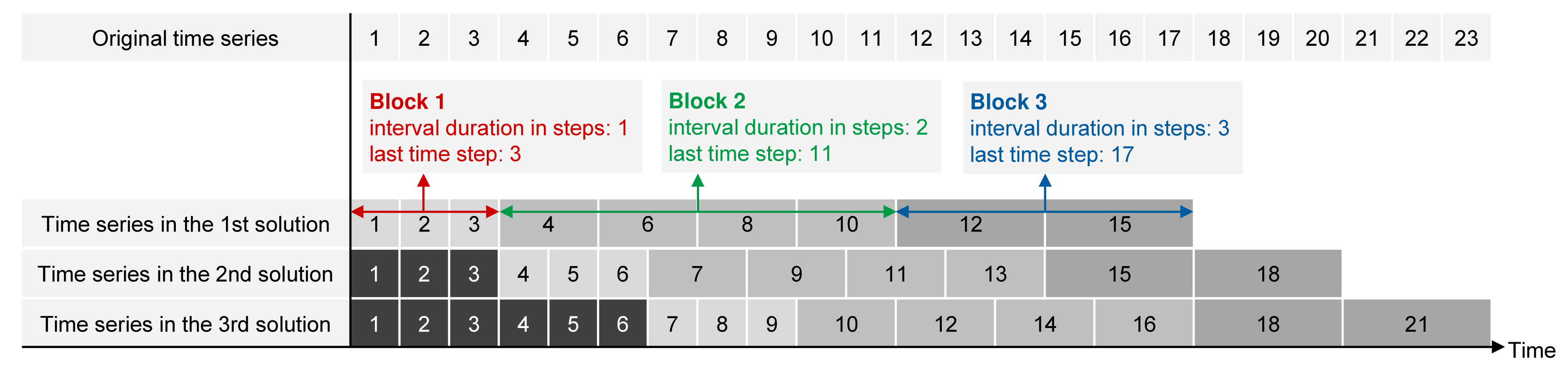
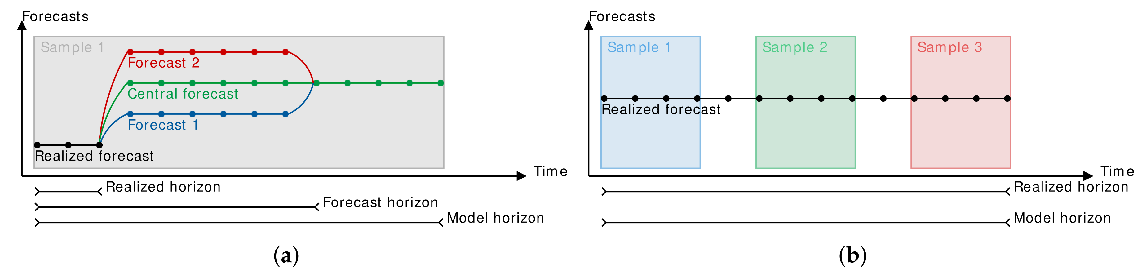
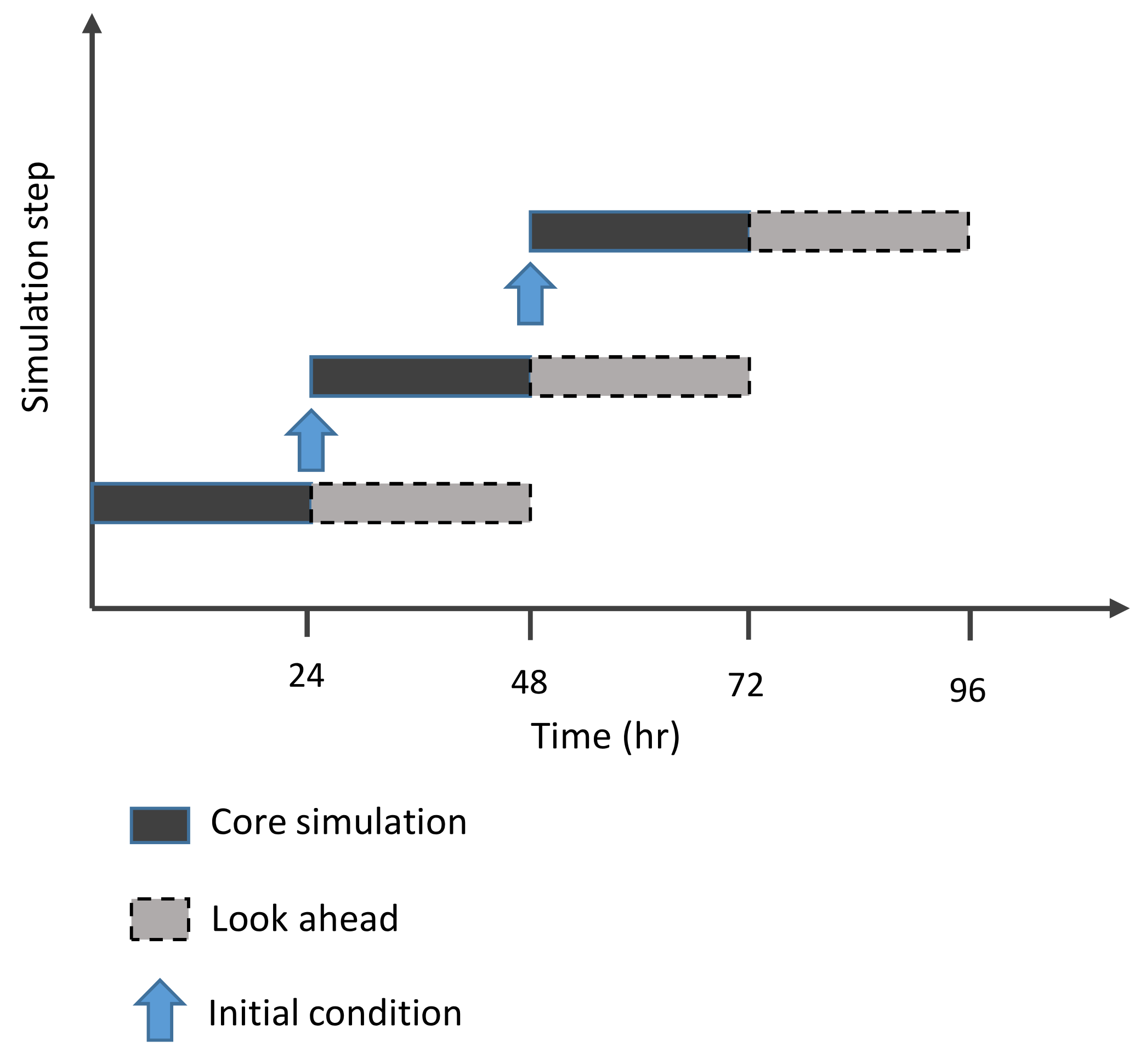
2.2. Temporal Structure
2.3. Technological Structure
2.4. Ancillary Services and Policy Constraints
3. Model Formulation
3.1. Objective
3.2. Energy Balance
3.3. Unit Operation
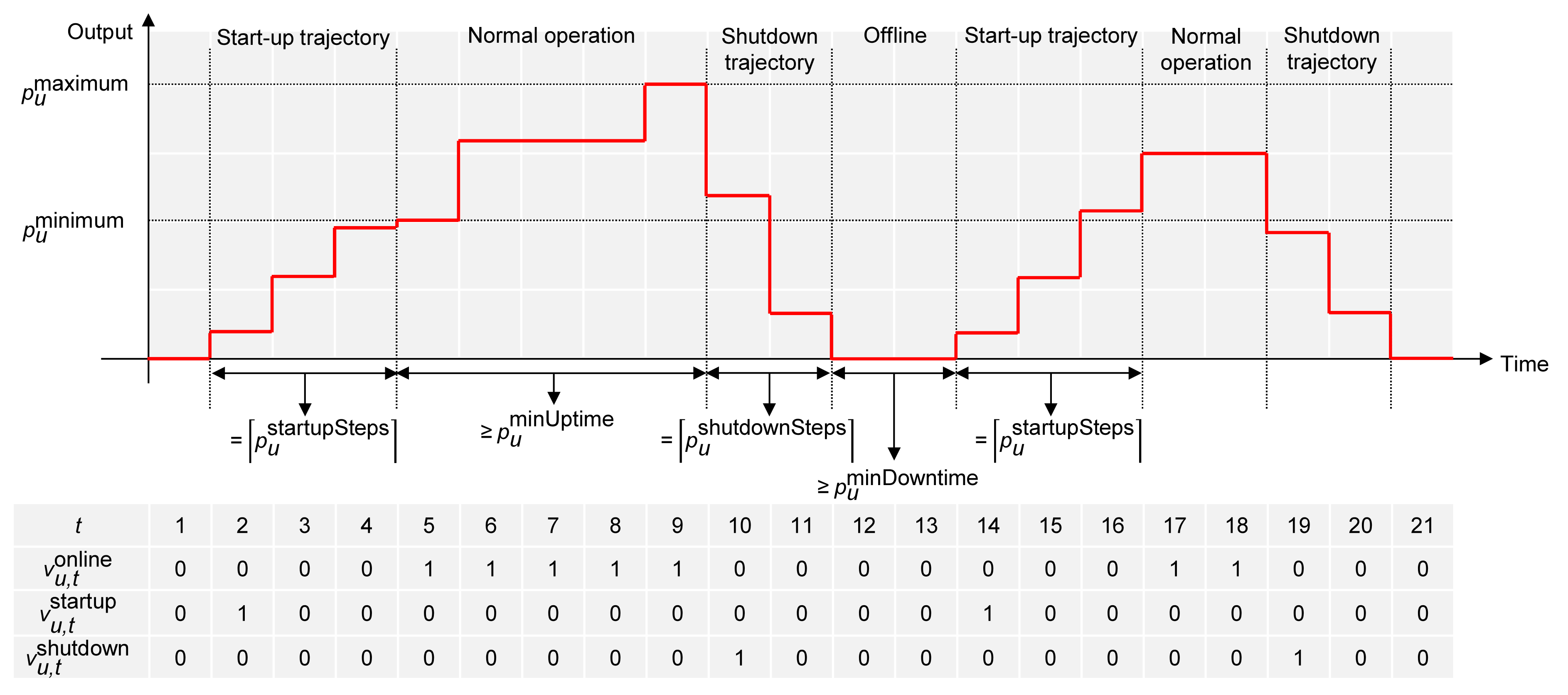
3.3.1. Start-Up and Shutdown
3.3.2. Ramping
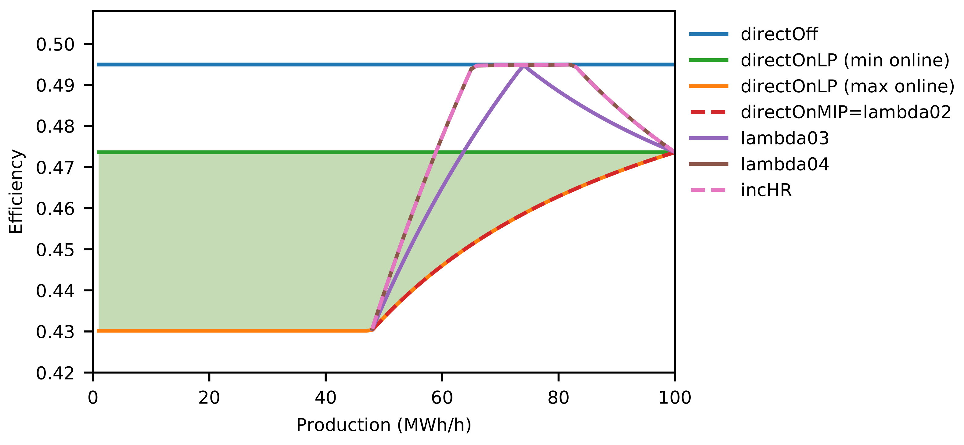
3.3.3. Efficiency
3.3.4. Other Constraints
3.4. Transfers
3.5. System Operation
3.6. Portfolio Design
4. Case Study
4.1. Backbone Modelling Tool
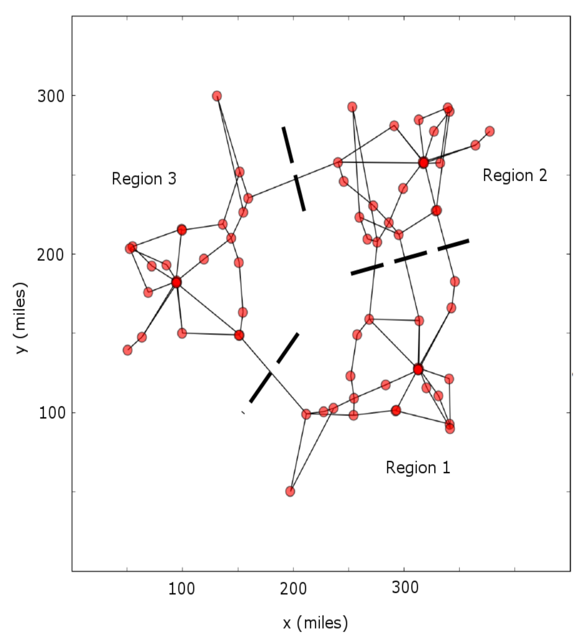
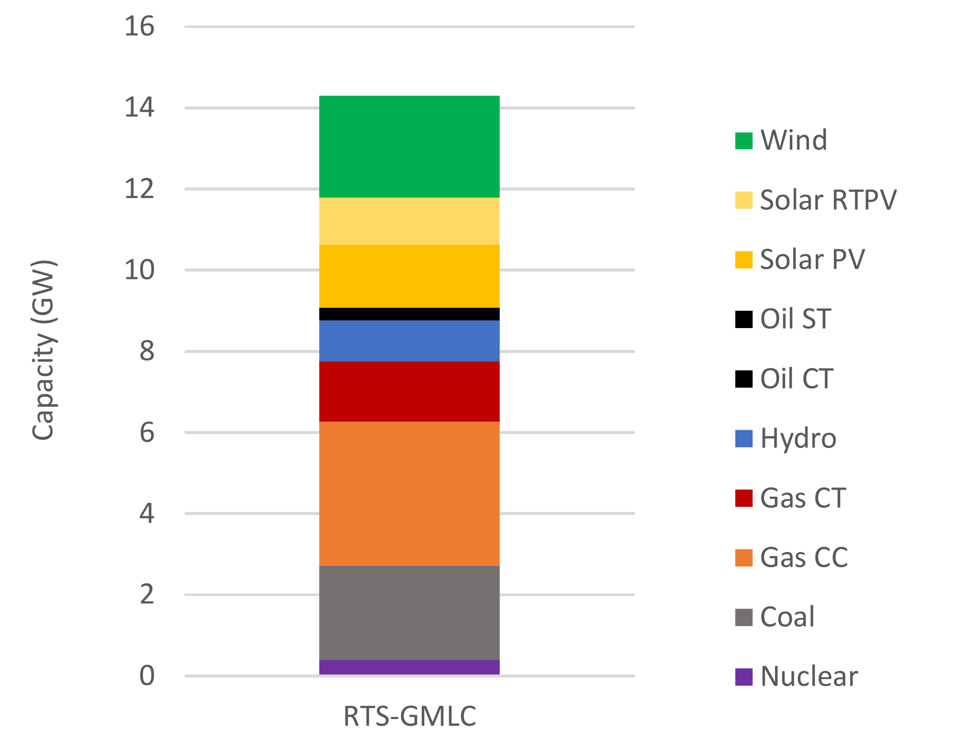
4.2. The RTS-GMLC Test System
4.3. PLEXOS Implementation
4.4. Backbone Implementation
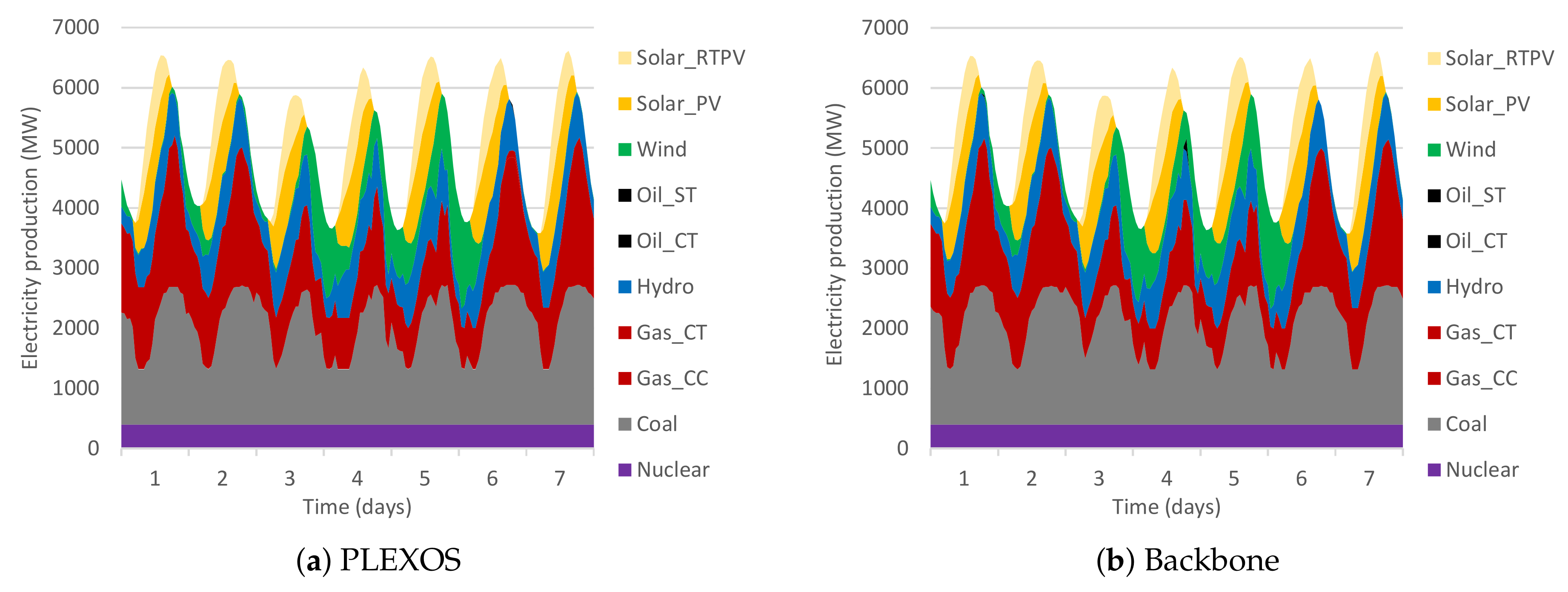
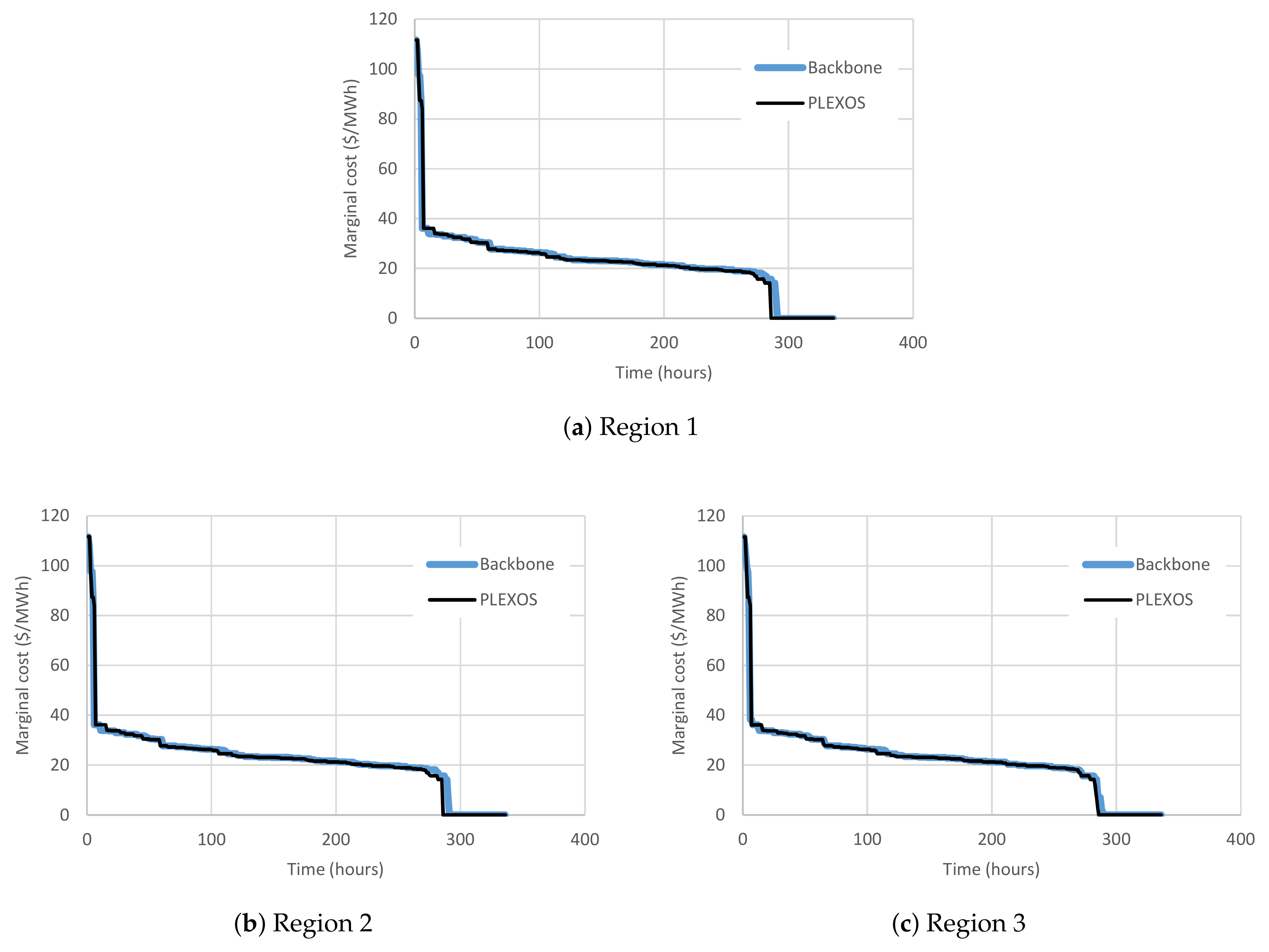
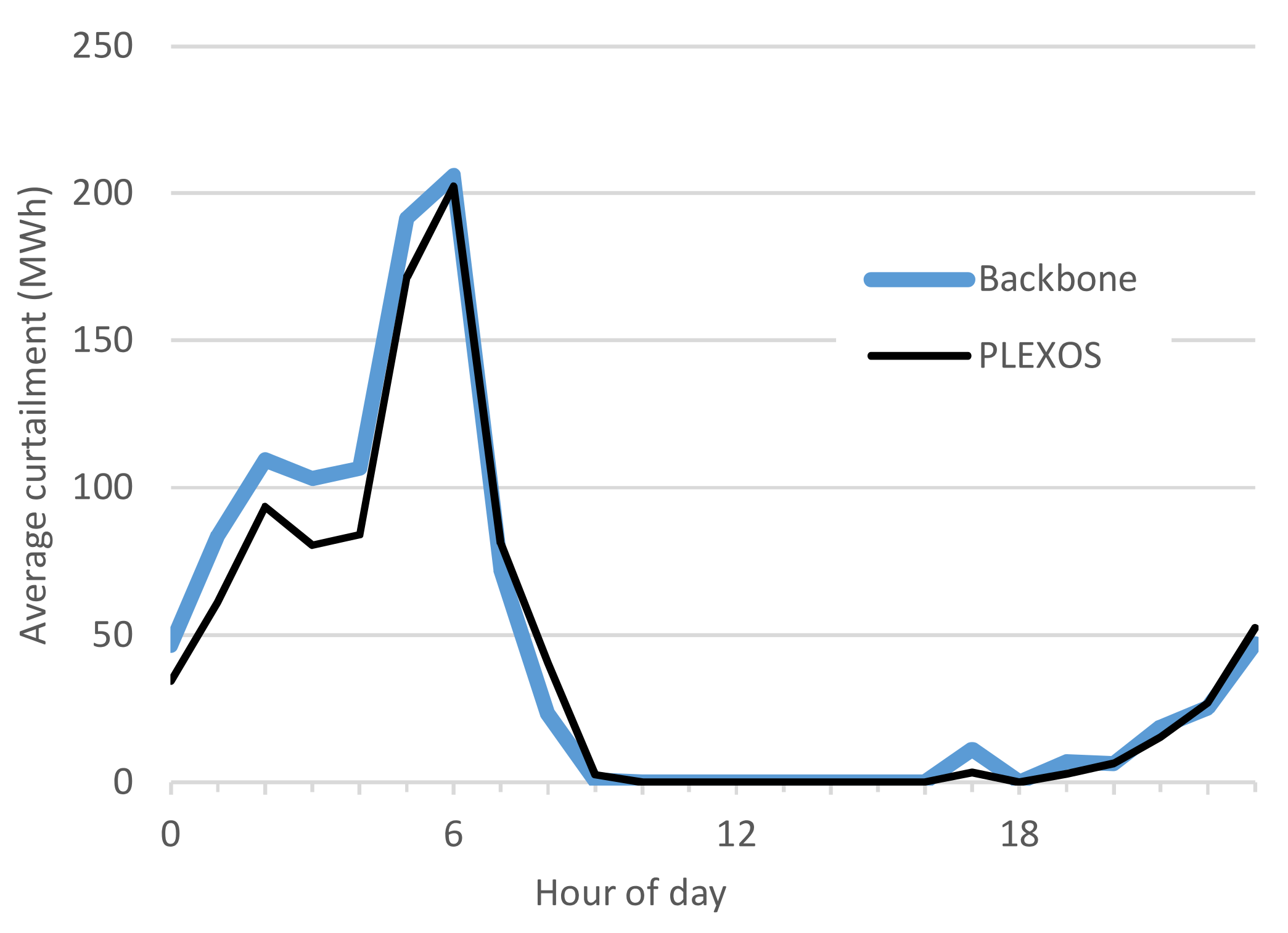
4.5. Comparison of Results
5. Discussion and Conclusions
Author Contributions
Funding
Conflicts of Interest
Nomenclature
| Indices and Sets | |
| Start-up types | |
| Start-up types which can only take place if the unit has not been offline for too long | |
| Emissions of fuel h | |
| Forecasts (, for realized and central forecasts) | |
| Forecast index; normally the same forecast as the current f except in the last interval of the stochastic horizon, in which case refers to the central forecast | |
| Forecast index; normally the same forecast as the current f except during the realized horizon, in which case refers to the realized forecast | |
| Forecast index; normally the same forecast as the current f except during the horizon when reserves have been locked / are to be locked, in which case refers to the realized forecast | |
| Main fuels of unit u | |
| Start-up fuels of unit u | |
| Incremental heat rate segments | |
| Indices for representing piecewise linear efficiency curves using -variables | |
| Nodes | |
| Nodes with a line to node | |
| Nodes that are in group | |
| Nodes where state needs to be the same in the first and last interval of a horizon | |
| Nodes where unit u has consumption capacity | |
| Nodes where unit u has production capacity | |
| Nodes with reserve demand | |
| Nodes with state variable | |
| Indices for state slacks (soft bounds) | |
| Reserve categories | |
| Downward reserves | |
| Upward reserves | |
| Samples | |
| Time intervals (, for the first and last time intervals) | |
| Units | |
| Units that have capacity in node n | |
| Conversion units taking input from node n and outputting to node | |
| Units that are in group | |
| Units using direct input to output conversion | |
| Units that have a possibility to trip | |
| Units using incremental heat rates for part-load efficiency representation | |
| Units that have consumption capacity in node n | |
| Units that have online variable | |
| Units that have production capacity in node n | |
| Units that have production capacity in node n and are in group | |
| Units that have ramping costs in node n | |
| Units that have start-up and shutdown trajectories | |
| Units using piecewise linear efficiency representation for part-load efficiencies (-variables) | |
| Forecast-interval combinations | |
| Lines | |
| Lines that are in group | |
| Node pairs with constrained state difference | |
| A bond between two inputs or outputs in a single unit (fixed ratio between the outputs/inputs) | |
| Nodes where state needs to be the same at the end of sample s and at the beginning of sample | |
| Node-unit combinations | |
| Indices for ramp tiers | |
| Time step index (an alternative for t, which is mainly used for intervals) | |
| Groups (for defining equations over a number of nodes, units, etc.), , , , | |
| Parameters | |
| Displacement to the previous interval, in time steps () | |
| Displacement to the shutdown decision if t is the last interval when unit u still needs to be offline, in time steps () | |
| Displacement to the start-up decision if unit u becomes online at interval t, in time steps () | |
| Displacement operator for aligning time frames (used with start-up and shutdown trajectories) | |
| Displacement to the interval when unit u became online if t is the last interval when the unit still needs to be online, in time steps () | |
| Line annuity factor based on number of periods n and rate per period r: , in (1/a) | |
| Unit annuity factor based on number of periods n and rate per period r: , in (1/a) | |
| Penalty of not meeting the balance equation, in CUR/MWh | |
| Soft upper or lower bound for the state of node n, in | |
| Reserve provision capability of line , in p.u. | |
| Reserve provision capability of unit u, in p.u. | |
| Multiplier of a unit investment variable when constraining the number of invested units for a group of units | |
| Maximum value for the sum of multiplied investment variables when constraining the number of invested units for a group of units | |
| Capacity margin, in MW | |
| Penalty of not meeting the capacity requirement, in CUR/MWh | |
| The ratio of one output or input to another output or input if the ratio of them is fixed | |
| Coefficient for energy diffusion between nodes, in MW/ | |
| Sign for the state slack direction, for upward boundaries and for downward boundaries | |
| Absolute lower limit of the state variable, in | |
| Incremental heat rate of segment | |
| Operating point related to segment , in p.u. | |
| Operating point of the -variable k, in p.u. | |
| Heat rate parameter representing no-load fuel consumption, calculated differently for direct conversion and incremental heat rate representation | |
| The slope of the linearized input/output curve | |
| The slope related to the -variable k | |
| Emission price or tax, in CUR/kg | |
| The last time step of sample s | |
| Fixed operational and maintenance costs, in CUR/MW(/a) | |
| Fuel and emission costs, in CUR/MWh | |
| Emission content in a fuel, in kg/MWh | |
| Fuel price, in CUR/MWh | |
| Inertia constant, in MJ/MVA | |
| Proportion of unit output that needs to be covered by reserves (preparing for a trip of the largest unit in node n), in p.u. | |
| External energy inflow/outflow, in MWh/h ( for consumption) | |
| Maximum instantaneous share of output | |
| Line investment costs, in CUR/MW | |
| Unit investment costs, in CUR/MW | |
| Maximum difference between the state of two nodes, in | |
| Maximum production/consumption capacity, in p.u. | |
| Maximum ramp down speed, in p.u./h | |
| Maximum ramp down speed of tier , in p.u./h | |
| Maximum ramp up speed, in p.u./h | |
| Maximum ramp up speed of tier , in p.u./h | |
| Maximum proportion of fuel h in normal operation | |
| Minimum production/consumption capacity, in p.u. | |
| Minimum production/consumption capacity, in p.u. | |
| Maximum value for the sum of multiplied online variables when constraining the number of online units for a group of units | |
| Multiplier of a unit online variable when constraining the number of online units for a group of units | |
| The probability or weight of interval | |
| Cost of ramping down, in CUR/MW | |
| Cost of ramping up, in CUR/MW | |
| Reserve demand, in MW | |
| Reserve demand increase caused by the output of unit u (typically preparing for variability and uncertainty), in p.u. | |
| Penalty of not meeting the reserve demand, in CUR/MWh | |
| Minimum rotational energy, in MJ | |
| Self-discharge rate of the node, in MW/ | |
| Cost of shutting down a unit, in CUR/unit | |
| Maximum production during the shutdown phase, in p.u. | |
| Minimum production during the shutdown phase, in p.u. | |
| The difference between the maximum and minimum ramping during the shutdown phase, in p.u./h | |
| Maximum ramping during the shutdown phase, in p.u./h | |
| Minimum ramping during the shutdown phase, in p.u./h | |
| Number of time steps needed for shutdown phase | |
| Capacity of a sub-unit, in MW. | |
| Consumption capacity of a sub-unit, in MW | |
| Production capacity of a sub-unit, in MW | |
| Capacity of a sub-unit, in MVA | |
| Unit conversion if state variable uses something else than MWh, in MWh/ | |
| The first time step of sample s | |
| Maximum time after shutdown when a start-up decision can be made, in time steps | |
| Minimum time after shutdown when a start-up decision can be made, in time steps | |
| Cost of starting up a unit, in CUR/unit | |
| Proportion of fuel h in start-up | |
| Start-up fuel use during the start-up phase, in MWh/unit | |
| Maximum production during the start-up phase, in p.u. | |
| Minimum production during the start-up phase, in p.u. | |
| The difference between the maximum and minimum ramping during the start-up phase, in p.u./h | |
| Maximum ramping during the start-up phase, in p.u./h | |
| Minimum ramping during the start-up phase, in p.u./h | |
| Number of time steps needed for start-up phase | |
| Increase in the upper limit of the state variable when investing in units, in /MW | |
| Penalty of exceeding the soft bounds of node states, in CUR//h | |
| Value of the node state, in CUR/ | |
| Number of sub-units | |
| Transfer capacity limit, in MW | |
| Transfer efficiency | |
| Absolute upper limit of the state variable, in | |
| Variable operational and maintenance costs, in CUR/MWh | |
| Length of interval , in h | |
| Variables | |
| Available capacity, in MW | |
| Dummy capacity to ensure capacity margin feasibility, in MW () | |
| Fixed operational and maintenance costs, in CUR(/a) | |
| Fuel and emission costs, in CUR | |
| Fuel use, in MWh/h () | |
| Conversion input () or output (), in MWh/h | |
| Production for each heat rate segment, in MWh/h | |
| Ramp from the previous interval to interval t, in MW/h | |
| Maximum production during the shutdown phase, in MWh/h | |
| Minimum production during the shutdown phase, in MWh/h | |
| Maximum production during the start-up phase, in MWh/h | |
| Minimum production during the start-up phase, in MWh/h | |
| Invested transfer capacity, in MW () | |
| Number of invested sub-units, in p.u. (, continuous or integer) | |
| Line investment costs, in CUR(/a) | |
| Objective function value, in CUR | |
| Number of sub-units online, in p.u. (, continuous or integer) | |
| Approximated online variable that takes into account start-up and shutdown trajectories, in p.u. | |
| Penalties, in CUR | |
| Ramping costs, in CUR | |
| Ramping down, in MW/h () | |
| Helper variable to relax ramp down constraint during the shutdown phase, in MW/h | |
| Helper variable to calculate ramp down variable and ramping costs during the shutdown phase, in MW/h | |
| Helper variable to relax ramp up constraint during the start-up phase, in MW/h | |
| Helper variable to calculate ramp up variable and ramping costs during the start-up phase, in MW/h | |
| Ramping up, in MW/h () | |
| Capacity reserved for providing reserves, in MW () | |
| Downward reserve provision impact to node n, summed over those units that have output capacity at node n and provide reserves to their input node, in MW | |
| Downward reserve provision impact to node n, summed over those units that have input capacity at node n and provide reserves to their output node, in MW | |
| Dummy to decrease reserve demand, in MW () | |
| Transfer capacity reserved for providing reserves, in MW () | |
| Upward reserve provision impact to node n, summed over those units that have output capacity at node n and provide reserves to their input node, in MW | |
| Upward reserve provision impact to node n, summed over those units that have input capacity at node n and provide reserves to their output node, in MW | |
| Number of sub-units shut down, in p.u. (, continuous or integer) | |
| Shutdown costs, in CUR | |
| Dummy consumption to ensure balance equation feasibility, in MWh/h () | |
| Dummy production to ensure balance equation feasibility, in MWh/h () | |
| Spill of energy from storage node, in MWh/h () | |
| Number of sub-units started up, in p.u. (, continuous or integer) | |
| Start-up costs, in CUR | |
| State variable (unit of measure depends on the application) | |
| Slack variable for state slack categories, in () | |
| Value of state change, in CUR | |
| Energy transfer from node n to node , in MWh/h | |
| Unit investment costs, in CUR(/a) | |
| Variable operational and maintenance costs, in CUR | |
| Ordered set of non-negative variables for piece-wise linear efficiency curve. At most two variables can be non-zero . If two variables are non-zero, they must be adjacent in the set. | |
| Abbreviations | |
| CC | Combined Cycle |
| CT | Combustion Turbine |
| CUR | Currency |
| GAMS | General Algebraic Modeling System |
| MIP | Mixed-integer Programming |
| PV | Photovoltaic |
| RTPV | Roof-top Photovoltaic |
| RTS-GMLC | Reliability Test System—Grid Modernization Lab Consortium |
| ST | Steam Turbine |
| VRE | Variable Renewable Energy |
References
- Loulou, R.; Remme, U.; Kanudia, A.; Lehtila, A.; Goldstein, G. Documentation for the TIMES Model Part I; Technical Report; IEA Energy Technology Systems Analysis Programme: Paris, France, 2005. [Google Scholar]
- Loulou, R.; Lehtila, A. Stochastic Programming and Tradeoff Analysis in TIMES; Technical Report; IEA Energy Technology Systems Analysis Programme: Paris, France, 2016. [Google Scholar]
- Panos, E.; Lehtilä, A. Dispatching and Unit Commitment Features in TIMES; Technical Report; IEA Energy Technology Systems Analysis Programme: Paris, France, 2016. [Google Scholar]
- Seljom, P.; Tomasgard, A. The impact of policy actions and future energy prices on the cost-optimal development of the energy system in Norway and Sweden. Energy Policy 2017, 106, 85–102. [Google Scholar] [CrossRef]
- Kannan, R.; Turton, H. A long-term electricity dispatch model with the TIMES framework. Environ. Model. Assess. 2013, 18, 325–343. [Google Scholar] [CrossRef]
- Blanco, H.; Nijs, W.; Ruf, J.; Faaij, A. Potential of Power-to-Methane in the EU energy transition to a low carbon system using cost optimization. Appl. Energy 2018, 232, 323–340. [Google Scholar] [CrossRef]
- Pina, A.; Silva, C.A.; Ferrão, P. High-resolution modeling framework for planning electricity systems with high penetration of renewables. Appl. Energy 2013, 112, 215–223. [Google Scholar] [CrossRef]
- Schrattenholzer, L. The Energy Supply Model MESSAGE; Technical Report; IIASA International Institute for Applied Systems Analysis: Laxenburg, Austria, 1981. [Google Scholar]
- Messner, S.; Golodnikov, A.; Gritsevskii, A. A stochastic version of the dynamic linear programming model MESSAGE III. Energy 1996, 21, 775–784. [Google Scholar] [CrossRef]
- Huppmann, D.; Gidden, M.; Fricko, O.; Kolp, P.; Orthofer, C.; Pimmer, M.; Kushin, N.; Vinca, A.; Mastrucci, A.; Riahi, K.; et al. The MESSAGEix Integrated Assessment Model and the ix modeling platform (ixmp): An open framework for integrated and cross-cutting analysis of energy, climate, the environment, and sustainable development. Environ. Modell. Softw. 2019, 112, 143–156. [Google Scholar] [CrossRef]
- Manzoor, D.; Aryanpur, V. Power sector development in Iran: A retrospective optimization approach. Energy 2017, 140, 330–339. [Google Scholar] [CrossRef]
- Howells, M.; Rogner, H.; Strachan, N.; Heaps, C.; Huntington, H.; Kypreos, S.; Hughes, A.; Silveira, S.; Decarolis, J.; Bazillian, M.; et al. OSeMOSYS: The Open Source Energy Modeling System: An introduction to its ethos, structure and development. Energy Policy 2011, 39, 5850–5870. [Google Scholar] [CrossRef]
- Welsch, M.; Deane, P.; Howells, M.; O Gallachóir, B.; Rogan, F.; Bazilian, M.; Rogner, H.H. Incorporating flexibility requirements into long-term energy system models—A case study on high levels of renewable electricity penetration in Ireland. Appl. Energy 2014, 135, 600–615. [Google Scholar] [CrossRef]
- E3MLab. PRIMES Model: Version 6, 2016–2017; Technical Report; E3MLab: Athens, Greece, 2016. [Google Scholar]
- Rosen, J. The Future Role of Renewable Energy Sources in European Electricity Supply: A Model-Based Analysis for the EU-15. Ph.D. Thesis, Universität Fridericiana zu Karlsruhe, Karlsruhe, Germany, 2008. [Google Scholar] [CrossRef]
- DNV GL; Imperial College; NERA Economic Consulting. Integration of Renewable Energy in Europe; Technical Report; DNV GL: Bonn, Germany, 2014. [Google Scholar]
- Collins, S.; Deane, J.P.; Ó Gallachóir, B. Adding value to EU energy policy analysis using a multi-model approach with an EU-28 electricity dispatch model. Energy 2017, 130, 433–447. [Google Scholar] [CrossRef]
- Powell, W.B.; George, A.; Simão, H.; Scott, W.; Lamont, A.; Stewart, J. SMART: A Stochastic Multiscale Model for the Analysis of Energy Resources, Technology, and Policy. INFORMS J. Comput. 2012, 24, 665–682. [Google Scholar] [CrossRef]
- Lamont, A. User’s Guide to the META-Net Economic Modeling System—Version 1.2; Technical Report; Lawrence Livermore National Laboratory: Livermore, CA, USA, 1994. [Google Scholar]
- Pfenninger, S.; Keirstead, J. Renewables, nuclear, or fossil fuels? Scenarios for Great Britain’s power system considering costs, emissions and energy security. Appl. Energy 2015, 152, 83–93. [Google Scholar] [CrossRef]
- Welder, L.; Ryberg, D.S.; Kotzur, L.; Grube, T.; Robinius, M.; Stolten, D. Spatio-temporal optimization of a future energy system for power-to-hydrogen applications in Germany. Energy 2018, 158, 1130–1149. [Google Scholar] [CrossRef]
- Ravn, H.F.; Hindsberger, M.; Petersen, M.; Schmidt, R.; Bøg, R.; Grohnheit, P.E.; Larsen, H.V.; Munksgaard, J.; Ramskov, J.; Esop, M.R.; et al. Balmorel: A Model for Analyses of the Electricity and CHP Markets in the Baltic Sea Region; Technical Report; Elkraft System: Ballerup, Denmark, 2001. [Google Scholar]
- Wiese, F.; Bramstoft, R.; Koduvere, H.; Pizarro Alonso, A.; Balyk, O.; Kirkerud, J.G.; Tveten, Å.G.; Bolkesjø, T.F.; Münster, M.; Ravn, H. Balmorel open source energy system model. Energy Strategy Rev. 2018, 20, 26–34. [Google Scholar] [CrossRef]
- Scholz, Y. Renewable Energy Based Electricity Supply at Low Costs: Development of the REMix Model and Application for Europe. Ph.D. Thesis, Unversity of Stuttgart, Stuttgart, Germany, 2012. [Google Scholar] [CrossRef]
- Gerhardt, N.; Sandau, F.; Scholz, A.; Hahn, H.; Schumacher, P.; Sager, C.; Bergk, F.; Kämper, C.; Knörr, W.; Kräck, J.; et al. Interaktion EE-Strom, Wärme und Verkehr: Endbericht; Technical Report; Fraunhofer IWES, Fraunhofer IBP, IFEU, and Stiftung Umweltenergierecht: Kassel, Germany, 2015. [Google Scholar]
- Short, W.; Sullivan, P.; Mai, T.; Mowers, M.; Uriarte, C.; Blair, N.; Heimiller, D.; Martinez, A. Regional Energy Deployment System (ReEDS); Technical Report; National Renewable Energy Laboratory (NREL): Golden, CO, USA, 2011. [Google Scholar]
- Pfenninger, S.; DeCarolis, J.; Hirth, L.; Quoilin, S.; Staffell, I. The importance of open data and software: Is energy research lagging behind? Energy Policy 2017, 101, 211–215. [Google Scholar] [CrossRef]
- Kiviluoma, J.; Rinne, E.; Rasku, T.; Helistö, N.; Kirchem, D.; Li, R.; O’Dwyer, C. Backbone Modelling Tool, Version 1.1. 2019. Available online: https://gitlab.vtt.fi/backbone/backbone/tags/v1.1 (accessed on 16 August 2019).
- Bakirtzis, E.A.; Biskas, P.N.; Labridis, D.P.; Bakirtzis, A.G. Multiple Time Resolution Unit Commitment for Short-Term Operations Scheduling Under High Renewable Penetration. IEEE Trans. Power Syst. 2014, 29, 149–159. [Google Scholar] [CrossRef]
- De Farias, I.R.; Zhao, M.; Zhao, H. A special ordered set approach for optimizing a discontinuous separable piecewise linear function. Oper. Res. Lett. 2008, 36, 234–238. [Google Scholar] [CrossRef]
- Barrows, C.; Bloom, A.; Ehlen, A.; Ikäheimo, J.; Jorgenson, J.; Krishnamurthy, D.; Lau, J.; McBennett, B.; O’Connell, M.; Preston, E.; et al. The IEEE Reliability Test System: A Proposed 2019 Update. IEEE Trans. Power Syst. 2019, in press. [Google Scholar] [CrossRef]
- Grigg, C.; Wong, P.; Albrecht, P.; Allan, R.; Bhavaraju, M.; Billinton, R.; Chen, Q.; Fong, C.; Haddad, S.; Kuruganty, S.; et al. The IEEE Reliability Test System-1996. A report prepared by the Reliability Test System Task Force of the Application of Probability Methods Subcommittee. IEEE Trans. Power Syst. 1999, 14, 1010–1020. [Google Scholar] [CrossRef]
- Github—GridMod/RTS-GMLC. Available online: https://github.com/GridMod/RTS-GMLC (accessed on 10 March 2019).
- Software Solutions. Available online: https://energyexemplar.com/ (accessed on 10 March 2019).
- Stoll, B.; Brinkman, G.; Townsend, A.; Bloom, A. Analysis of Modeling Assumptions Used in Production Cost Models for Renewable Integration Studies; Technical Report; National Renewable Energy Laboratory (NREL): Golden, CO, USA, 2016. [Google Scholar]
- Rasku, T.; Kiviluoma, J. A comparison of widespread flexible residential electric heating and energy efficiency in a future nordic power system. Energies 2019, 12, 5. [Google Scholar] [CrossRef]
- Tejada-Arango, D.A.; Morales-España, G.; Wogrin, S.; Centeno, E. Power-based generation expansion planning for flexibility requirements. arXiv 2019, arXiv:1902.07779. [Google Scholar]


| Plant Type | PLEXOS | Backbone |
|---|---|---|
| Coal | 570.3 | 578.6 |
| Gas | 445.5 | 438.2 |
| Solar | 255.3 | 254.3 |
| Hydro | 219.1 | 219.1 |
| Wind | 169.3 | 168.9 |
| Nuclear | 134.2 | 134.2 |
| Oil | 0.4 | 0.7 |
| Cost Type | PLEXOS | Backbone |
|---|---|---|
| Fuel cost | 26.49 | 26.49 |
| Start-up and shutdown cost | 0.52 | 0.48 |
| Total | 27.01 | 26.97 |
© 2019 by the authors. Licensee MDPI, Basel, Switzerland. This article is an open access article distributed under the terms and conditions of the Creative Commons Attribution (CC BY) license (http://creativecommons.org/licenses/by/4.0/).
Share and Cite
Helistö, N.; Kiviluoma, J.; Ikäheimo, J.; Rasku, T.; Rinne, E.; O’Dwyer, C.; Li, R.; Flynn, D. Backbone—An Adaptable Energy Systems Modelling Framework. Energies 2019, 12, 3388. https://doi.org/10.3390/en12173388
Helistö N, Kiviluoma J, Ikäheimo J, Rasku T, Rinne E, O’Dwyer C, Li R, Flynn D. Backbone—An Adaptable Energy Systems Modelling Framework. Energies. 2019; 12(17):3388. https://doi.org/10.3390/en12173388
Chicago/Turabian StyleHelistö, Niina, Juha Kiviluoma, Jussi Ikäheimo, Topi Rasku, Erkka Rinne, Ciara O’Dwyer, Ran Li, and Damian Flynn. 2019. "Backbone—An Adaptable Energy Systems Modelling Framework" Energies 12, no. 17: 3388. https://doi.org/10.3390/en12173388
APA StyleHelistö, N., Kiviluoma, J., Ikäheimo, J., Rasku, T., Rinne, E., O’Dwyer, C., Li, R., & Flynn, D. (2019). Backbone—An Adaptable Energy Systems Modelling Framework. Energies, 12(17), 3388. https://doi.org/10.3390/en12173388