Optimal Dispatching of Offshore Microgrid Considering Probability Prediction of Tidal Current Speed

Abstract

Oceans contain rich tidal current energy, which can provide sufficient power for offshore microgrids. However, the uncertainty of tidal flow may endanger the operational reliability of an offshore microgrid. In this paper, a probabilistic prediction model of tidal current is established based on support vector quantile regression to reduce the influence of uncertainty. Firstly, the penalty factors and kernel parameters of the proposed prediction model was optimized by the dragonfly algorithm to predict the tidal speed of any time of a day in different quantiles. Secondly, combining the above result with the kernel density to predict the probability density function of the tidal current speed, which is to improve the accuracy of prediction in the absence of information. Thirdly, an optimal generation dispatching strategy with tidal current generators is proposed to minimize the fuel consumption of offshore microgrids. Finally, a case study based on the offshore oil and gas platform in Bohai shows that the mean absolute percent error of the proposed model is 2.8142%, which is better than support vector quantile regression model and support vector regression model optimized by the genetic algorithm.

1. Introduction

An offshore microgrid is an effective way to provide energy for offshore platforms, which can deal with the limited fossil resources issues through using renewable energy generators and energy storage devices [1,2]. At present, offshore renewable energy mainly includes solar energy, wind energy, ocean temperature difference energy, tidal current energy and so on, among which the tidal current power has recently received widely concerned due to its vast reserves and high energy density [3,4,5,6]. However, the tide current has strong randomness owing to the wave, sea breeze, temperature, etc. Therefore, it is essential to establish the prediction model of tidal current speed to make efficient use of the tidal current energy in that an accurate prediction can achieve sophisticated strategies to guarantee a stable energy source for offshore microgrids, thereby saving economic cost [7].

The harmonic analysis method (HAM), which is to decompose complex tidal flow curves into several harmonic terms, calculate harmonic coefficient changes and the astronomic effect, has been widely used in tidal current prediction [8,9]. The height of the tidal current is considered as a set of harmonic components in the HAM. The amplitude and phase of each harmonic component can be inferred from the historical data of the tidal by the least squares method [10]. Then, the tidal current speed can be calculated based on the tidal current height [11]. However, the method suffers from two critical drawbacks. (a) They require large historical datasets (several years), and (b) they have inefficient performances for predicting sudden and aperiodic patterns resulting from weather-based factors. When the observed tidal current data time interval less than or equal to one hour, there will exist non-harmonic components in it because of supra-tidal fluctuations. As a result, it cannot be modeled by conventional harmonic analysis—based on the prediction models. In recent years, to overcome these barriers and consider the nature of tidal current and the weather-based irregularities, machine learning-based prediction models have been proposed. Primarily, artificial neural network (ANN) and support vector machine are widely used, which can reduce the training period effectively [12,13,14]. Reference [12] proposed a hybrid model of an ANN and Fourier series model based on the least squares method (FLSM) to predict the speed and direction of the tidal current. Reference [13] proposed an accurate hybrid method based on support vector regression (SVR) and autoregressive integrated moving average (ARIMA) to predict the tidal current speed and direction. In the proposed hybrid model, the ARIMA model captures the linear component of the tidal current, and the SVR models the remaining components. A univariate prediction method based on wavelet transform and SVR was proposed in [14], where tidal current data was decomposed into some subharmonic components. The Wakeby distribution was also used to capture the probability characteristics of the tidal current speed. Since the timing of the tidal flow velocity is not taken into consideration, and the error with the actual data in a short time, this model cannot directly be used to predict the tidal velocity time series [15,16,17]. Therefore, the k-means clustering technique and non-parametric kernel density estimation method were used to model the random components of the tidal current speed [18,19,20]. However, the deterministic techniques used in the above literature do not take into account the timing of the tidal speed, and the single-point prediction may cause relatively large errors. For example, the Weibull distribution [21] and the Wakeby distribution do not take into account in the time-series data. Moreover, the single-point prediction using ANN and support vector machine (SVM) cannot fully reflect the uncertainty of the tidal current power generation. Furthermore, the tidal data is highly seasonal, containing carious cycles. In other words, tidal information naturally includes a specific amount of uncertainty, which is produced by its volatile and random characteristics. Therefore, the probabilistic-prediction was adopted in this paper to improve the accuracy of the model because it can better describe the possible fluctuation of future tidal current power generation better. It is conducive to the timely adjustment of the offshore engineering plan and the optimal scheduling of the offshore microgrid.

Economic dispatch (ED) is to determine the optimal output power of multiple generator sets and meet the system load demand problem at the lowest cost [22]. In the reference [23,24], multi-objective optimization scheduling models were established under the environmental and economic factors. Reference [25] proposed multi-objective optimization problems for solving the power system using the artificial swarm algorithm. In reference [26], the three-objective optimal dispatching model was transformed into a single-objective optimal dispatching model, which was solved by the interior point method to obtain the optimal solution. The dynamic optimization dispatching model is more suitable for the offshore microgrid with the tidal current because the power of tidal current generators will change with the tidal current velocity. Therefore, it is necessary to predict the output of tidal current generators for each time period.

In this paper, we proposed a time-sequential probabilistic prediction model based on support vector quantile regression (SVQR) and kernel density estimation. By using the dragonfly algorithm, the parameters of the model are optimized, which not only improved the prediction accuracy but also obtained the fluctuation range of future tidal current speed. Besides, the optimization model of an offshore microgrid with tidal current power generation was established by taking into account indicators such as economic cost and environmental benefits. In order to improve the solving speed and obtain the globally optimal solution, the dragonfly algorithm was applied. The proposed method has proven to be efficient and correct when applied to a case of an offshore oilfield microgrid using tidal current energy.

This paper is organized as follows: The prediction model and the basic theory are introduced in Section 2, followed by an economic dispatching model of an offshore microgrid based on tidal velocity prediction in Section 3. Section 4 presents the results of the case analysis. Concluding remarks are given in Section 5.

2. Prediction Models and Basic Theories

The structural diagram of the offshore microgrid is shown in Figure 1. The system mainly includes renewable energy power generation units, a gas turbine unit, an energy storage unit and an emergency power unit. Renewable energy refers to the tidal current in this paper.

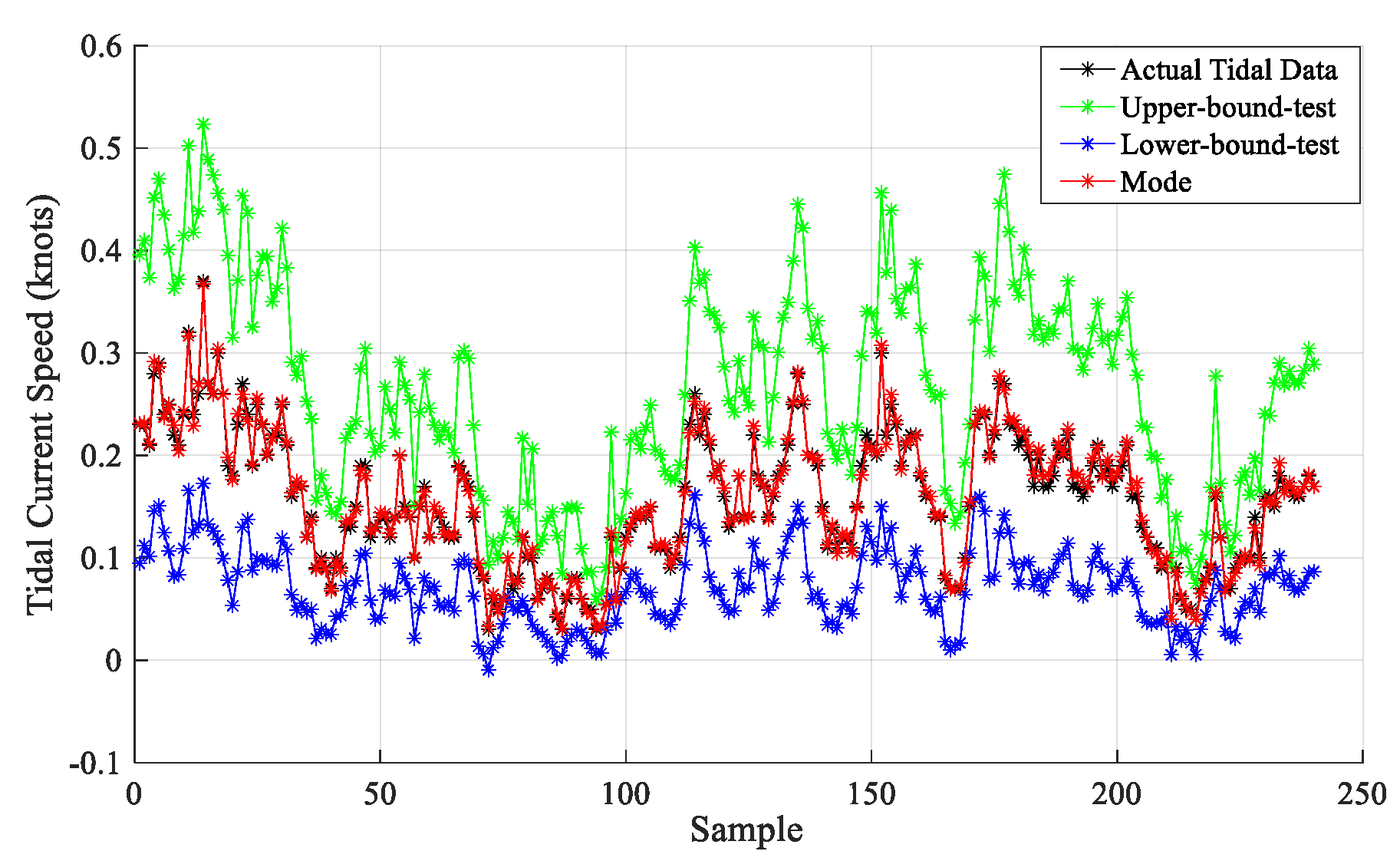
2.1. Support Vector Quantile Regression Based Probablity Prediction Model for Tidal Current Speed

Using the SVM will result in the deviation of single point prediction of tidal current speed due to the uncertainty of the tidal current energy output and the inherent defects of existing prediction models. However, compared with the single-point value prediction, the regression analysis under different quantiles can describe the influence of the distribution characteristics of input variables more completely. The quantile regression provides powerful theoretical support for probabilistic predictions. Therefore, useful information can be obtained for more accurate scientific decisions [27,28]. The quantile regression is based on the conditional quantile of the response variable y to predict the explanatory variable x, which can reflect the information that the explanatory variable x affects the position, distribution and shape of the response variable y in different ranges more closely. It has the following advantages: (1) Robustness, the quantile does not make any assumption for the distribution of random errors in the model; (2) resistance to outliers data, the quantile regression can be used from 0 to 1 and (3) parameters estimated by quantile have asymptotic optimality under large samples.

The main parameters are explained in

Table 1. Parameter interpretation.

x, xi	Explanatory Variables
y, yi	Response variables
Qyi	Linear regression estimate
β(τ)	Regression coefficient vector
τ	Quantile
σ	Free parameter of the kernel parameter
C	Penalty parameter

:

Assume that the sample set of the tidal current speed and its related historical data can be represented as $G={\left\{(x_i,y_i)\right\}}_{i=1}^n$, where x_i is the input sample vector containing historical tidal current rate and is considered as explanatory variables, and y_i is the corresponding output sample of the tidal current speed and is considered as the response variables. Then the linear quantile regression model of tidal current speed is:

$$Q_{y_i}(\tau |x)={\beta }_0(\tau )+{\beta }_1(\tau )x_1+{\beta }_2(\tau )x_2+\cdots +{\beta }_k(\tau )x_k\equiv x_i^{\prime }\beta (\tau ).$$

(1)

Here, Q_yi(τ|x) is the τ-th conditional quantile of the response variables y under the explanatory variables x = [x₁,x₂,…,x_i]^T. When τ is continuously taken in the interval (0,1), the conditional distribution of the response variable can be obtained. β(τ) is the regression coefficient vector, it changes as the quantile changes. The estimation of β(τ) in the above equation can be formulated as follows:

$$\underset{\beta }{\min }{\displaystyle \sum _{i=1}^n{\beta }_{\tau }(y_i-x_i^{\prime }\beta )}=\underset{\beta }{\min }{\displaystyle \sum _{i\left|y_i\ge x_i^{\prime }\beta \right|}\tau }\left|y_i-x_i^{\prime }\beta \right|+{\displaystyle \sum _{i\left|y_i<x_i^{\prime }\beta \right|}(1-\tau )}\left|y_i-x_i^{\prime }\beta \right|.$$

(2)

The prediction precision of tidal current speed is affected by a variety of complex factors in a linear or non-linear manner. However, the quantile regression mentioned above is based on linear regression, which is difficult to solve complex nonlinear functions. Therefore, a semiparametric method is adopted to optimize the combination of the support vector machine regression (SVR) [29] and the quantile regression (QR) to obtain the support vector quantile regression (SVQR) model of tidal current speed. Based on the SVR model, the penalty parameter part is replaced by quantile regression. As a result, the SVQR model is expressed as follows:

$$\underset{w_{\tau },b_{\tau }}{\min }\frac{1}{2}{\Vert w_{\tau }\Vert }^2+C{\displaystyle \sum _{i=1}^I{\rho }_{\tau }(y_i-b_{\tau }-w_{\tau }^T\varphi (x_i))}.$$

(3)

Here, C is a penalty parameter, w_τ and b_τ represent the weight and deviation of the τ-th conditional quantile respectively and φ(x) is a nonlinear mapping function.

According to the theory of structural risk minimization, and satisfying the solution to the optimization problem, the slack variables $\vartheta$ and ${\vartheta }^{\ast }$ are introduced. The SVM regression model can be expressed as:

$$\begin{array}{l}\underset{w_{\tau },b_{\tau },{\vartheta }_{i,}{\vartheta }_i^{*}}{\min }\frac{1}{2}{\Vert {\omega }_{\tau }\Vert }^2+C{\displaystyle \sum _{i=1}^I(}\tau {\vartheta }_i+(1-\tau ){\vartheta }_i^{*})\\ \mathrm{S}.\mathrm{T}.\{\begin{array}{l}{y}_i-{\omega }_{\tau }^T\phi (x_i)-b_{\tau }\le \epsilon +{\vartheta }_i,i=1,2,\cdots ,N\\ {\omega }_{\tau }^T\phi (x_i)+b_{\tau }-y_i\le \epsilon +{\vartheta }_i{}^{*},i=1,2,\cdots ,N\\ {\vartheta }_i\ge 0;{\vartheta }_i{}^{*}\ge 0\end{array}\end{array}$$

(4)

To solve the convex quadratic optimization problem of the above formula, the objective function and Lagrange function constraints are combined to convert the nonlinear programming problem into a dual problem.

Lagrange function is as follows:

$$\begin{array}{l}{L}_{\tau }(w_{\tau },b_{\tau },{\vartheta }_i,{\vartheta }_i^{*};{\alpha }_{\tau i},{\alpha }_{\tau i}^{*},{\xi }_{\tau i},{\xi }_{\tau i}^{*})=\frac{1}{2}{\Vert w_{\tau }\Vert }^2-{\displaystyle \sum _{i=1}^I{\alpha }_{\tau i}({\vartheta }_i-y_i+w_{\tau }\phi (x_i)+b_i)}-\\ {\displaystyle \sum _{i=1}^I{\alpha }_{\tau i}^{*}({\vartheta }_i+y_i-w_{\tau }\phi (x_i)-b_i)}+C{\displaystyle \sum _{i=1}^I(\tau {\vartheta }_i+(1-\tau ){\vartheta }_i^{*})}-{\displaystyle \sum _{i=1}^I({\xi }_{\tau i}{\vartheta }_i+{\xi }_{\tau i}^{*}{\vartheta }_i^{*})}\end{array}$$

(5)

Here, Lagrange multipliers at different quantiles are ${\alpha }_{\tau i},{\alpha }_{\tau i}^{*},{\xi }_{\tau i},{\xi }_{\tau i}^{*}\ge 0 (i=1,2,\cdots I)$, then the first partial derivative of $w_{\tau },b_{\tau },{\vartheta }_i,{\vartheta }_i^{*}$ in function L_τ are obtained by formula (6).

$$S.T.\{\begin{array}{l}\frac{\partial L_{\tau }}{\partial w_{\tau }}=0\Rightarrow w_{\tau }={\displaystyle \sum _{i=1}^I({\alpha }_{\tau i}-{\alpha }_{\tau i}^{*})}\phi (x_i),\\ \frac{\partial L_{\tau }}{\partial b_{\tau }}=0\Rightarrow {\displaystyle \sum _{i=1}^I({\alpha }_{\tau i}-{\alpha }_{\tau i}^{*})}=0,\\ \frac{\partial L_{\tau }}{\partial {\vartheta }_i}=0\Rightarrow \tau C-{\alpha }_{\tau i}-{\xi }_{\tau i}=0,\\ \frac{\partial L_{\tau }}{\partial {\vartheta }_i^{*}}=0\Rightarrow (1-\tau )C-{\alpha }_{{}_{\tau i}}^{*}-{\xi }_{{}_{\tau i}}^{*}=0\end{array}.$$

(6)

The dual optimization problem of the above formula can be obtained by the dual principles, as follows:

$$\begin{array}{l}\underset{{\alpha }_{\tau i},{\alpha }_{{}_{\tau i}}^{*}}{\max }\left[-\frac{1}{2}{\displaystyle \sum _{i=1}^n{\displaystyle \sum _{j=1}^n({\alpha }_{\tau i}-{\alpha }_{{}_{\tau i}}^{*})({\alpha }_{\tau j}-{\alpha }_{{}_{\tau j}}^{*})K(x_i,x_j)+}}{\displaystyle \sum _{i=1}^I{\alpha }_{\tau i}(y_i-\epsilon )-{\displaystyle \sum _{i=1}^I{\alpha }_{{}_{\tau i}}^{*}(y_i-\epsilon )}}\right]\\ \mathrm{S}.\mathrm{T}.\{\begin{array}{c}{\displaystyle \sum _{i=1}^I({\alpha }_{\tau i}-{\alpha }_{{}_{\tau i}}^{*})=0,}\\ \begin{array}{l}0\le {\alpha }_{\tau i}\le \tau C,\\ 0\le {\alpha }_{{}_{\tau i}}^{*}\le (1-\tau )C\end{array}\end{array}\end{array}$$

(7)

Here, $K(x_i,x_j)=\exp \left(-{\Vert x_i-x_j\Vert }^2/2{\sigma }^2\right)$ is the kernel function, which represents the inner product of high-dimensional space, $a_{\tau i}$ and $a_{\tau i}^{*}$ are Lagrange factors.

Using the kernel function make it easier to calculate nonlinear predictions because it maps the nonlinear sample data into the higher-dimensional Hilbert space, making them linearly separable. Therefore, the problem of solving a decision function is transformed into how to select an appropriate and effective kernel function. The radial kernel function was applied in this paper.

The dual problem above is solved by introducing a kernel function as follows:

$$\{\begin{array}{l}{w}_{\tau }={\displaystyle \sum _{i=1}^I({\alpha }_{\tau i}-{\alpha }_{{}_{\tau i}}^{*})\phi (x_i)}\\ b_{\tau }=average\left|\epsilon \mathrm{sgn}({\alpha }_{\tau i}-{\alpha }_{{}_{\tau i}}^{*})+y_i-{\displaystyle \sum _{i=1}^I({\alpha }_{\tau i}-{\alpha }_{{}_{\tau i}}^{*})K(x_i,x)}\right|\end{array}.$$

(8)

Therefore, the formula of the SVQR model is as follows:

$$Q_{y\tau }(\tau |x)=w_{{}_{\tau }}^T\phi (x_i)+b_{\tau }.$$

(9)

Here, η = (C, σ) is the hyper-parameter set of SVQR model needed to be optimized, C is the penalty parameter and σ is the free parameter of the kernel parameter.

Based on the above research, first obtain the different quantiles of the tidal current speed prediction results Q_yτ(τ|x), and then use the quantile at different quantiles as the input value of kernel density estimation to predict the probability density function. Kernel density estimation is a non-parametric estimation method with high prediction accuracy that can be used for analysis of any distribution sample. Assuming v₁, v₂ … v_n are n sample values of tidal current speed, the kernel density estimation is defined as:

$$f(x)=\frac{1}{nh}{\displaystyle \sum _{i=1}^{n}K(\frac{v-v_i}{h})}.$$

(10)

Here, h is bandwidth and K is the kernel density function.

The accuracy of f(x) depends on the kernel function and the bandwidth coefficient. This paper adopted the Gaussian kernel function below as follows:

$$K(u)=\frac{1}{\sqrt{2\pi }}{e}^{-u^2/2}.$$

(11)

When the bandwidth is fixed, the choice of it is essential because the effect of different kernel functions on probability density function is equivalent. The bandwidth is employed as:

$$h=1.06\sigma n^{-\frac{1}{5}}.$$

(12)

Here, σ is the standard deviation of the random variable x.

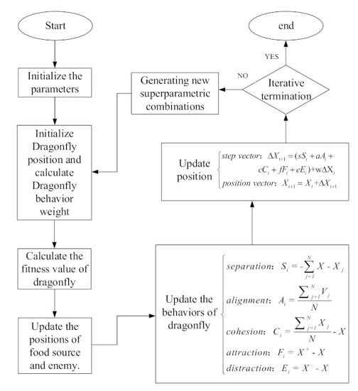
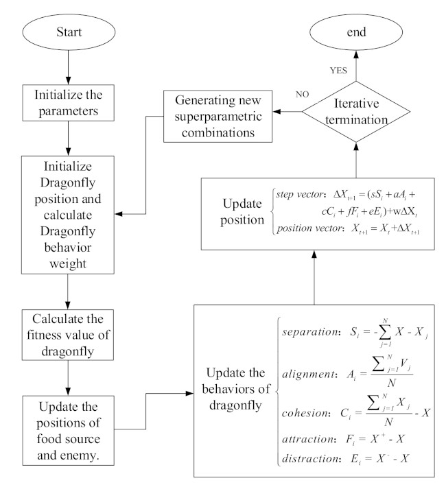
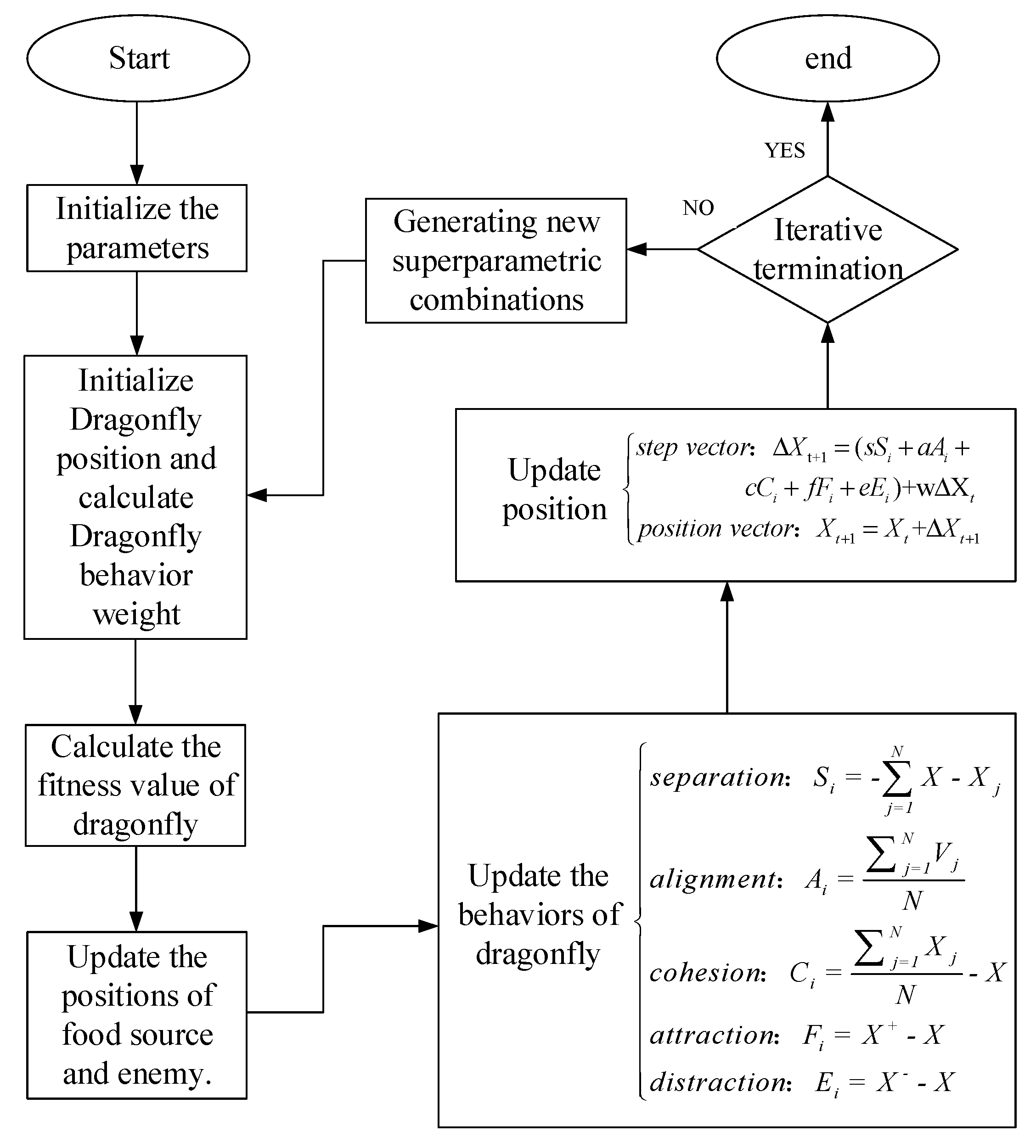
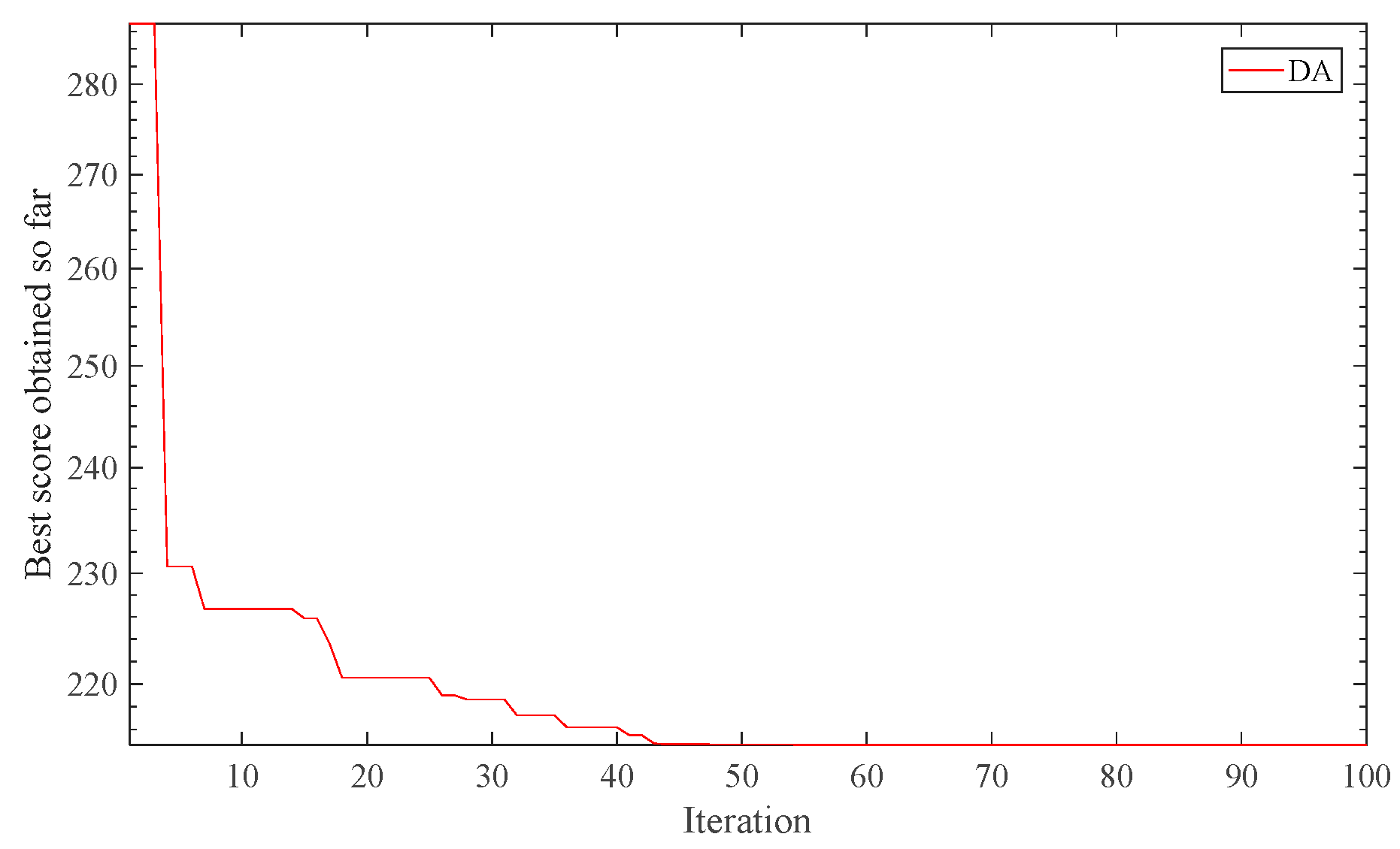
2.2. Probablistic Prediction Model of Tidal Current Speed Nased on Dragonfly Algorithm

The dragonfly algorithm (DA) is a novel swarm intelligence optimization algorithm that put forward by Seyedali Mirjalili in 2015 [30]. Two distinct group behaviors of predation (static behavior) and migration (dynamic group behavior) of the dragonfly guarantee the stability, fast speed and global optimization abilities.

In the SVQR model, C is a penalty parameter. The larger C is, the less error of the model is allowed, and the worse the generalization ability is. σ is also the kernel parameter, which is the value of the kernel parameter that determines the distribution of the nonlinear input vector that mapped into a high-dimensional feature space. Therefore, the selection of parameter C and σ directly affects the regression prediction performance of the SVQR model. Since the dragonfly algorithm has the advantage of the fast convergence and global optimization, this paper proposed a DA-SVQR regression prediction model, which improved the accuracy of the prediction model effectively.

The parameter optimization steps of the DA-SVQR algorithm are as follows:

Step 1: Initialize the parameters. The main parameters of the dragonfly algorithm include the number of dragonfly individuals, the dimension of the problem and the maximum iteration number. The main parameters of SVQR model include penalty parameter C, and upper and lower limits of kernel parameter.

Step 2: Set up the training number sets, training number labels, test sets and test set labels.

Step 3: Initialize dragonfly position. Initialization generates Dragonfly position X₀ and initialization step vector ΔX_t. The hyper-parametric η in the SVQR model that needs to be optimized is taken as the location of the dragonfly solution X_t.

Step 4: Calculate individual weight values. Randomly initialize the neighboring radius (r) and the inertia weight (w), randomly initialize the weights of five behaviors of a dragonfly individual, i.e., separation weight (s), alignment weight (a), cohesion weight (c), weight of attraction to food (f) and weight of distraction from an enemy (e)

Step 5: Calculate the fitness value of the dragonfly. The classification accuracy of the model is taken as the current fitness value of the individual dragonfly. Whenever a position update is performed, the current maximum fitness value is calculated and recorded. If the fitness value of the current dragonfly is higher than the saved fitness value, the former is taken as the optimal one, then preserves the current optimal value as a corresponding hyper-parametric η, otherwise it retains the original fitness value and the corresponding hyper-parametric η.

Step 6: Update the resource of food and the enemy position. The Euclidean distance formula is used to calculate the food source (X⁺) and enemy position (X⁻).

Step 7: Update the behaviors of the dragonfly. Update the five behaviors of dragonfly individual: Separation (S), alignment (A), cohesion (C), attraction to food (F) and distraction from enemies (E).

Step 8: Update position. If there is at least one neighboring dragonfly, then update the step and position vectors. If there is no neighboring dragonfly, and then update the position vector.

Step 9: Algorithm iteration termination judgment. When the maximum iteration count appears, the current optimal position vector will be saved and regarded as the optimal combination. Otherwise, the number of iterations adds up to 1, then go to step 4.

The flow chart of SVQR is shown in Figure 2.

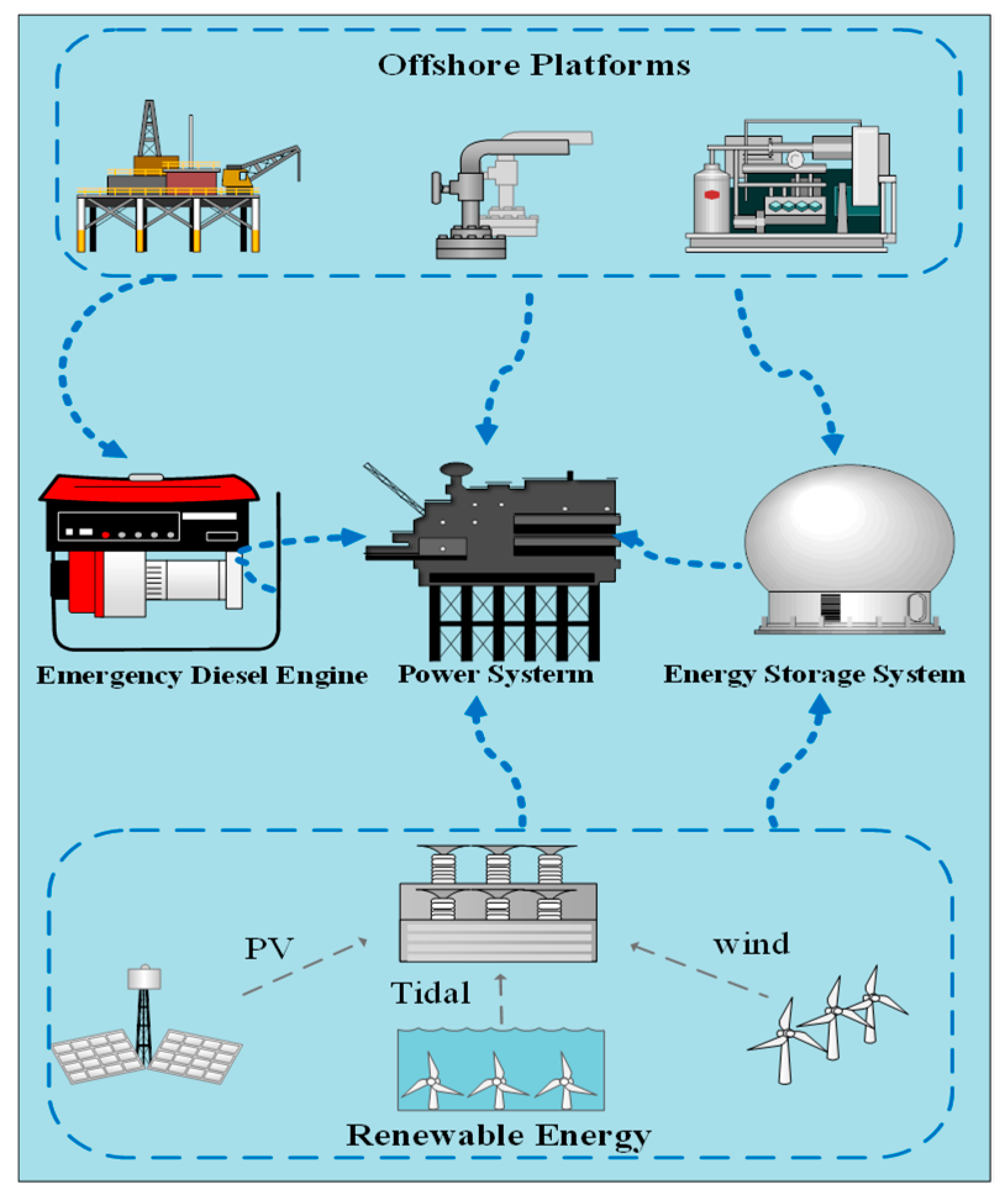
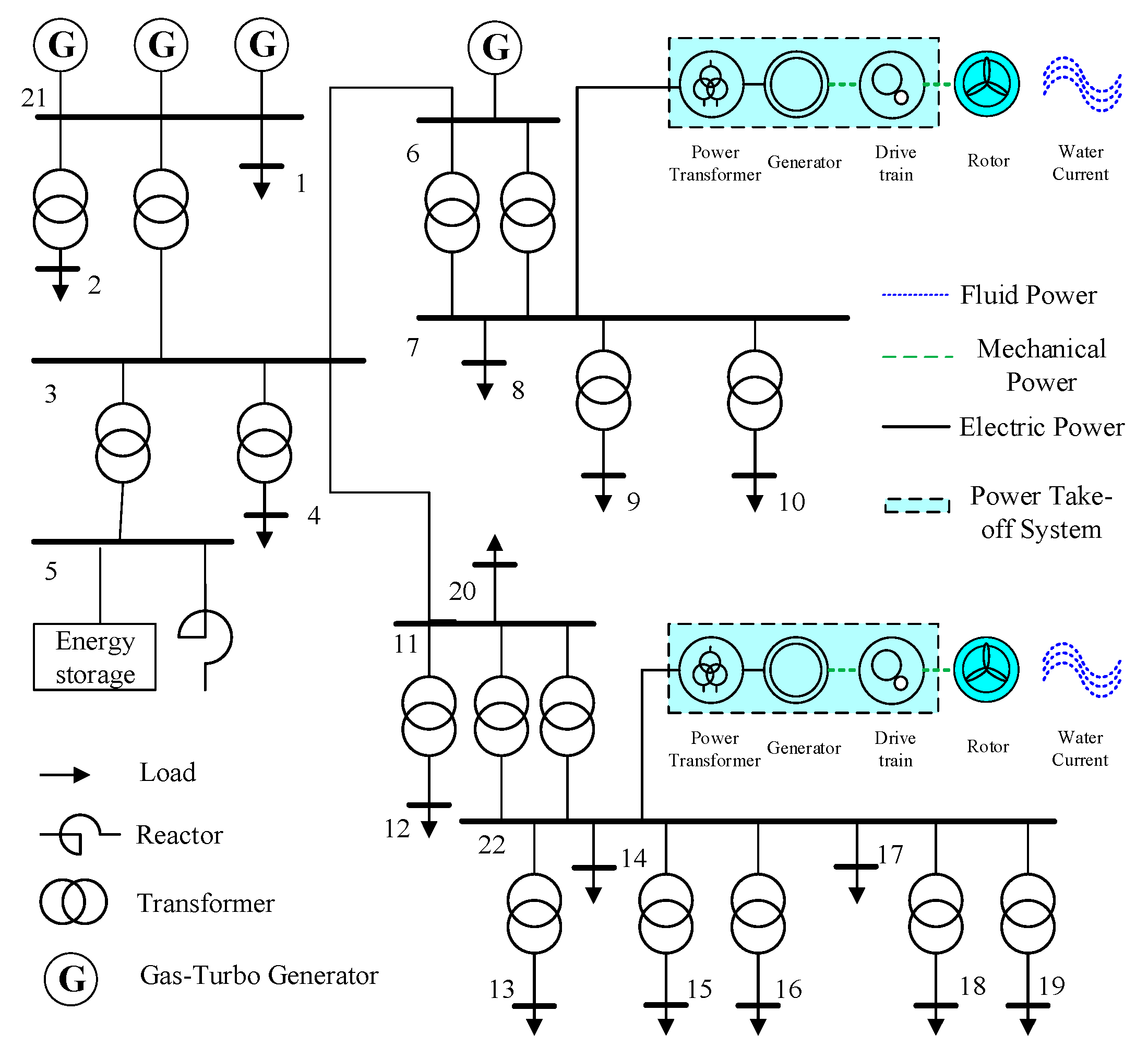
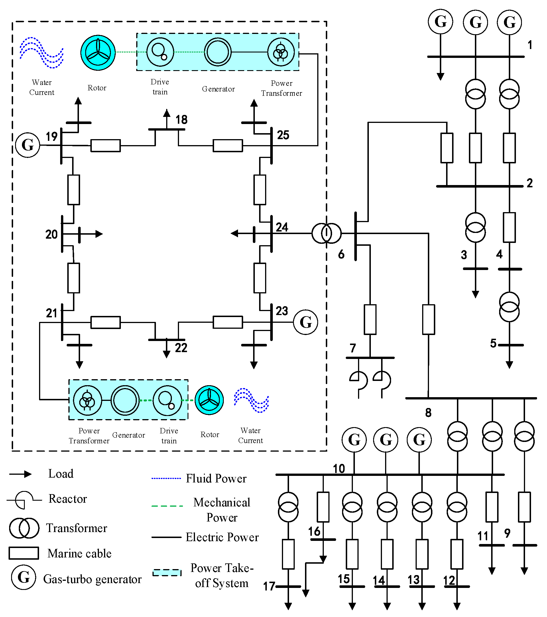
3. Optimal Dispatching of the Offshore Microgrid with Tidal Current Power Generation

3.1. Objective Function

Since only using tidal current power to generate electricity does not consume ever-decreasing fossil fuels, the offshore platforms should use tidal current energy firstly to reduce the fuel consumption of conventional units. Therefore, the objective function is to minimize the combined operating costs, which includes the cost of unit maintenance, fuel replenishment cost and environmental protection conversion cost. The operation and maintenance cost of distributed energy can be considered to be proportional to the electrical energy output. The ratio is K_d, which is the operation and maintenance cost factor.

$$\min F={\displaystyle \sum _{i\in N}{K}_d{P}_{Gi}}+C_D(a{P}_D^2+b{P}_D+c)+F_{\mathrm{GT}}+{\displaystyle \sum _{i=1}^m{\displaystyle \sum _{j=1}^k{\alpha }_j{W}_{i,j}{P}_i}}.$$

(13)

$$F_{GT}=C_{GT}\frac{1}{V_{CH}}\frac{P_{GT}}{{\eta }_{GT}}.$$

(14)

Here, N is the total number of distributed generation (DG), K_d is the operating maintenance coefficient of distributed generation, P_Gi is the actual output power of DG and C_D and C_GT are the prices of emergency diesel engine and gas turbine respectively. a, b and c are the fuel cost coefficients, α_j is the conversion coefficient of class j pollutant, rmb/kg. W_i,j is the pollutant discharge of the i-th unit, kg/kw, and P_i is the power of the i-th unit. F_GT is the fuel replenishment cost of the gas turbine, V_CH is the low calorific value of natural gas and P_GT and η_GT are power and efficiency of gas turbine respectively.

3.2. Constraint Conditions

(1) Power balance constraint:

$${\displaystyle \sum _{i=1}^N{P}_{Gi}={\displaystyle \sum P_{load}+P_{loss}+P_{BAT}}}.$$

(15)

(2) Distributed power output power constraint:

$$P_{Gi}^{\min }<P_{Gi}<P_{Gi}^{\max }.$$

(16)

(3) Power constraint of controllable generators on climbing:

$$P_{\mathrm{G}i}^{}(t)-P_{Gi}^{}(t)\le {\gamma }_i\Delta t.$$

(17)

(4) Node voltage and line current constraints:

$$\begin{array}{l}{U}_i^{\min }\le U_i\le U_i^{max}\\ I_{ij}\le I_{ij}^{\max }\end{array}$$

(18)

(5) Charging and discharging power constraints of the energy storage system:

$$P_{BAT}^{\min }\le P_{BAT}(t)\le P_{BAT}^{\max }.$$

(19)

When the battery discharges, P_BAT(t) ≥ 0. The remaining capacity at time t is:

$$S_{SOC}(t)=S_{SOC}(t-1)-P_{BAT}(t)\cdot \Delta t/{\eta }_D-\Delta t\cdot D_B{Q}_B^S.$$

(20)

When the battery charges, P_BAT(t) ≤ 0. The remaining capacity at time t is:

$$\begin{array}{c}{S}_{SOC}(t)=S_{SOC}(t-1)-P_{BAT}(t)\cdot \Delta t/{\eta }_C-\Delta t\cdot D_B{Q}_B^S\\ { \mathrm{S}}_{SOC}^{\min }<S_{SOC}(t)<S_{SOC}^{\max }\end{array}$$

(21)

Here, P_Gi is the output power of various DGs, P_load is the load demand, P_loss is the network loss, P_BAT(t) is the output power of the battery at time t, $P_{Gi}^{\min }$ and $P_{Gi}^{\max }$ are upper and lower limits of DG output power respectively, P_Gi(t) is the active output of the i-th DG at time t, Δt is the scheduling interval, γ_i is the maximum climbing rate of the controllable unit, U_i is the voltage of the i-th node. $U_i^{\min }$ and $U_i^{\max }$ are the lower and upper voltage limits of the i-th node respectively. $P_{BAT}^{\min }$ and $P_{BAT}^{\max }$ are respectively lower and upper limits of battery output power. S_SOC (t) is the remaining capacity of the battery at time t. $S_{SOC}^{\min }$ and $S_{SOC}^{\max }$ are the minimum and maximum of the remaining capacity of the battery. η_C and η_D are the charge and discharge efficiencies respectively. D_B is the hourly self-discharge ratio of the battery and $Q_B^S$ is the rated capacity of the battery.

4. Case Study

In order to verify the validity and correctness of the above model, this paper selected two operational modes of an actual microgrid in Bohai for case analysis. The offshore microgrid includes tidal current generators, gas turbines, emergency engines and batteries.

The offshore microgrid in island operation mode is shown in Figure 3, and the tidal current generators are located in node 7 and node 22.

The tidal current historical data from 24 May 2017 to 24 June 2017 of the offshore microgrid were selected as the study case, and the selected feature vectors of the tidal current prediction mainly included actual tidal current speed and direction data, temperature and weather conditions. Specifically, the tidal current data from 24 May 2017 to 22 June 2017 were taken as the training input sample, and the data of 23 June 2017 was used as the training output sample. Then, the tidal current data from 25 May 2017 to 23 June 2017 were used as test input samples to predict the tidal current on 24 June 2017. The unit of the tidal current speed is knots. All training samples and prediction data were normalized firstly, and the interval of quantile was [0,1]. The pretreatment formula is as follows:

$$x^{*}=\frac{x-x_{\min }}{x_{\max }-x_{\min }}.$$

(22)

Here, x is the original sample value, x_min and x_max are the maximum sample value and minimum sample value respectively and x* is the normalized value.

Parameter settings: The population of the dragonfly algorithm is 20, the number of iterations is 100 and the range of the (C, σ) parameters are (0,100).

To verify the accuracy of this method, the mean absolute percent error (MAPE), relative error (RE) and root mean square error (RMSE) were used to evaluate indicators.

Mean absolute percent error (MAPE):

$$MAPE=\frac{1}{n} {\displaystyle \sum _{i=1}^n\frac{\left|y_i-y_i^{·}\right|}{\left|y_i\right|}}\times 100\%.$$

(23)

Relative error (RE):

$$RE= {\displaystyle \sum _{i=1}^n\frac{\left|y_i-y_i^{·}\right|}{\left|y_i\right|}}\times 100\%.$$

(24)

Root mean square error (RMSE):

$$RMSE= \sqrt{\frac{1}{n} {{\displaystyle \sum _{i=1}^n\left|y_i-y_i^{·}\right|}}^2 }\times 100\%.$$

(25)

Here, $y_i$ and $y_i^{*}$ are the actual value and the predicted value respectively and n is the number of points of the tidal current collected in one day.

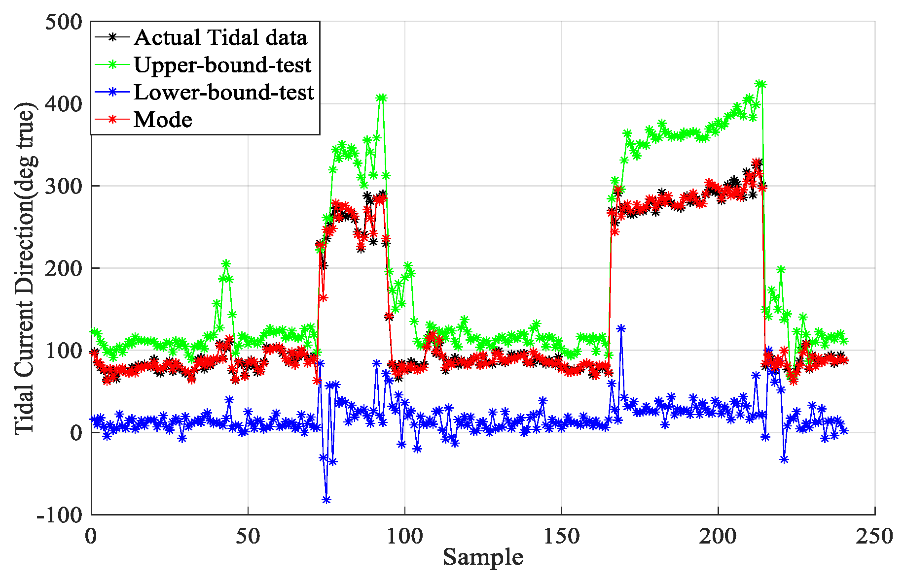
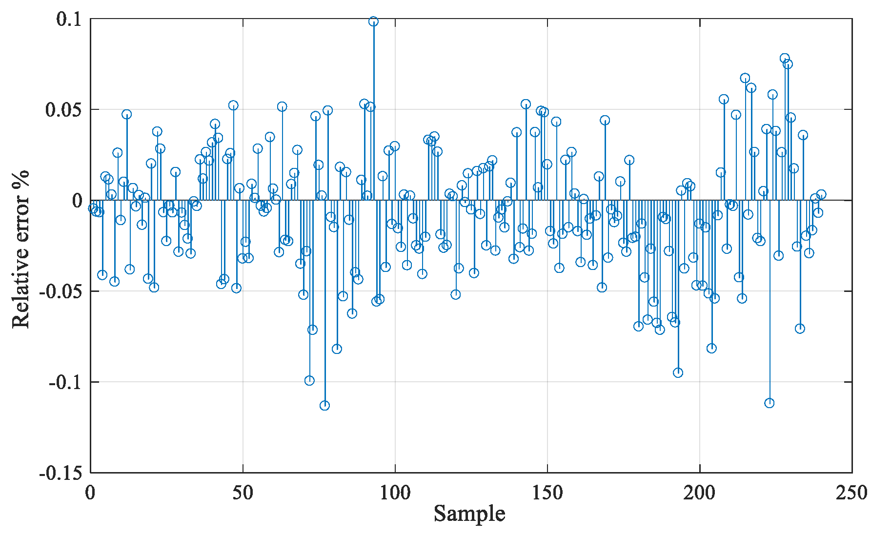
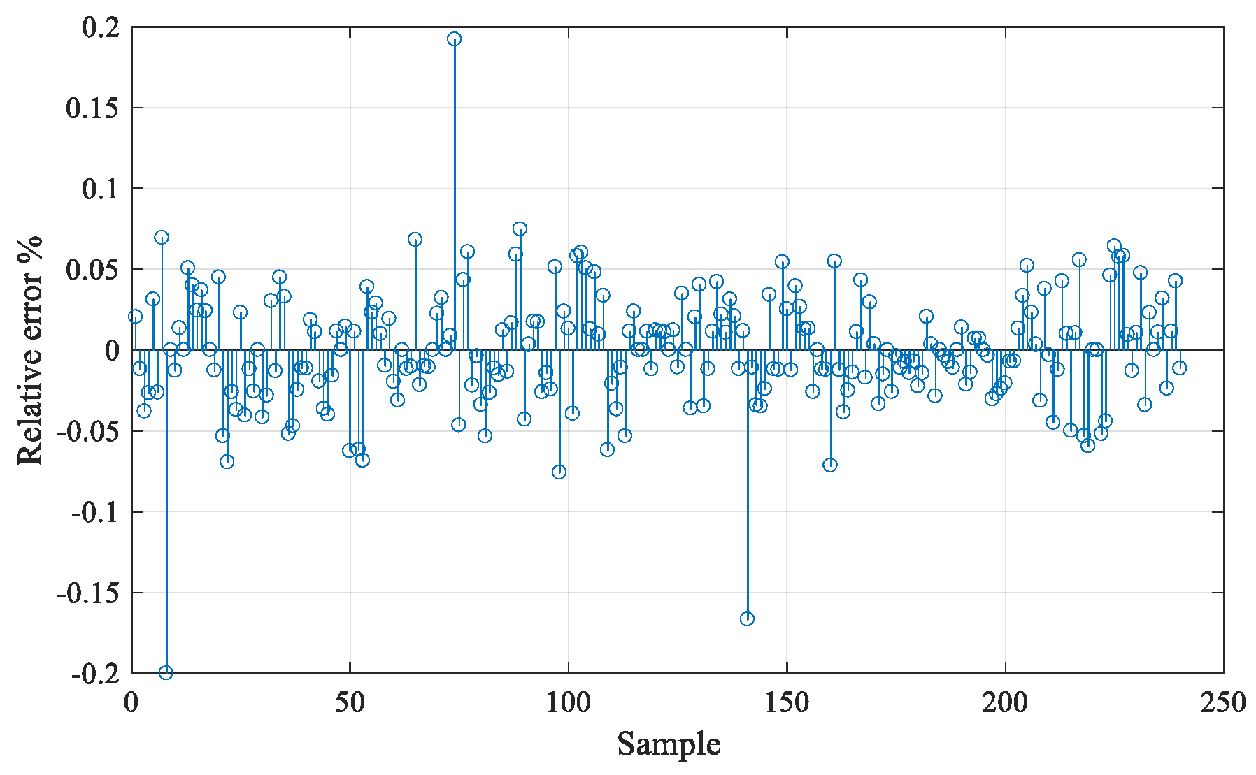
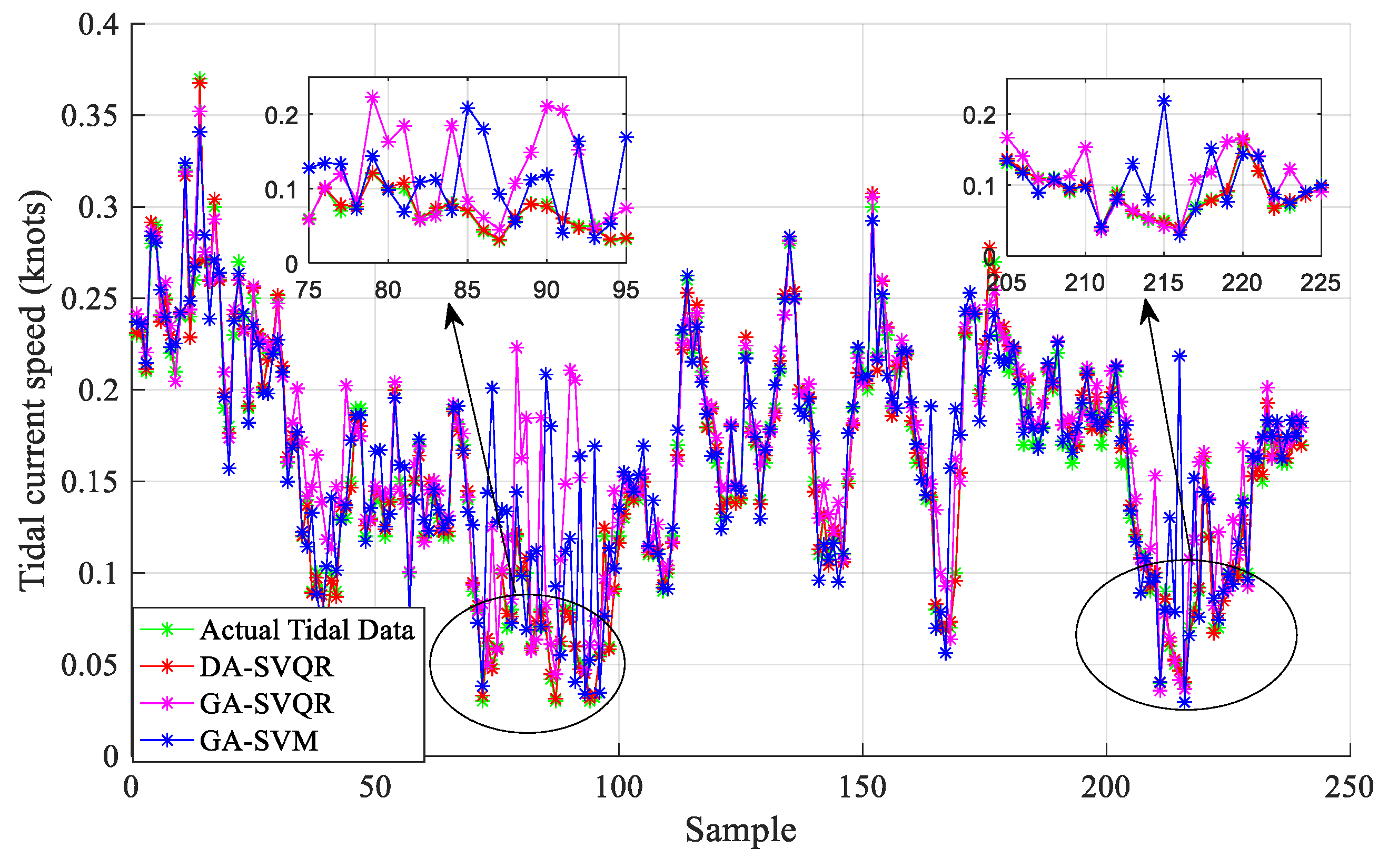
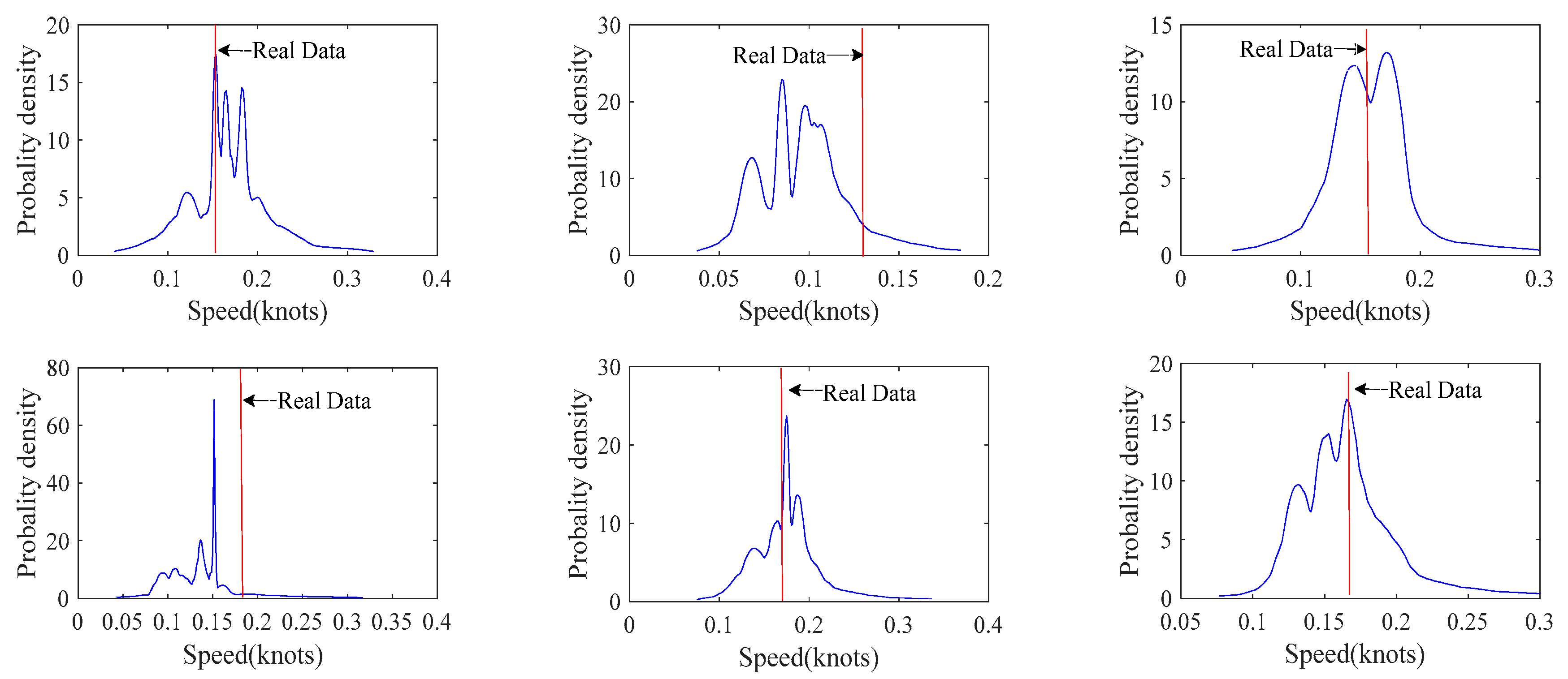
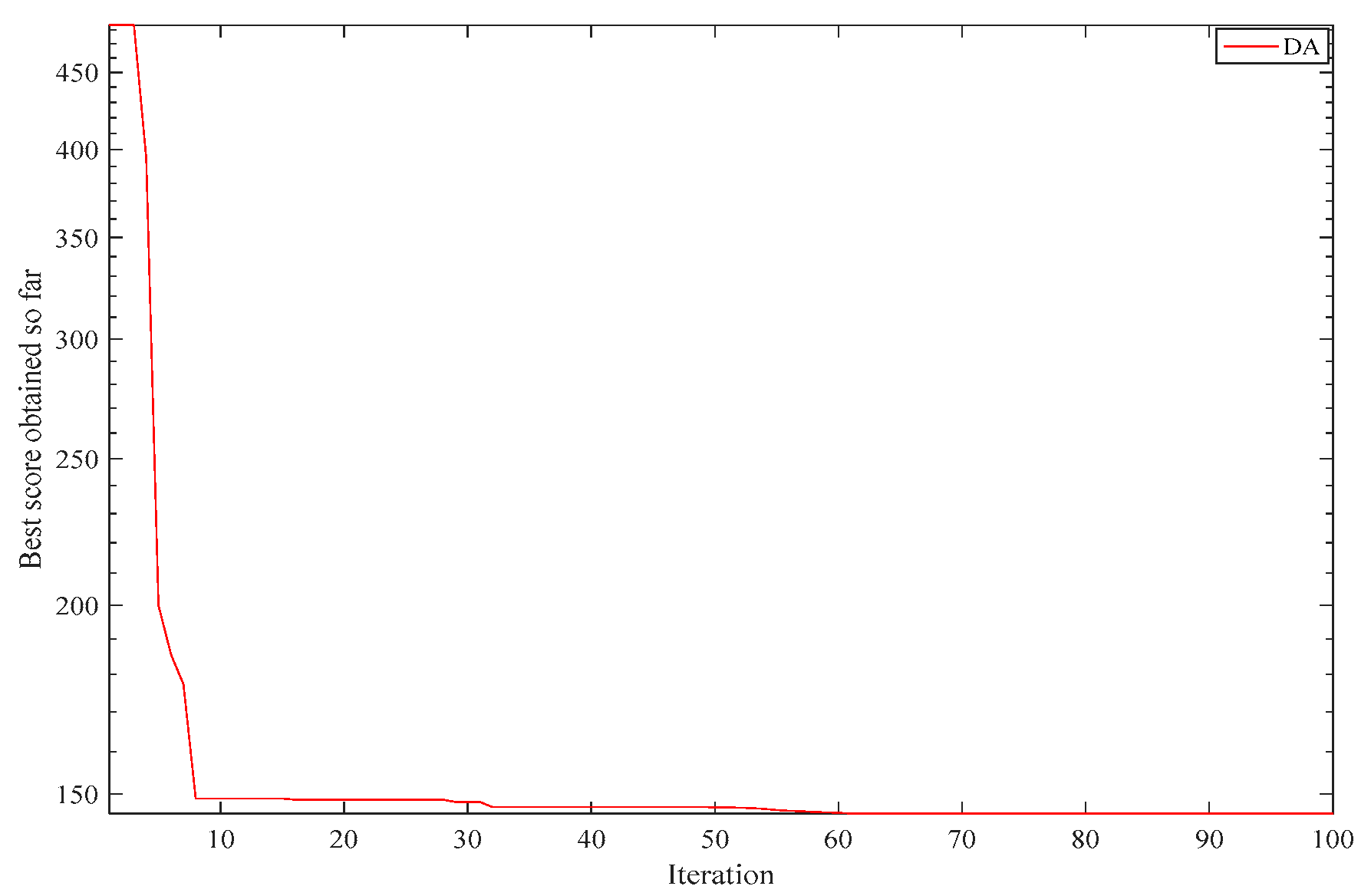
4.1. Analysis of Pradiction Results

As stated above, the DA-SVQR method was used to obtain the tidal current prediction results including prediction interval and probability density curve on day 24 June 2017. Among them, 99 quantiles from 0.01 to 0.99 were selected with a range of 0.01. Figure 4 and Figure 5 show the prediction interval (one point every 6 min) of the tidal current speed and tidal current direction, respectively. Figure 6 and Figure 7 show the predicted relative errors of tidal current speed and tidal current direction, respectively.

It can be observed from Figure 4 and Figure 5 that the actual value initially fell within the prediction interval, and mode (the peak of probability density function) of the prediction result using the DA-SVQR model was very close to the actual value, which illustrates that the DA-SVQR method accurately depicts tidal current fluctuations. It can be seen from Figure 6 and Figure 7 that the relative errors were mostly within 5% indicating that the prediction accuracy was relatively high. Some large relative errors points might be caused by the tidal current changing dramatically. However, when the tidal current changed sharply, the prediction method could still track the trend of the tidal current, which indicates that the proposed method could describe the changes of speed and direction correctly. In Figure 8, the results of SVQR and SVM based on the classical genetic algorithm (GA) are presented. It can be seen that the proposed method could capture the change trend of the actual values better. Figure 9 shows the probability density curves of tidal current speed in the 2nd, 6th, 12th, 16th, 20th and 24th hours respectively. It can be observed that the prediction value of the tidal current speed by the DA-SVQR all appeared on the probability density curve. This result further explained the advantages of the probability density prediction methods in quantifying uncertainty and improving prediction accuracy. In summary, the predicted value and prediction errors obtained by the proposed method could better provide information for decision-makers, provide effective guarantee for the reliability and optimal dispatching strategy of offshore microgrid, and also an effective prediction method for tidal current prediction.

It is more effective to explain the advantages of the DA-SVQR prediction model and the advantages of the DA algorithm in solving the optimization operation problem.

Table 2. Prediction error of dragonfly algorithm (DA)-SVQR, genetic algorithm (GA)-SVQR and GA-support vector regression (SVR) methods.

Method	Evaluation Index
	MAPE%	RMSE%
DA-SVQR	2.8142	1.5069
GA-SVQR	7.2137	2.7217
GA-SVR	10.6869	3.0346

gives the tidal current speed prediction results of the DA-SVQR, GA-SVQR and GA-SVM methods under the same conditions for ten times. As shown in Table 2, the MAPE was 2.8142%, and the RMSE was 1.5069% by the proposed method, which was the minimum among all tests. It indicates that the proposed method had higher stability and higher accuracy against other methods. Moreover, the DA had a better optimization ability and stronger robustness in comparison with the GA.

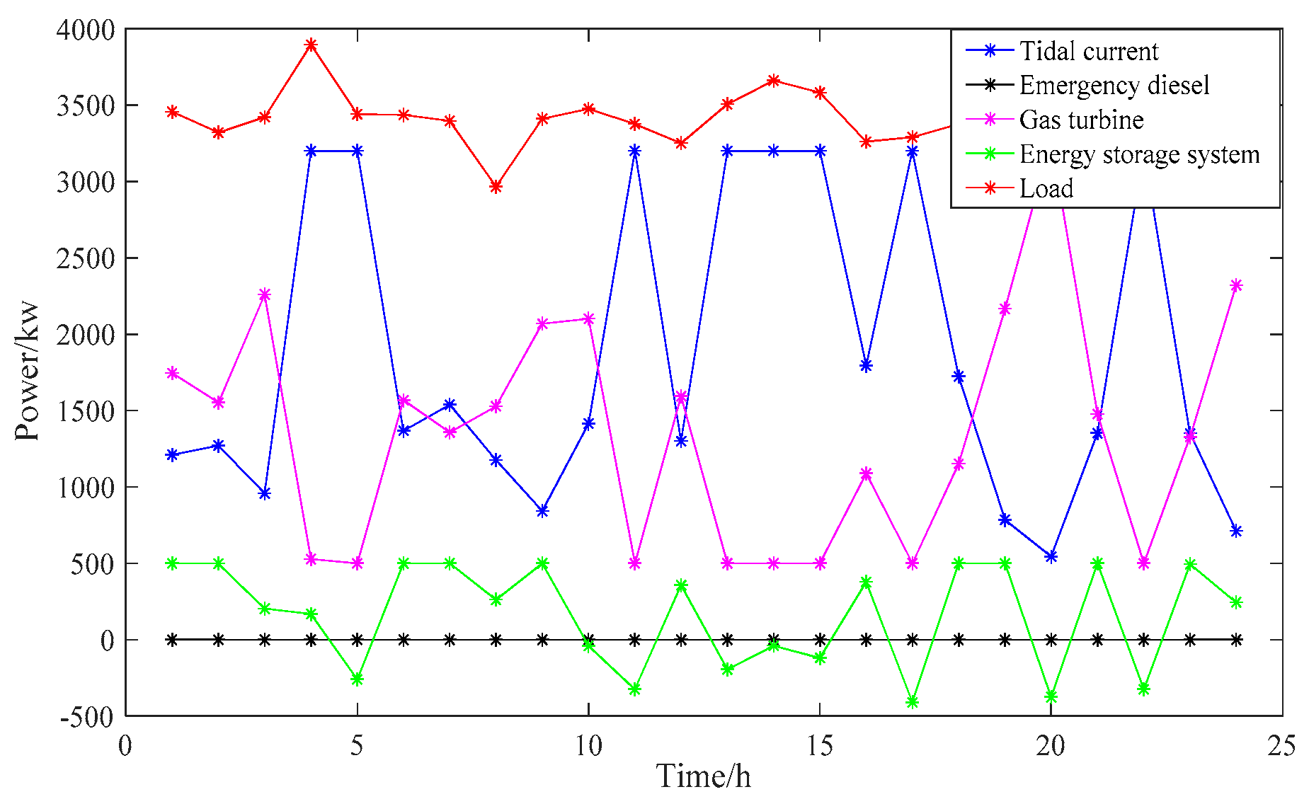
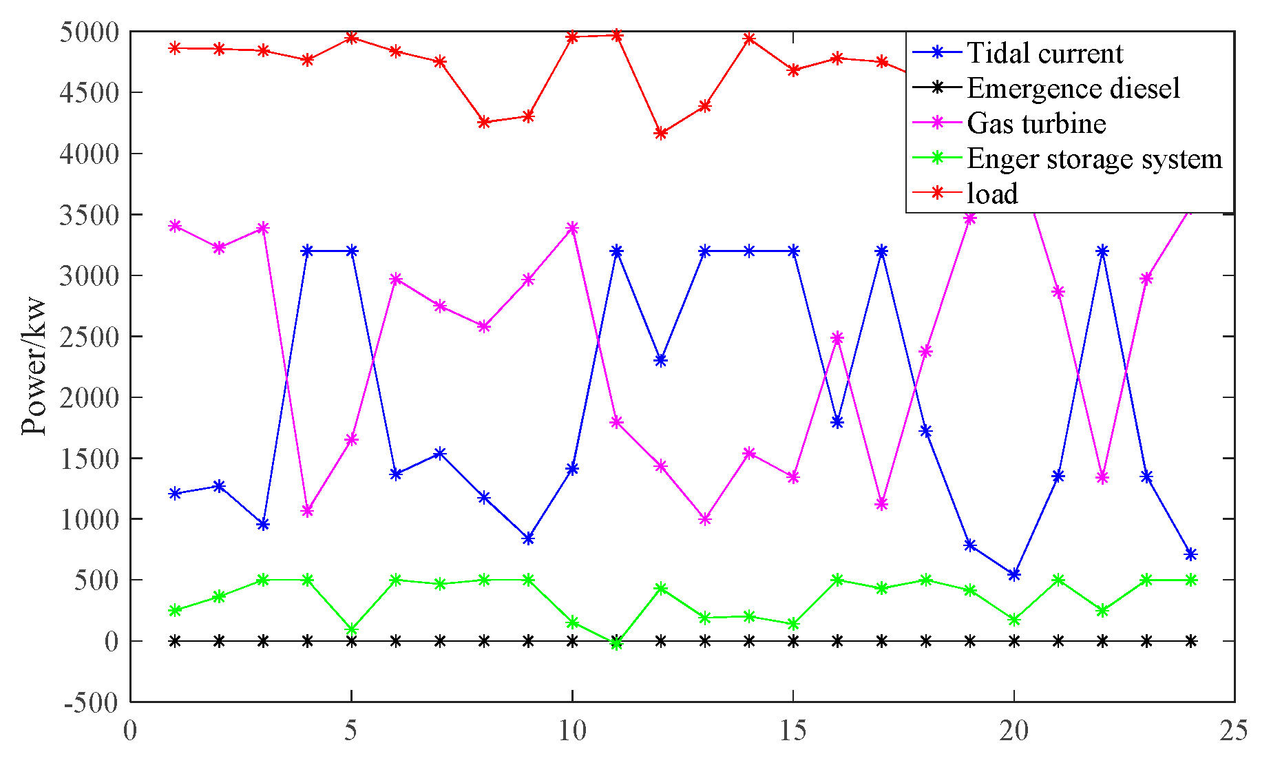
4.2. Analysis of Optimal Dispatching Results

The power output P_out of a tidal current generator can be expressed as (26) [16]:

$$P_{out}=\{\begin{array}{ll}0& 0<V_t<V_{cutin}\\ 0.5C_P\rho A{V}_t^3& V_{cutin}\le V_t<V_{rated}\\ P_{rated}& V_{rated}\le V_t\end{array}.$$

(26)

Here, V_t, V_cutin and V_rated are the tidal current speed, the cut-in speed and the rated speed of the tidal current generator respectively. C_p is the energy capture coefficient of the tidal current generator and ρ is the density of sea water. A is the area swept by the blades of the tidal current generator and P_rated is the rated output power of the tidal current generator.

The parameters of the remaining units of the offshore microgrid are shown in

Table 3. Parameters of each unit of the offshore microgrid.

Device	Parameter	Numerical Value
Energy storage system	Maximum charge and discharge power/kW	50
	Charge and discharge efficiency/%	85
	Battery self-discharge ratio/%	10
	Battery rated capacity (KW*h)	250
	Operation and maintenance cost factor (RMB/KW)	0.02748
Gas turbine	Rated power/KW	200
	Climbing rate/(KW/min)	3
	Minimum operating power	10
	Operation and maintenance cost factor (RMB/KW)	0.03640
	Fuel price (RMB/m3)	27.6
Emergency diesel engine	Upper limit of output power (KW)	100
	Lower limit of output power (KW)	0
	Operation and maintenance cost factor (RMB/KW)	0.0790
	Fuel price (RMB/m3)	38.4
	Single start cost/RMB	100

.

The fuel cost of a gas turbine and emergency diesel engine included transportation cost, storage cost and so on. The fuel prices in the table are the overall prices that take into account the above fees. The problem of the optimal dispatching model for the microgrid can be classified as a multi-objective and nonlinear optimization problem. This paper adopted the dragonfly algorithm to solve the model. Figure 10 shows the power output of each unit in the offshore microgrid in island operation mode.

It can be seen from Figure 10 that during the island operation of the offshore microgrid, the system first used tidal energy, followed by the gas turbine. The emergency diesel engine would not start if there was no special case, which was determined by the economic cost and environmental protection cost in this paper. Moreover, it can be observed in Figure 10 that under the optimization of the algorithm, the energy storage system was charged in the electricity valley and discharged at the electricity consumption peak, which fully reflects the value of cutting peaks, filling the valley and reducing fluctuations. Figure 11 shows that the dragonfly algorithm converged to the optimal value when the iteration reached 50 times, which reflected that the dragonfly algorithm had satisfied convergence speed and less optimization time.

The offshore microgrid in grid-connected mode was employed to verify the effectiveness and correctness of the proposed method under different operation modes, as shown in Figure 12, and the tidal current generators are located in node 21 and node 25. In the dotted frame is a small circular island microgrid, which is connected to another large offshore microgrid to form an offshore microgrid with the grid-connected mode.

Figure 13 shows the power output of each unit in the offshore microgrid under grid-connected operation mode. It can be seen from Figure 13 that the tidal energy was still the priority power and then the gas turbine. Figure 14 shows that the dragonfly algorithm converged to the optimal value when the iteration reached forty-five times. In summary, both in island operation mode or grid-connected operation mode, the optimal dispatching strategy proposed in this paper could make the microgrid run in a more effective and environmentally friendly state.

5. Conclusions

This paper not only proposed a probability prediction method of tidal current based on the support vector quantile regression but also suggests an optimal dispatching strategy for offshore microgrids. By taking the offshore microgrid in the Bohai sea as a case to verify the validity and correctness of the proposed methodology, the following conclusions could be drawn:

It was found that, in all tests, the actual values always fell within the prediction interval obtained by the DA-SVQR, and the results of this method were consistent with the actual curve values. Not only could the way depict the volatility of tidal current correctly but also its results appeared at the mode of the probability density curve with higher probability. The proposed method was effective in quantifying the uncertainty, which would contribute to the increase of the forecasting accuracy of the tidal current.

Moreover, this paper established an offshore microgrid optimization scheduling model considering the tidal current speed prediction, which aimed at minimizing the overall operation cost of the offshore microgrid. The proposed model may improve the operational technology of offshore microgrids and enable the microgrids to achieve better economic and environmental outcomes.

References

1. Zhang, D.; Wang, J. Research on construction and development trend of micro-grid in China. Power Syst. Technol. 2016, 40, 451–458. [Google Scholar]
2. Cai, C.; Liu, H.; Zheng, H.; Chen, F.; Deng, L.; Xu, Q. Microgrid multi-source coordination optimal control based on multi-scenarios analysis. J. Eng. 2017, 13, 1457–1461. [Google Scholar] [CrossRef]
3. Wang, S.; Lam, W.-H.; Cui, Y.; Zhang, T.; Jiang, J.; Sun, C.; Guo, J.; Ma, Y.; Hamill, G. Novel energy coefficient used to predict efflux velocity of tidal current turbine. Energy 2018, 158, 730–745. [Google Scholar] [CrossRef]
4. Neill, S.P.; Vögler, A.; Goward-Brown, A.J.; Baston, S.; Lewis, M.J.; Gillibrand, P.A.; Waldman, S.; Woolf, D.K. The wave and tidal resource of Scotland. Renew. Energy 2017, 114, 3–17. [Google Scholar] [CrossRef]
5. Herman, D.; Gundersen, Z. A novel flexible foil vertical axis turbine for rive ocean and tidal applications. Appl. Energy 2015, 151, 60–66. [Google Scholar]
6. Duverger, E.; Penin, C.; Alexandre, P.; Thiery, F.; Gachon, D.; Talbert, T. Irradiance forecasting for microgrid energy management. In Proceedings of the 2017 IEEE PES Innovative Smart Grid Technologies Conference Europe (ISGT-Europe), Torino, Italy, 26–29 September 2017; pp. 1–6. [Google Scholar]
7. Gu, W.; Wang, Z.; Wu, Z.; Luo, Z.; Tang, Y.; Wang, J. An online optimal dispatch schedule for CCHP microgrids based on model predictive control. IEEE Trans. Smart Grid 2017, 8, 2332–2342. [Google Scholar] [CrossRef]
8. Jahromi, M.J.; Maswood, A.I.; Tseng, K.J. Long term prediction of tidal currents. IEEE Syst. J. 2011, 5, 146–155. [Google Scholar] [CrossRef]
9. Li, Y.; Xie, S.; Wang, B.; He, S.; Huang, D.; He, H.; Qi, H. Unmixing: A new direction from classical tidal harmonic analysis. In Proceedings of the OCEANS 2015—MTS/IEEE Washington, Washington, DC, USA, 19–22 October 2015; pp. 1–5. [Google Scholar]
10. Polagye, B.L.; Epler, J.; Thomson, J. Limits to the predictability of tidal current energy. In Proceedings of the OCEANS 2010 MTS/IEEE SEATTLE, Seattle, WA, USA, 20–23 September 2010; pp. 1–9. [Google Scholar]
11. Chen, H.; Aït-Ahmed, N.; Zaïm, E.H.; Machmoum, M. Marine tidal current systems: State of the art. In Proceedings of the IEEE International Symposium on Industrial Electronics, Hangzhou, China, 28–31 May 2012; pp. 1431–1437. [Google Scholar]
12. Aly, H.H.H.; El-Hawary, M.E. A proposed ANN and FLSM hybrid model for tidal current magnitude and direction forecasting. IEEE J. Ocean. Eng. 2014, 39, 26–31. [Google Scholar] [CrossRef]
13. Kavousi-Fard, A. A hybrid accurate model for tidal current prediction. IEEE Trans. Geosci. Remote Sens. 2017, 55, 112–118. [Google Scholar] [CrossRef]
14. Kavousi-Fard, A.; Su, W. A combined prognostic model based on machine learning for tidal current prediction. IEEE Trans. Geosci. Remote Sens. 2017, 55, 3108–3114. [Google Scholar] [CrossRef]
15. Liu, M.; Li, W.; Billinton, R.; Wang, C.; Yu, J. Modeling tidal current speed using a wakeby distribution. IEEE Trans. Power Syst. 2015, 127, 240–248. [Google Scholar] [CrossRef]
16. Liu, M.; Li, W.; Wang, C.; Billinton, R.; Yu, J. Reliability evaluation of a tidal power generation system considering tidal current speeds. IEEE Trans. Power Syst. 2016, 31, 3179–3188. [Google Scholar] [CrossRef]
17. Liu, M.; Li, W.; Billinton, R.; Wang, C.; Yu, J. Probabilistic modeling of tidal power generation. In Proceedings of the 2015 IEEE Power and Energy Society General Meeting, Denver, CO, USA, 26–30 July 2015; pp. 1–5. [Google Scholar]
18. Ren, Z.; Wang, K.; Li, W.; Jin, L.; Dai, Y. probabilistic power flow analysis of power systems incorporating tidal current generation. IEEE Trans. Sustain. Energy 2017, 8, 1195–1203. [Google Scholar] [CrossRef]
19. Dai, Y.; Ren, Z.; Wang, K.; Li, W.; Li, Z.; Yan, W. Optimal sizing and arrangement of tidal current farm. IEEE Trans. Sustain. Energy 2018, 9, 168–177. [Google Scholar] [CrossRef]
20. Ren, Z.; Wang, Y.; Li, H.; Liu, X.; Wen, Y.; Li, W. A coordinated planning method for micrositing of tidal current turbines and collector system optimization in tidal current farms. IEEE Trans. Power Syst. 2019, 34, 292–302. [Google Scholar] [CrossRef]
21. Liu, G.; Zhu, Y.L.; Jiang, W. Wind-thermal dynamic economic emission dispatch with a hybrid multi-objective algorithm based on wind speed statistical analysis. IET Gener. Transm. Distrib. 2018, 12, 3972–3984. [Google Scholar] [CrossRef]
22. Tchapda, G.Y.G.; Wang, Z.; Sun, Y. Application of improved particle swarm optimization in economic dispatch of power system. In Proceedings of the 2017 10th International Symposium on Computational Intelligence and Design (ISCID), Hangzhou, China, 9–10 December 2017; pp. 500–503. [Google Scholar]
23. Pisei, S.; Choi, J.Y.; Lee, W.P. Optimal power dispatch in multi-microgrid system using particle swarm optimization. Electr. Eng. Technol. 2017, 12, 1329–1339. [Google Scholar]
24. Moghaddam, A.A.; Seifi, A.; Niknam, T. Multi-objective operation management of a renewable MG (micro-grid) with back-up micro-turbine/fuel cell/Battery hybrid power source. Energy 2011, 36, 6490–6507. [Google Scholar] [CrossRef]
25. Rao, R.K.; Srinivas, P.; Divakar, M.S.M.; Venkatesh, G.S.N.M. Artificial bee colony optimization for multi objective economic load dispatch of a modern power system. In Proceedings of the 2016 International Conference on Electrical, Electronics, and Optimization Techniques (ICEEOT), Chennai, India, 3–5 March 2016; pp. 4097–4100. [Google Scholar]
26. Lin, S.; Liu, M.; Li, Q.; Lu, W.; Yan, Y.; Liu, C. Normalised normal constraint algorithm applied to multi-objective security-constrained optimal generation dispatch of large-scale power systems with wind farms and pumped-storage hydroelectric stations. IET Gener. Transm. Distrib. 2017, 11, 1539–1548. [Google Scholar] [CrossRef]
27. Koenker, R.; Bassett, G. Regression quantiles. Econometrica 1978, 46, 33–50. [Google Scholar] [CrossRef]
28. Koenker, R. Quantile Regression; Cambridge University Press: New York, NY, USA, 2015. [Google Scholar]
29. Vapnik, V.N. Statistical Learning Theory; Wiley: New York, NY, USA, 1998. [Google Scholar]
30. Mirialili, S. Dragonfly algorithm: A new meta-heuristic optinization technigue for solving single-objective, discrete, and multiobiective problems. Neural Comput. Appl. 2016, 27, 1053–1073. [Google Scholar] [CrossRef]
Figure 1. Structure diagram of the offshore microgrid.
Energies 12 03384 g001
Figure 2. Flowchart of dragonfly algorithm-support vector quantile regression (DA-SVQR).
Energies 12 03384 g002
Figure 3. Offshore microgrid in island operation mode.
Energies 12 03384 g003
Figure 4. Tidal current speed prediction results.
Energies 12 03384 g004
Figure 5. Tidal current direction prediction results.
Energies 12 03384 g005
Figure 6. Tidal current speed prediction relative error.
Energies 12 03384 g006
Figure 7. Tidal current direction prediction relative error.
Energies 12 03384 g007
Figure 8. Method comparison diagram.
Energies 12 03384 g008
Figure 9. Diagram of the probability density curve.
Energies 12 03384 g009
Figure 10. Power output curve of units in island operation mode.
Energies 12 03384 g010
Figure 11. Iterative result diagram of dragonfly algorithms in island operation mode.
Energies 12 03384 g011
Figure 12. Offshore microgrid in grid-connected operation mode.
Energies 12 03384 g012
Figure 13. Power output curve of units in grid-connected operation mode.
Energies 12 03384 g013
Figure 14. Iterative result diagram of dragonfly algorithms in grid-connected operation mode.
Energies 12 03384 g014