Short-Term Load Forecasting for CCHP Systems Considering the Correlation between Heating, Gas and Electrical Loads Based on Deep Learning

Abstract

Combined cooling, heating, and power (CCHP) systems is a distributed energy system that uses the power station or heat engine to generate electricity and useful heat simultaneously. Due to its wide range of advantages including efficiency, ecological, and financial, the CCHP will be the main direction of the integrated system. The accurate prediction of heating, gas, and electrical loads plays an essential role in energy management in CCHP systems. This paper combined long short-term memory (LSTM) network and convolutional neural network (CNN) to design a novel hybrid neural network for short-term loads forecasting considering their correlation. Pearson correlation coefficient will be utilized to measure the temporal correlation between current load and historical loads, and analyze the coupling between heating, gas and electrical loads. The dropout technique is proposed to solve the over-fitting of the network due to the lack of data diversity and network parameter redundancy. The case study shows that considering the coupling between heating, gas and electrical loads can effectively improve the forecasting accuracy, the performance of the proposed approach is better than that of the traditional methods.

1. Introduction

With the rapid development of industry, the consumption of energy and other natural resources has increased substantially. How to rationally utilize energy resources and improve the efficiency of energy utilization has become a common concern of all countries in the world. The combined cooling heating, and power system is one of the distributed energy systems, which uses a power station or heat engine to generate useful heat and electricity at the same time. It is arranged near the users on a small scale, decentralized, and targeted manner, and delivers heating energy and electric energy to nearby users according to the users’ different needs [1,2]. Compared with conventional centralized power systems, the combined cooling, heating, and power (CCHP) system has lower energy costs, higher energy efficiency, and higher energy availability. Therefore, the CCHP system will become the main form of the integrated energy system [3].

The traditional power system, heating system, and natural gas system are independent of each other, which greatly limits the operating efficiency of these three energy systems. The CCHP system uses gas as an energy source and recycles hot water and high-temperature exhaust gas to improve the comprehensive utilization efficiency of energy [4]. In this case, the power system, heating system, and natural gas system will have a strong correlation, which requires the intelligent control of these three systems at the same time. Accurate prediction of heating, gas, and electrical loads is the basic premise of energy management in CCHP systems and has important theoretical and practical value.

Conventionally, heating, gas and electrical loads forecasting are conducted separately, and this is not suitable for CCHP system where the heating, gas, and electrical loads have strong correlations. Therefore, it is necessary to propose a novel load forecasting approach for the CCHP system that accounts for the correlation of these three loads.

Recently, as an important branch of the field of artificial intelligence, the deep learning technology, has been applied to all popular artificial intelligence areas, including speech recognition, image recognition, big data analysis, etc. [5,6,7]. Especially, the convolutional neural network (CNN), which is well-known for its strong ability to extract features, has gained enormous attention in the field of image classification and image recognition. The CNN with global spatial information was designed to divide white matter hyperintensities in [8]. To realize image classification, the CNN with five convolutional layers and three fully connected layers was designed to improve the accuracy in [9]. The phase-functioned network, a maximum posteriori framework and a local regression model were proposed respectively to control real-time data-driven character such as human locomotion in [10,11,12]. Heungil et al. combined the hidden Markov model and automatic encoder to model the underlying functional dynamics inherent in rs-fMRI [13]. At present, the application of CNN on the regression task is very limited. In addition, the long short-term memory network is often used to process time series, for it can establish the correlation between the previous information and the current circumstances [14,15]. To the best of our knowledge, there is no report about combining CNN and LSTM network to predict heating, gas, and electrical loads while considering their correlation.

In this paper, we aim to forecast heating, gas, and electrical loads by combining CNN and LSTM network. Firstly, the Pearson correlation coefficient will be utilized to analyze the temporal correlation between historical loads and current loads, which give the reason for using the LSTM network. Then, a deep learning method composed of CNN and LSTM network could be designed. In addition, the dropout layer is proposed to handle the over-fitting. Finally, the real-world data of CCHP system is used to test the performance of our proposed approaches.

The rest of this paper is organized as follows. Section 2 provides the background of load forecasting. Section 3 analyzes the temporal correlation of the three loads and the coupling between them, and then explains why LSTM should be added to the proposed network. Section 4 introduces the Conv1D, MaxPooling1D, dropout and LSTM layers for load forecasting. Section 5 tests the performance of our proposed approaches and analyses results. Section 6 summaries the conclusions.

2. Literature Review

Heating, gas, and electrical loads forecasting are essential to CCHP systems planning and operations. In respect of time horizons, the loads forecasting can be roughly split into long-term load forecasting, medium-term load forecasting, short-term load forecasting, and very short-term load forecasting, among which the predicted time horizon cut-offs are years, months, hours, and minutes, respectively. This section will provide a brief review of short-term load forecasting.

In the previous literature, several forecasting approaches were proposed for predicting heating, gas, and electrical loads. The conventional methods mainly include autoregressive integrated moving average (ARIMA), model support vector machine (SVM), regression analysis, grey theory (i.e., GM (1,1)) and artificial neural network (ANN).

The current state of heating, gas, and electrical loads is not only related to the surrounding environmental factors but also influenced by past events. The ARIMA and GM (1,1) models predict current load according to historical time series, which can fully consider the trend and transient state. However, they ignore environmental factors. Therefore, when the surrounding environment changes dramatically, the historical trend of the load is not smooth, and the error of these methods may become very large [16,17].

Regression analysis fits the given mathematical formula based on historical data, but it has the drawback that the relationship between loads and features is difficult to be accurately described by a mathematical formula [18]. In the field of computer science, SVM is a supervised learning model, which is often utilized for the task of classification and regression analysis. It is good at solving a large number of complex problems, such as nonlinear, over-fitting, high dimension, and local minimum point. However, the SVM has a slow speed of training large-scale samples [19,20]. As a “black-box” that relies on data and prior knowledge, the traditional ANN can fit complex nonlinear relationships, whereas the traditional ANN also has defects of over-fitting and easy to fall into local optimum [21,22]. In addition, the above methods only account for the impact of the environmental factors on the current loads, ignoring the role of past events.

Recently, the deep learning network has been applied to forecast heating, gas and electrical loads. The deep belief network is designed to forecast day-ahead electricity consumption in [23]. The study cases show that the proposed approach is suitable for short-term electrical load forecasting. In addition, it offers better results than traditional methods. Indeed, the LSTM is good at dealing with time series with long time spans, which is suitable for forecasting short-time loads. Kuan Lu et al. proposed a concatenated LSTM architecture for forecasting heating loads [24]. In order to solve the forecasting problem for the strong fluctuating household load, Weicong Kong et al. improved the household prediction framework with automatic hyper parameter tuning based on LSTM network [14]. The CNN is a neural network designed to process input data that has an intrinsic relationship. Generally, the input data to CNN will have a natural structure to it such that nearby entries are correlated [25,26]. For example, this type of data includes 1-D load time series and 2-D images. The current research mainly focuses on 2-D image recognition. The literature about using CNN to extract the features of time series for forecasting loads is relatively limited. In order to improve the performance of the network, researchers try to combine CNN with LSTM to form a hybrid network. A CNN-LSTM neural network is proposed to extract temporal and spatial features to improve the forecasting accuracy of household load in [27]. Jianfeng et al., designed a hybrid network consisting of the CNN and LSTM to improve the performance of recognizing speech emotion [28]. Similarly, The CNN and LSTM are utilized to automatically detect diabetes in [29]. At present, there is no report on the use of hybrid network consisting of the CNN and LSTM to predict heating, gas, and electrical loads while considering the correlation of these three loads for integrated energy systems.

In addition, previous studies show that the performance of multi-layer is better than that of single-layer for all of the above deep learning models. However, some scholars have found that over-fitting occurs as the number of layers increases. [30,31]. Therefore, it is necessary to find a way that can increase the number of layers without over-fitting.

Taking the above analysis into consideration, it is clear that though the predecessors have made great achievements in heating, gas and electrical loads forecasting, there are still some problems to be solved. For example, how to combine CNN and LSTM to design a hybrid network, which can not only extract the inherent features of the input but also consider the temporal correlation of loads? How to solve the over-fitting? How does the coupling between heating, gas, and electrical loads affect the forecasting results?

To solve these problems for heating, gas, and electrical loads forecasting, a new framework based on deep learning is proposed. The key contributions of this paper can be summarized as follows:

(1)

The heating, gas, and electrical loads of the CCHP system are highly coupled. Although there is a lot of literature focusing on load forecasting, the prediction of multiple loads considering their coupling has not been found in the literature. This is the first time to design a network to forecast loads, considering the coupling between them.

(2)

Pearson correlation coefficient will be utilized to measure the temporal correlation between historical loads and current loads, to give the reason for using the LSTM network.

(3)

The Conv1D layer and MaxPooling1D layer are utilized to inherent features that affect heating, gas, and electrical loads. To prevent over-fitting, the dropout is added between LSTM layers. The LSTM network which could take the influence of previous information into account is adopted to forecast these loads.

3. Analysis of Temporal Correlation

As we all know, loads have temporal correlations, especially electrical loads. For example, if the air conditioner is turned on at the moment, the air conditioning load will continue for some time in the future. Furthermore, there are many methods, such as the GM (1,1) model, that predict next loads based on the trend of historical load series. In the past, heating, gas, and electrical loads systems operated independently and their coupling was not strong. Therefore, few people study the temporal correlation between multiple loads. The heating, gas, and electrical loads can be converted in real-time through related devices in CCHP systems, which lead to a strong temporal correlation of these three loads.

Pearson correlation coefficient whose value ranges from −1 to +1 is able to measure the linear correlation of two variables. In this paper, the Pearson coefficient will be utilized to evaluate the temporal correlation of these three loads. The Pearson correlation coefficient can be expressed as follows [32]:

$$r_{xy}=\frac{{\displaystyle \sum _{i=1}^n(x_i-\overline{x})(y_i-\overline{y})}}{\sqrt{{\displaystyle \sum _{i=1}^n{(x_i-\overline{x})}^2}}\sqrt{{\displaystyle \sum _{i=1}^n{(y_i-\overline{y})}^2}}}$$

(1)

where $\overline{x}$ stands for the mean of $x$ and $\overline{y}$ stands for the mean of y.

In this study, the dataset comes from a hospital in Beijing, China, which contains hourly data from 1 January, 2015 to 31 December, 2015. The main features include environmental factors, such as moisture content, humidifying capacity, dry bulb temperature, and total radiation. The Pearson coefficient is used to analyze the relationship between current heating, gas, and electrical load (loads at time t) and their historical loads (loads from t-24 to t-1). The results are shown in Figure 1.

On one hand, the Pearson coefficient between the current heating loads and the historical heating loads is large, i.e., the heating load itself has a strong temporal correlation. In addition, the Pearson coefficients between the heating loads and the electrical loads and the gas loads are small, which indicates that there is weak coupling between heating loads and the other two kinds of loads. On the other hand, both the gas load and the electrical load have strong coupling with themselves. Besides, there is a strong coupling between the current gas load and the historical electrical load which ranges from t-1 to t-5. Electrical loads also have a similar conclusion that there is a strong coupling between the current electrical load and the historical gas load which ranges from t-1 to t-4.

As can be seen from the above simulation, the heating, gas, and electrical loads have strong temporal correlation and coupling, which requires the deep learning network to consider these factors.

4. Deep Learning Framework for Forecast Short-Term Loads

4.1. Conv1D Layer and MaxPooling1D Layer

CNN is a neural network designed for processing input data that has an intrinsic relationship. For example, a time series can be thought of as a one-dimensional grid sampled at fixed time intervals, and image data can be viewed as a two-dimensional grid of pixels [33]. CNN has been widely used in image recognition tasks with good performance. As the name implies, the main mathematical operation of convolution neural networks is convolution that is a special linear operation. The matrix multiplication is replaced by convolution layers in CNN.

As is known to all, the convolution is a mathematical operation on two functions of a real-valued argument. The convolution operation can be described as follows:

$$s=x\ast w$$

(2)

where w stands for the weighting function which is called kernel in CNN. x stands for the input function. The output of convolution can be marked as s, which will be called the feature map. $\ast$ represents the operation of convolution.

In practical problems such as load forecasting, the data of input is a multiple dimensional vector, and the kernel is also a multiply dimensional vector of parameters which are determined by learning method. In this case, the operation of convolution will be applied to multiple dimensions since the kernels and inputs are multiple dimensional. Therefore, the operation of convolution for two-dimensional inputs can be described as follows:

$$s(i,j)=(I\ast K)(i,j)={\displaystyle \sum _l{\displaystyle \sum _{m}I(l,m)K(i+l,j+m)}}$$

(3)

where I is the two-dimensional data of input, and K is the two-dimensional kernel. S represents the feature map after the operation of convolution.

As shown in Figure 2, a typical CNN consists of a set of layers. The input layer is composed of environmental factors and historical loads. Assuming that the dimension of the input layer is 28, five feature maps are generated after convolution operation. The pooling layers are often inserted between the Conv1D layers. It effectively alleviates over-fitting by reducing the parameters between layers. According to the conclusion from the literature [24], the computationally efficient max pooling showed better results than other candidates, including average pooling and min pooling. The MaxPooling1D layer resizes it spatially and operates on every depth slice of the data.

Generally speaking, the neural network includes one or more Conv1D and MaxPooling1D layers. After extracting features by using Conv1D and MaxPooling1D layers, the outputs will be sent to LSTM layers.

4.2. LSTM Layer

The recurrent neural network (RNN) is a typical artificial neural network that establishes the temporal correlations between the current circumstances and previous information [34]. Unlike traditional feed forward neural network, the RNN can use their internal memory to process time series of input data. Such characteristic of RNN makes it applicable to load forecasting, because the heating, gas, and electrical loads are affected by environmental features and historical loads.

The common training approaches for RNN mainly include real-time recurrent learning (RTTL) and back propagation through time (BPTT). Compared with RTRL, The BPTT algorithm has a shorter computation time [35]. Therefore, BPTT is often used to train RNN. Because the problems of gradient vanishing and gradient exploding, learning long-range dependencies with RNN is difficult. These problems limit the ability to learn temporal correlations of long-term time series. The long short-term memory (LSTM) was proposed by Hochreiter to solve these problems in 1997 [36]. Broadly speaking, LSTM is one of the RNNs. It not only has memory and forgetting patterns to learn the features of time series flexibly, but also solves the problem of gradient exploding and gradient vanishing. Recently, LSTM networks have achieved great success in numerous sequence prediction tasks, which include speech prediction, handwritten text prediction, etc. Figure 3 shows the block structure of LSTM at a single time step.

The cell state vector $c_t$ is read and modified through the control of forget gate $f_t$, input gate $i_t$ and output gates $o_t$ during the whole life cycle, which is the most important structure of the LSTM layer. The current cell state vector $c_t$ will be determined by operating the output vector $h_{t-1}$, input vector $x_t$ and previous cell state vector $c_{t-1}$ according to the present time steps and the outputs of the previous time step. The formula for the relationship between the variables is as follows:

$$f_t={\sigma }_g(W_f{x}_t+U_f{h}_{t-1}+b_f)$$

(4)

$$i_t={\sigma }_g(W_i{x}_t+U_i{h}_{t-1}+b_i)$$

(5)

$$o_t={\sigma }_g(W_o{x}_t+U_o{h}_{t-1}+b_o)$$

(6)

$$c_t=f_t\circ c_{t-1}+i_t\circ {\sigma }_c(W_c{x}_t+U_c{h}_{t-1}+b_c)$$

(7)

$$h_t=o_t\circ {\sigma }_c(c_t)$$

(8)

where $W\in R^{n\times d}$ are the weight matrices. $U\in R^{n\times n}$ are bias vector parameters. The superscripts n is the number of hidden units and d is the number of input features. ${\sigma }_c$ is hyperbolic tangent functions and ${\sigma }_g$ is the sigmoid function.

The hyperparameter of the hidden unit n should be specified to train the LSTM network. Therefore, the output vector $h_t$ and cell state vector $c_t$ are n-dimensional vectors, which are equal to 0 at the initial time. The LSTM has three sigmoid functions whose output data range from 0 to 1. They are usually regarded as "soft" switches to determine which data should pass through the gate. The signal will be blocked by the gate when the gate is equal to 0. The states of input gate $i_t$, output gate $o_t$ and forget gate $f_t$ all rely on previous output $h_{t-1}$ and the current input $x_t$. The signal of forget gate determines what to forget of the previous state $c_{t-1}$, and the input gate decides what will be preserved in the internal state $c_t$. After updating the internal state, the output data of LSTM will be determined by the internal state. Similarly, this process will be repeated for the next time steps. In general, the LSTM output of the next time steps can be affected by the information of the previous time steps through this block structure of LSTM.

4.3. Dropout Layer

Previous studies have shown that increasing the number of layers in the neural network does not effectively improve forecasting accuracy. The number of internal parameters of the network increases exponentially when the number of network layers increases. It is prone to over-fitting. After training the network, the network will be created perfectly, but just for the training set. Dropout is a technique that addresses over-fitting [37,38]. As shown in Figure 4, some units are selected randomly and their incoming and outgoing connections are discarded from the network. At each training phase, each unit "exits" the network with a probability p to reduce the parameters of the network. Only the reduced network will be trained in the stage, and the removed units will be reinserted into the network with their original weights.

The probability of discarding hidden units is set to 0.5. In term of input units, the probability should be much lower because if the input units are ignored, the information will be lost directly. By avoiding training all units of the network, the dropout layer can decrease over-fitting. Especially for deep neural networks, dropout technique can significantly shorten the training time.

4.4. Framework for Multiple Loads Forecasting Based Deep Learning

Figure 5 shows the framework of short-term loads forecasting based on deep learning. The process of load forecasting is as follows:

(1)

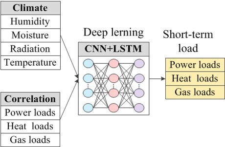
The input data include historical loads and environmental factors such as moisture content, humidifying capacity, dry bulb temperature, and total radiation. The min-max normalization is used to bring all input data into the range from 0 to 1.

(2)

Next step is to determine the structure of network and parameters, such as the number of LSTM layer, the number of unit in each LSTM layer, the number of CNN layer, the size of kernel weight, the size of pooling, epochs and the size of each batch.

(3)

The input data will be sent to Conv1D layers. The MaxPooling1D layer is added between the two Conv1D layers. It extracts the maximum value of the filters and provides useful features while reducing computational cost thanks to data reduction.

(4)

In the LSTM layer, the time steps are sent to relevant LSTM block. The number of LSTM layers can be revised arbitrarily because of the sequential character of the output of the LSTM layer.

The output data of the LSTM layer are used as input of the full connection layer, and the predicted load is output by the full connection layer.

After designing the structure of the neural network, it is necessary to determine the training method. Now, the main training methods of recurrent neural networks, such as LSTM, include real-time recurrent learning (RTRL) and back propagation through time (BPTT). Compared with BPTT, RTRL has lower computational efficiency and longer computing time [33]. Hence, the proposed network will be trained by BPTT. Moreover, previous research suggests Adam approach can achieve better performance than other optimizers, such as Adagrad, Adadelta, RMSProp, and SGD [34]. Therefore, the optimizer for the training proposed approach is Adam. The loss function is MAE.

The main steps of the proposed method can be summarized as follows: (1) Define the CNN-LSTM network, (2) compile the CNN-LSTM network, (3) fit the CNN-LSTM network, (4) predict the loads. The part of the code for the proposed method is shown in

Table 1. The code for the proposed method.

Program: A part of codes for building the CNN-LSTM network

#1 Define the CNN-LSTM Network model = Sequential() model.add(Conv1D(filters=10, kernel_size=3, padding=’same’, strides=1, activation=’relu’,input_shape=(1, Input_num))); model.add(MaxPooling1D(pool_size=2)) model.add(Dropout(rate=0.25)) model.add(Conv1D(filters=20, kernel_size=3, padding=’same’, strides=1, activation=’relu’)) model.add(MaxPooling1D(pool_size=2)) model.add(Dropout(rate=0.25)) model.add(LSTM(units=24,return_sequences=True)) model.add(LSTM(units=16,return_sequences=True)) model.add(LSTM(units=32,return_sequences=True)) model.add(LSTM(units=16,return_sequences=True)) model.add(LSTM(units=16,return_sequences=True)) model.add(LSTM(units=16)) model.add(Dense(units=1, kernel_initializer=’normal’,activation=’sigmoid’)) #2 Compile the CNN-LSTM network model.compile(loss=’mae’, optimizer=’adam’) #3 Fit the CNN-LSTM network history = model.fit(trainX,trainY, epochs=100, batch_size=50,validation_data=(valid3DX, validY), verbose=2, shuffle=False) #4 Predict the loads Predicted_Load = model.predict(testX)

.

4.5. Indicators for Evaluating Result

To measure the predictive effect from various perspectives, mean absolute percentage error (MAPE) will be adopted in this paper. The mathematical formula is as follows:

$$MAPE=\frac{1}{n}{\displaystyle \sum _{i=1}^n\left|\frac{{\hat{y}}_i-y_i}{y_i}\right|}$$

(9)

where n stands for the number of test sets. ${\hat{y}}_i$ is the forecasting load and $y_i$ is the real load.

5. Case Study

5.1. Experimental Environment and Parameters

The dataset comes from a hospital in Beijing, China, which contains 8760 samples from 1 January 2015 to 31 December 2015. The sample interval was one hour. The loads and corresponding features from 1 January 2015 to 19 October 2015 were used for the training set and the data from 20 October 2015 to 25 November 2015 were used for the validation set. The other data were considered as testing data. The equipment of the integrated energy system mainly included gas boiler, gas-combustion generator, waste-heat recovery system, electric refrigeration unit, lithium bromide refrigeration unit, storage battery and heat storage system. All the proposed methods were conducted using Keras on a notebook computer equipped with Intel (R) Core (TM) i5-6500 CPU @ 3.20 GHz processor and 8 GB of RAM.

In order to verify the validity of the proposed algorithm, the proposed algorithm was compared with the traditional methods (BP network, ARIMA, SVM, LSTM, CNN). The parameters of each algorithm were tested several times in order to achieve optimal performance. However, not all results will be shown here. After many trials, the optimal structure and parameters of each algorithm arweree set as follows:

BP network: The epochs were set to 100. The middle layer consisted of two fully connected layers with 10 and 15 neurons respectively.

ARIMA: The degree of difference was two and the number of autoregressive terms was four. The number of lagged forecast errors was four.

SVM: The kernel function of SVM used the radial basis function (RBF).

LSTM: The neurons’ number in the input layer equaled the number of features, and the neurons’ number in the output layer was 1. After many trials, the best choice was to use six LSTM layers. The neurons’ number in each layer was 32, 16, 32, 16, 16, and 8, respectively.

CNN: After many trials, the best solution of CNN was to use two Conv1D layer and MaxPooling1D layer. The filters were 10 and kernel size was three in the first Conv1D layer. The filters were 20 and kernel size was three in the second Conv1D layer. Both pool sizes of MaxPooling1D were equal to two.

CNN-LSTM: After many trials, the best solution of CNN was to use two Conv1D layer and MaxPooling1D layer. The filters were 10 and kernel size was three in the first Conv1D layer. The filters were 20 and kernel size was threw in the second Conv1D layer. Both pool sizes of MaxPooling1D were equal to two. The best choice was to use six LSTM layers. The neurons’ number in each layer was 24, 16, 32, 16, 16, and 16, respectively. Both rates of the dropout were set to 0.25.

This section mainly consists of the following four points: (1) The performance for forecasting heating, gas, and electrical loads was tested in different time steps, (2) the influence of the coupling of heating, gas, and electrical loads on the accuracy of prediction was analyzed, (3) the relationship between the forecasting results and the layers’ number of the network is explored, and the influence of the dropout layer on the forecasting accuracy were analyzed, (4) the performance of proposed approaches is compared to traditional methods to validate the efficacy.

5.2. Performance in Different Time Steps

The LSTM network forecasts the loads by using the environmental factors and historical load series whose length can be changed arbitrarily theoretically. If the time steps of power load are too short, it may lead to the insufficiency of learning historical trend. In contrast, if the time steps of power load are too long, it may aggravate the complexity of the proposed methods, which may make the accuracy worse.

To explore how many historical load series are applied to LSTM network for forecasting loads, multiple cases with different time steps which range from 0 to 10 were tested. The average MAPE was calculated by testing the data set 50 times independently. Figure 6, Figure 7 and Figure 8 show the result of MAPE in different time steps.

As the time steps increase, the overall trend of the heating load of MAPE decreases. This phenomenon suggests that there is a strong temporal correlation between the current heat load and the historical heat load from t-1 to t-10, which is consistent with the conclusions drawn in Figure 1 above. The current gas and electrical loads also have a strong temporal correlation with historical loads from t-1 to t-2, and a weak temporal with historical loads from t-3 to t-10. In this data set, two look-back time steps can achieve the best accuracy for forecasting gas and electrical loads.

When time steps are equal to 0, the MAPE of the heating, gas, and electrical loads are equal to 0.145, 0.158, and 0.143, respectively. In general, considering historical load series can significantly reduce the error for predicting heating, gas, and electrical loads. It shows the need to find a network that can account for temporal correlations to predict heating, gas, and electrical loads, which explains why the LSTM layer is used in the proposed approach.

5.3. The Influence of the Coupling of Heating, Gas and Electrical Loads on the Results

To analyze the impact of the coupling of heating, gas and electrical loads on the forecasting results, eight cases, as shown in

Table 2. Different case for simulation.

Scenes	Input of Network
Case 1	Environmental features
Case 2	Environmental Feature, heating loads
Case 3	Environmental features, gas loads
Case 4	Environmental features, electrical loads
Case 5	Environmental feature heating and gas loads
Case 6	Environmental features heating and electrical loads
Case 7	Environmental features gas and electrical loads
Case 8	Environmental features heating, gas and electrical loads

, were designed for simulation. Each case ran 50 times independently to obtain the average MAPE, and the result is shown in

Table 3. The average MAPE of heating loads.

Scenes	Case 1	Case 2	Case 5	Case 6	Case 8
MAPE	0.145	0.057	0.065	0.062	0.073

,

Table 4. The average MAPE of gas loads.

Scenes	Case 1	Case 3	Case 5	Case 7	Case 8
MAPE	0.158	0.060	0.772	0.055	0.064

and

Table 5. The average MAPE of electrical loads.

Scenes	Case 1	Case 4	Case 6	Case 7	Case 8
MAPE	0.143	0.086	0.092	0.083	0.085

.

The results in Table 3, Table 4 and Table 5 indicate that:

(1)

In terms of heating loads, it is obvious that the forecasting accuracy of Case 2 is higher than that of Case 1, which reveals that the heating loads have a strong temporal correlation and considering temporal correlation helps improve the accuracy of the prediction. By comparing the MAPE of Case 1 and Case 2, it is found that taking the gas load as input will reduce the accuracy for forecasting heating load. Similarly, the conclusion is the same for heating load and electrical load. This is because the coupling between the heating load and the other loads is weak, which is consistent with the conclusions of the previous analysis. The addition of the gas load and the electrical load will interfere with features of the input, which makes the accuracy of the prediction worse.

(2)

As far as gas load is concerned, it can be found from Case 3 that the gas load also has a strong temporal correlation. Compared with Case 3 and Case 5, it is evident that the correlation between gas load and heating load is very weak. The input of heating load will lead to a decrease in forecasting accuracy of gas load. On the contrary, the coupling between gas load and electrical load is very strong. Adding electrical load as input is helpful to improve accuracy.

(3)

The result of Case 4 from Table 4 shows that there is a strong temporal of electrical load. The input of heating load will lead to a decrease in forecasting accuracy of electrical load. The addition of gas load helps to improve the forecasting accuracy of the electrical load. In general, the best input for forecasting electrical load includes environmental factors, gas and electrical loads.

5.4. The Performance of the Dropout Layers

To analyze the relationship between forecasting results and network depth, a sensitive analysis was performed. The number of LSTM layers was increased in turn and the other parameters were kept consistent. Each case ran 50 times independently to obtain the average MAPE, and the results are shown in Figure 9, Figure 10 and Figure 11.

As can be seen from the above figures, if there is no dropout layer, the network will achieve the best performance when the number of LSTM layers is three or four. If the number of LSTM layers is further increased, there will be an over-fitting and the MAPE of the loads decreases as the number of LSTM layers increases. The reason for over-fitting is that parameter redundancy of the network rises as the number of LSTM layers increases. In addition, the lack of data diversity also leads to over-fitting.

To tackle the phenomenon of over-fitting, the proposed dropout layers were inlaid to the network. Obviously, when the dropout layers were inlaid to the network, the MAPE of the heating loads and the electrical loads decreased further with the increase of the LSTM layers, which indicates that the dropout layer has the effect of avoiding the over-fitting. Unfortunately, Figure 10 shows that the effect of dropout layers is limited, and it does not completely solve the phenomenon of over-fitting.

5.5. Benchmarking of Short-Term Load Forecasting Methods

To validate the effectiveness of the proposed CNN-LSTM, five loads forecasting methods, including BP network, SVM, ARIMA, CNN, and LSTM were taken as a comparison and assessed under preceding mentioned benchmark (MAPE). Each method ran 50 times independently to obtain the average MAPE of the test set, and the results are shown in Figure 12, Figure 13 and Figure 14 and

Table 6. The MAPE of different algorithms.

Algorithms	Heating Load	Gas Load	Electrical Load
BP	0.067	0.064	0.099
SVM	0.065	0.062	0.096
ARIMA	0.071	0.067	0.131
CNN	0.062	0.060	0.092
LSTM	0.060	0.057	0.088
CNN-LSTM	0.056	0.055	0.082

.

The results in figures and Table 6 indicate that:

(1)

The MAPE of the electrical load is greater than that of the heating and gas load, implying that the electrical load has relatively strong volatility compared with other loads. The heating and gas load are more regular and easier to predict. In this data set, the MAPE of heating, gas, and electrical load is 5.6%, 5.5%, and 8.2%, respectively.

(2)

ARIMA has the worst performance because it predicts the load based on the trend of the historical series, without considering the influence of environmental factors. Especially when the environment changes drastically, the forecasting accuracy at the inflection point is very poor. The forecasting accuracy of BP network and SVM is low because of the limitations of their models that make it impossible to pre-learn complex data through unsupervised training. Compared with the deep learning network such as CNN and LSTM, the performance of BP network and SVM is relatively poor. CNN can effectively extract the characteristics of input data, and the forecasting accuracy is higher than that of BP network and SVM. However, CNN cannot deal with the temporal correlation of heating, gas, and electrical loads, which leads to the limitation of forecasting accuracy. Combining CNN and LSTM to construct a hybrid model, it can not only effectively extract the features of input data, but also take into account the temporal correlation of loads. Compared with other traditional methods, CNN-LSTM has the highest forecasting accuracy.

(3)

Figure 12, Figure 13 and Figure 14 demonstrate the real loads and forecasted loads by different methods on a random day, 11 December 2015. As shown in the figures, the proposed approach has a good performance at spikes and troughs. Taking heating load as an example, during peak and trough periods, the heating load has strong volatility and uncertainty, which makes traditional algorithms unable to accurately predict the load during these periods. However, the morning peak at 7:00 a.m. and afternoon valley at 4:00 p.m. are accurately captured by the proposed approach, which further reflects the superiority of the proposed approach.

6. Conclusions

This paper tries to explore the performance of the CNN-LSTM network for load forecasting considering the coupling of heating, gas, and electrical loads. A novel dropout layer is proposed to successfully solve the phenomenon of over-fitting due to the lack of data diversity and network parameter redundancy. The proposed approach can not only effectively extract the features of input data, but also take temporal correlation of heating, gas, and electrical loads into account. The case study provides the following conclusions:

(1)

For heating, gas, and electrical loads, there is a strong temporal correlation between the current loads and historical loads. The case study shows that considering historical load series can reduce the error for predicting heating, gas, and electrical loads.

(2)

The coupling between the heating loads and the other loads is weak. Taking the gas loads and the electrical loads as input will make the accuracy of the heating loads worse. The coupling between gas loads and electrical loads is very strong. Adding electrical load as input is helpful to improve the accuracy of gas loads. Similarly, adding gas loads to input data is helpful to improve the forecasting accuracy of electrical loads.

(3)

The dropout layer can avoid over-fitting to a certain extent, as well as improve the accuracy for predicting heating, gas, and electrical loads. The dropout layer cannot completely solve the over-fitting where the number of network layers is too large.

(4)

Compared with other algorithms (BP network, SVM, ARIMA, CNN, and LSTM), the proposed approach has higher forecasting accuracy and can accurately predict the load during peak and trough periods.

For future work, we can try to expand the work of this article from the following three directions:

(1)

We could try to find a technique that can completely solve the over-fitting.

(2)

The other deep learning frameworks such as generative adversarial networks (GAN) [39], restricted Boltzmann machines (RBM) [40,41,42], hidden Markov models [43], dilated convolutional neural network [44,45] and graphical models [46], are also used to forecast heating, gas, and electrical loads. These frameworks are widely used in image recognition, signal processing, and image generation. How to apply these frameworks to load forecasting needs further research. Generally speaking, the function of CNN is to extract the features of input data. Different tasks can be accomplished by using the extracted features as input data of classifiers, predictors, and generators. For example, the GAN’s generator consisting of convolution layers can model the power load profiles, and the GAN’s discriminator consisting of convolution layers can classify the power load.

(3)

Due to the limitations of the data set, this paper only considers the influence of environmental factors and historical data on prediction accuracy. The multimedia features can be taken into account in the future [47,48].

References

1. Wei, M.; Yuan, W.; Fu, L.; Zhang, S.; Zhao, X. Summer performance analysis of coal-based cchp with new configurations comparing with separate system. Energy 2018, 143, 104–113. [Google Scholar] [CrossRef]
2. Wu, J.; Wang, J.; Wu, J.; Ma, C. Exergy and exergoeconomic analysis of a combined cooling, heating, and power system based on solar thermal biomass gasification. Energies 2019, 12, 2418. [Google Scholar] [CrossRef]
3. Wegener, M.; Isalgué, A.; Malmquist, A.; Martin, A. 3e-analysis of a bio-solar cchp system for the andaman islands, india—A case study. Energies 2019, 12, 1113. [Google Scholar] [CrossRef]
4. Zheng, X.; Wu, G.; Qiu, Y.; Zhan, X.; Shah, N.; Li, N.; Zhao, Y. A minlp multi-objective optimization model for operational planning of a case study cchp system in urban china. Appl. Energy 2018, 210, 1126–1140. [Google Scholar] [CrossRef]
5. Wu, B.; Li, K.; Ge, F.; Huang, Z.; Yang, M.; Siniscalchi, S.M.; Lee, C. An end-to-end deep learning approach to simultaneous speech dereverberation and acoustic modeling for robust speech recognition. IEEE J. Sel. Top. Signal Process. 2017, 11, 1289–1300. [Google Scholar] [CrossRef]
6. Heo, Y.J.; Kim, S.J.; Kim, D.; Lee, K.; Chung, W.K. Super-high-purity seed sorter using low-latency image-recognition based on deep learning. IEEE Robot. Autom. Lett. 2018, 3, 3035–3042. [Google Scholar] [CrossRef]
7. Yan, H.; Wan, J.; Zhang, C.; Tang, S.; Hua, Q.; Wang, Z. Industrial big data analytics for prediction of remaining useful life based on deep learning. IEEE Access 2018, 6, 17190–17197. [Google Scholar] [CrossRef]
8. Rachmadi, M.F.; Valdés-Hernández, M.D.C.; Agan, M.L.F.; Di Perri, C.; Komura, T. Segmentation of white matter hyperintensities using convolutional neural networks with global spatial information in routine clinical brain MRI with none or mild vascular pathology. Comput. Med. Imaging Graph. 2018, 66, 28–43. [Google Scholar] [CrossRef] [Green Version]
9. Krizhevsky, A.; Sutskever, I.; Hinton, G.E. ImageNet Classification with Deep Convolutional Neural Networks. Neural Inf. Process. Syst. 2012, 141, 1097–1105. [Google Scholar] [CrossRef]
10. Holden, D.; Komura, T.; Saito, J. Phase-functioned neural networks for character control. ACM Trans. Graph. 2017, 36, 42. [Google Scholar] [CrossRef]
11. Mousas, C.; Newbury, P.; Anagnostopoulos, C. Evaluating the covariance matrix constraints for data-driven statistical human motion reconstruction. In Proceedings of the Spring Conference on Computer Graphics, New York, NY, USA, 28–30 May 2014; pp. 99–106. [Google Scholar]
12. Mousas, C.; Newbury, P.; Anagnostopoulos, C.-N. Data-Driven Motion Reconstruction Using Local Regression Models. In Proceedings of the International Conference on Artificial Intelligence Applications and Innovations, Rhodos, Greece, 19–21 September 2014; pp. 364–374. [Google Scholar]
13. Suk, H.; Wee, C.Y.; Lee, S.W.; Shen, D. State-space model with deep learning for functional dynamics estimation in resting-state fMRI. NeuroImage 2016, 129, 292–307. [Google Scholar] [CrossRef] [PubMed] [Green Version]
14. Kong, W.; Dong, Z.Y.; Jia, Y.; Hill, D.J.; Xu, Y.; Zhang, Y. Short-term residential load forecasting based on lstm recurrent neural network. IEEE Trans. Smart Grid 2019, 10, 841–851. [Google Scholar] [CrossRef]
15. Khodayar, M.; Wang, J. Spatio-temporal graph deep neural network for short-term wind speed forecasting. IEEE Trans. Sustain. Energy 2019, 10, 670–681. [Google Scholar] [CrossRef]
16. Kouzelis, K.; Bak-Jensen, B.; Mahat, P.; Pillai, J.R. In A simplified short term load forecasting method based on sequential patterns. In Proceedings of the IEEE PES Innovative Smart Grid Technologies, Istanbul, Turkey, 12–15 October 2014; pp. 1–5. [Google Scholar]
17. Wang, Z.-X.; Li, Q.; Pei, L.-L. A seasonal gm(1,1) model for forecasting the electricity consumption of the primary economic sectors. Energy 2018, 154, 522–534. [Google Scholar] [CrossRef]
18. Zhao, J.; Liu, X. A hybrid method of dynamic cooling and heating load forecasting for office buildings based on artificial intelligence and regression analysis. Energy Build. 2018, 174, 293–308. [Google Scholar] [CrossRef]
19. Barman, M.; Dev Choudhury, N.B.; Sutradhar, S. A regional hybrid goa-svm model based on similar day approach for short-term load forecasting in assam, india. Energy 2018, 145, 710–720. [Google Scholar] [CrossRef]
20. Chia, Y.Y.; Lee, L.H.; Shafiabady, N.; Isa, D. A load predictive energy management system for supercapacitor-battery hybrid energy storage system in solar application using the support vector machine. Appl. Energy 2015, 137, 588–602. [Google Scholar] [CrossRef]
21. Li, K.; Xie, X.; Xue, W.; Dai, X.; Chen, X.; Yang, X. A hybrid teaching-learning artificial neural network for building electrical energy consumption prediction. Energy Build. 2018, 174, 323–334. [Google Scholar] [CrossRef]
22. Singh, P.; Dwivedi, P. Integration of new evolutionary approach with artificial neural network for solving short term load forecast problem. Appl. Energy 2018, 217, 537–549. [Google Scholar] [CrossRef]
23. Dedinec, A.; Filiposka, S.; Dedinec, A.; Kocarev, L. Deep belief network based electricity load forecasting: An analysis of macedonian case. Energy 2016, 115, 1688–1700. [Google Scholar] [CrossRef]
24. Kuan, L.; Zhenfu, B.; Xin, W.; Xiangrong, M.; Honghai, L.; Wenxue, S.; Zijian, Z.; Zhimin, L. In Short-term chp heat load forecast method based on concatenated lstms. In Proceedings of the 2017 Chinese Automation Congress (CAC), Jinan, China, 20–22 October 2017; pp. 99–103. [Google Scholar]
25. Zhang, F.; Xi, J.; Langari, R. Real-time energy management strategy based on velocity forecasts using v2v and v2i communications. IEEE Trans. Intell. Transp. Syst. 2017, 18, 416–430. [Google Scholar] [CrossRef]
26. Wang, L.; Scott, K.A.; Xu, L.; Clausi, D.A. Sea ice concentration estimation during melt from dual-pol sar scenes using deep convolutional neural networks: A case study. IEEE Trans. Geosci. Remote Sens. 2016, 54, 4524–4533. [Google Scholar] [CrossRef]
27. Kim, T.-Y.; Cho, S.-B. Predicting residential energy consumption using CNN-LSTM neural networks. Energy 2019, 182, 72–81. [Google Scholar] [CrossRef]
28. Zhao, J.; Mao, X.; Chen, L. Speech emotion recognition using deep 1D & 2D CNN LSTM networks. Biomed. Signal Process. Control 2019, 47, 312–323. [Google Scholar]
29. Swapna, G.; Kp, S.; Vinayakumar, R. Automated detection of diabetes using CNN and CNN-LSTM network and heart rate signals. Procedia Comput. Sci. 2018, 132, 1253–1262. [Google Scholar]
30. Radford, A.; Metz, L.; Chintala, S. Unsupervised Representation Learning with Deep Convolutional Generative Adversarial Network. In Proceedings of the International Conference on Learning Representations, San Juan, Puerto Rico, 2–4 May 2016; pp. 1–16. [Google Scholar]
31. Panchal, G.; Ganatra, A.; Shah, P.; Panchal, D. Determination of over-learning and over-fitting problem in back propagation neural network. Int. J. Soft Comput. 2011, 2, 40–51. [Google Scholar] [CrossRef]
32. Xu, H.; Deng, Y. Dependent evidence combination based on shearman coefficient and pearson coefficient. IEEE Access 2018, 6, 11634–11640. [Google Scholar] [CrossRef]
33. Abdeljaber, O.; Avci, O.; Kiranyaz, S.; Gabbouj, M.; Inman, D.J. Real-time vibration-based structural damage detection using one-dimensional convolutional neural networks. J. Sound Vib. 2017, 388, 154–170. [Google Scholar] [CrossRef]
34. Qing, X.; Niu, Y. Hourly day-ahead solar irradiance prediction using weather forecasts by lstm. Energy 2018, 148, 461–468. [Google Scholar] [CrossRef]
35. Graves, A.; Schmidhuber, J. Framewise phoneme classification with bidirectional LSTM and other neural network architectures. Neural Netw. 2005, 18, 602–610. [Google Scholar] [CrossRef]
36. Hochreiter, S.; Schmidhuber, J. Long short-term memory. Neural Comput. 1997, 9, 1735–1780. [Google Scholar] [CrossRef] [PubMed]
37. Sawaguchi, S.; Nishi, H. Slightly-slacked dropout for improving neural network learning on FPGA. ICT Express 2018, 4, 75–80. [Google Scholar] [CrossRef]
38. Zhang, Y.-D.; Pan, C.; Sun, J.; Tang, C. Multiple sclerosis identification by convolutional neural network with dropout and parametric ReLU. J. Comput. Sci. 2018, 28, 1–10. [Google Scholar] [CrossRef]
39. Rekabdar, B.; Mousas, C.; Gupta, B. Generative Adversarial Network with Policy Gradient for Text Summarization. In Proceedings of the 13th IEEE International Conference on Semantic Computing, Newport Beach, CA, USA, 30 January–1 February 2019; pp. 204–207. [Google Scholar]
40. Ngiam, J.; Khosla, A.; Kim, M.; Nam, J.; Lee, H.; Ng, A.Y. Multimodal deep learning. In Proceedings of the 28th International Conference on International Conference on Machine Learning, Bellevue, WA, USA, 28 June–2 July 2011; pp. 689–696. [Google Scholar]
41. Mousas, C.; Anagnostopoulos, C. Learning Motion Features for Example-Based Finger Motion Estimation for Virtual Characters. 3D Res. 2017, 8, 25. [Google Scholar] [CrossRef]
42. Nam, J.; Herrera, J.; Slaney, M.; Smith, J.O. Learning Sparse Feature Representations for Music Annotation and Retrieval. In Proceedings of the 13th International Society for Music Information Retrieval Conference, Porto, Portugal, 8–12 October 2012; pp. 565–570. [Google Scholar]
43. Abdelhamid, O.; Mohamed, A.; Jiang, H.; Penn, G. Applying Convolutional Neural Networks concepts to hybrid NN-HMM model for speech recognition. In Proceedings of the 2012 IEEE International Conference on Acoustics, Speech and Signal Processing, Kyoto, Japan, 25–30 March 2012; pp. 4277–4280. [Google Scholar]
44. Rekabdar, B.; Mousas, C. Dilated Convolutional Neural Network for Predicting Driver’s Activity. In Proceedings of the 21st International Conference on Intelligent Transportation Systems, Maui, HI, USA, 4–7 November 2018; pp. 3245–3250. [Google Scholar]
45. Li, R.; Si, D.; Zeng, T.; Ji, S.; He, J. Deep convolutional neural networks for detecting secondary structures in protein density maps from cryo-electron microscopy. In Proceedings of the IEEE International Conference on Bioinformatics and Biomedicine, Shenzhen, China, 15–18 December 2016; pp. 41–46. [Google Scholar]
46. Saito, S.; Wei, L.; Hu, L.; Nagano, K.; Li, H. Photorealistic Facial Texture Inference Using Deep Neural Networks. In Proceedings of the 2017 IEEE Conference on Computer Vision and Pattern Recognition, Honolulu, HI, USA, 21–26 July 2017; pp. 2326–2335. [Google Scholar]
47. Amato, F.; Castiglione, A.; Moscato, V.; Picariello, A.; Sperli, G. Multimedia summarization using social media content. Multimed. Tools Appl. 2018, 77, 17803–17827. [Google Scholar] [CrossRef]
48. Hu, D.; Li, J.; Liu, Y.; Li, Y. Flow Adversarial Networks: Flowrate Prediction for Gas-Liquid Multiphase Flows across Different Domains. IEEE Trans. Neural Netw. Learn. Syst. 2019, 1–13. [Google Scholar] [CrossRef]
Figure 1. The temporal correlation of heating, gas and electrical loads. (a) Heating load, (b) gas load, (c) electrical load.
Energies 12 03308 g001
Figure 2. The structure of convolutional neural network.
Energies 12 03308 g002
Figure 3. The block structure of long short-term memory (LSTM).
Energies 12 03308 g003
Figure 4. Dropout neural network. (a) A classical neural net with two hidden layers. (b) An example of sparse networks with dropout on the left.
Energies 12 03308 g004
Figure 5. The framework of short-term loads forecasting based on deep learning.
Energies 12 03308 g005
Figure 6. Mean absolute percentage error (MAPE) of heating loads in different time steps.
Energies 12 03308 g006
Figure 7. MAPE of gas loads in different time steps.
Energies 12 03308 g007
Figure 8. MAPE of electrical loads in time steps.
Energies 12 03308 g008
Figure 9. MAPE of heating loads at different network depth.
Energies 12 03308 g009
Figure 10. MAPE of gas loads at different network depth.
Energies 12 03308 g010
Figure 11. MAPE of electrical loads at different network depth.
Energies 12 03308 g011
Figure 12. The unfolded topological graph of heating loads.
Energies 12 03308 g012
Figure 13. The unfolded topological graph of gas loads.
Energies 12 03308 g013
Figure 14. The unfolded topological graph of electrical loads.
Energies 12 03308 g014