1. Introduction
In recent years, permanent magnet synchronous motors (PMSMs) have been applied in industrial power applications, because it features high efficiency, high power density and simple operation. Most of the PMSMs are driven by voltage source inverters (VSIs), and pulse width modulation (PWM) technique is widely implemented in the control techniques of VSI. Because PWM waves are asymmetric pulses, it may result in bearing currents and overvoltage [
1,
2,
3,
4,
5,
6]. The service life of the motor may be damaged. In addition, unwanted power losses and noise may be caused by the harmonics of PWM waves. In order to suppress those unexpected effects, many approaches have been introduced by researchers. For low cost and convenient operation, the LC filter has become the most widely used hardware [
7]. The LC filter is connected between the power inverter and motor, as illustrated in
Figure 1. Non-sinusoidal waves are filtered so that the side effects can be suppressed.
In the field of power electronics, it is important to detect and identify the faults to improve reliability and safety [
8,
9,
10,
11,
12,
13,
14]. The most common faults of power devices are open- and short- switch and intermittent faults. A large number of diagnostic methods have been presented in recent decades. Existing techniques can be classified into two series: Current- and voltage-based techniques.
With regard to current-based methods, a diagnostic method based on the residual errors between the measured motor phase currents and the reference currents for multiple open-circuit fault diagnosis was proposed in Reference [
15]. The residual errors can locate the faults. Park’s vector approach was used for fault diagnosis in Reference [
16]. Fault detection and diagnosis space made with seven patterns were built. In Reference [
17], a current-observer-based technique was presented. The errors of the proposed observer were comprised of linear and nonlinear errors. Reference [
18] presented a method for single and multiple open-switch fault diagnosis. The Park’s vector moduli were divided by the phase currents; then, the fault signatures could be extracted. A simple method was presented in Reference [
19]. Residuals were calculated by the three-phase currents and the reference currents; then, the fault diagnosis was realized by the analysis in time domain. In Reference [
20], a three-step method was designed to detect the faults. The current trajectories were utilized to detect the faults. Reference [
21] employed the current residual vectors. Amplitude threshold and phase sector were used to suppress the measurement errors. The detection can also be realized with the help of fuzzy logic methods, machine learning methods and neural networks. Fuzzy logic methods were suggested in References [
22,
23]. The fault signatures in Park’s vectors were not obtained by mathematical derivations, but the fuzzy logic methods. Reference [
24] analyzed and tested most of the common machine learning methods for detecting the faults of the drive system. The currents and vibration signals were measured, and the fault information in them was separated by classifiers. Neural-network-based algorithms were reported in References [
25,
26]. The classifiers for fault locations were realized based on neural networks.
In terms of the voltage-based techniques, the residual errors between the mathematical models and the measured voltages were introduced to diagnose the faults in References [
27,
28,
29]. Extra hardware was designed to detect the actual voltages; then, the residual errors were obtained by the voltage references and measured voltages. Some researchers have also studied the techniques in which extra hardware is not necessary. In Reference [
30], a real-time fault diagnostic method was introduced. By analyzing the instant converter voltages, additional hardware was not necessary. In Reference [
31], the errors for detecting the faults were based on the voltage references and the voltages estimated by an observer. The voltages were not measured, but estimated by the observer. A sliding mode observer (SMO) was introduced in Reference [
32] for detecting the faults in modular multilevel converters.
Many drive systems connected with LC filters are applications for harsh environments, so they always have strict demands in safety and reliability for the inverters. Therefore, open-switch fault diagnostic methods are also important for the systems with LC filters.
As aforementioned, some of the diagnostic techniques are based on the observers [
8,
17,
30,
32]. The structures of the observers are deduced from the mathematical models of the systems. The residual errors for detecting the faults are the comparisons between the expected variables and the estimated ones. However, when the observer-based methods are applied to the drive systems with LC filters, there will be one issue. The mathematical models are changed by the filters if the filters are connected. Hence, the fault diagnostic methods which are based on the observers will be failed. Few studies have concentrated on the fault diagnostic methods for motor drives connected with LC filters.
The purpose of this study is to propose a novel observer-based open-switch diagnostic method for PMSM drive connected with LC filter.
A sliding mode observer (SMO) aimed to observe the filter voltages and other state variables in the stationary reference frame is presented. The SMO takes the model of the LC filter into consideration;
In the diagnostic process, the fault signals are detected and located by the residual errors between the expected and estimated filter voltages. The expected voltages are calculated by the switching functions;
Different residual errors in different power switches are analyzed. By implementing the proposed method, the open-switch faults in different switches can be detected and located quickly.
The advantages of the proposed method are:
2. Materials and Methods
In this study, the observer-based method is chosen. The main reason is that the control scheme can be realized with the help of the observer beside the fault diagnosis.
2.1. Overall Control System
The overall control scheme is depicted in
Figure 2. The LC filter is connected between the inverter and PMSM. The filter is also controlled as the motor in the control scheme. The cascade PI regulators are utilized to control the PMSM and LC filter. This control method was proposed in Reference [
4]. The state variables for the closed-loop control are acquired by the proposed SMO. In the vector controlled scheme, the rotor speed
ωe is measured and fed back to the speed loop at first. The speed loop is followed by the motor-current loops. Only the inverter currents
iia,
iib and
iic are measured. By Park transform, the motor currents in the rotating reference frame
isd and
isq are controlled in the motor-current loops. As the conventional vector controlled scheme, the motor is controlled by the speed and motor-current loops. What is different from the conventional scheme is that there are extra loops for the LC filter. The motor voltages
usd and
usq are controlled by the motor-voltage loops. Finally, the filter currents
iid and
iiq are controlled by the filter-current loops. In the fault diagnosis method, the fault is detected and located by the residual errors of expected and estimated filter voltages in the stationary reference frame. The expected voltages are calculated by the switching function model, and the estimated ones are obtained by the SMO.
2.2. Derivation of Switching Function Model
The system model can be expressed by the switching functions, as in Reference [
23]. In this section, the mathematical model of the system with LC filter is analyzed at first. Then the switching models are deduced.
2.2.1. System Model Considering LC Filter
The system model considering LC filter is described in Reference [
5]. The mathematical model of PMSM in the stationary reference frame is described as
where
usα and
usβ are the motor voltages in the stationary reference frame,
isα and
isβ are the motor currents,
esα and
esβ are the back electromotive forces of the PMSM;
Ls and
Rs are the inductance and resistance of the stator, respectively.
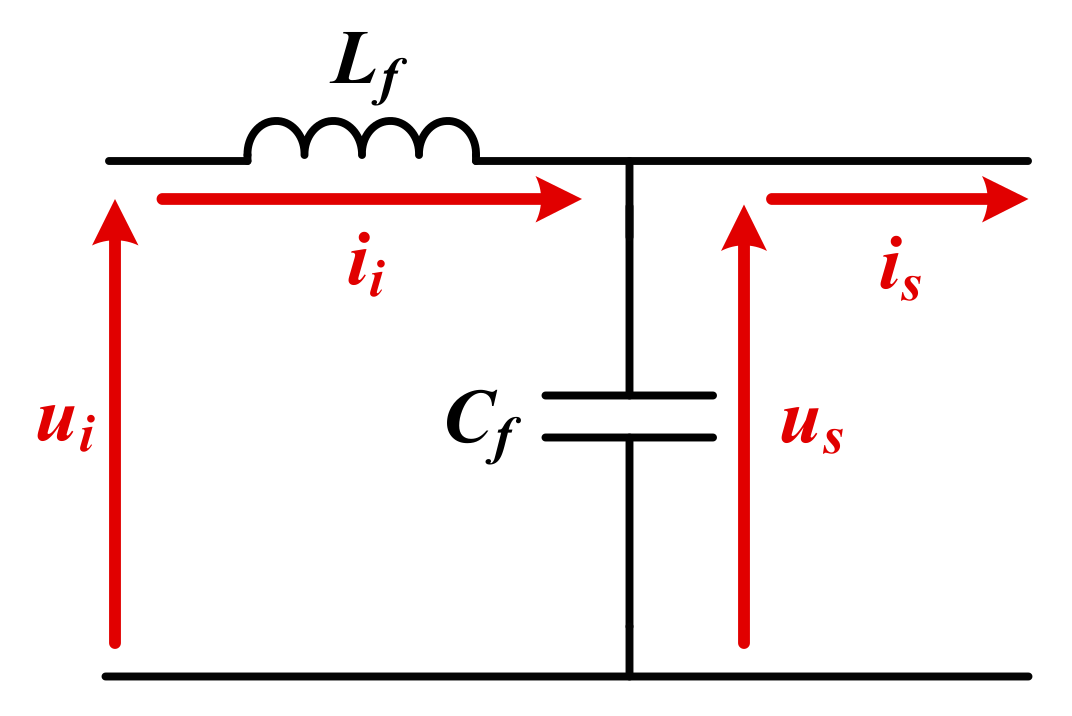
The schematic diagram of the LC filter (single phase) is depicted in
Figure 3.
The model of the LC filter is expressed as
where
usa,
usb and
usc are the phase voltages of the PMSM,
isa,
isb and
isc are the stator currents;
uia,
uib and
uic are the filter voltages,
iia,
iib and
iic are the filter currents;
Lf and
Cf are the inductance and capacitance of the filter, respectively.
By Clark transform, the model of the LC filter described in the stationary reference frame is given as
where
uiα,
uiβ are the filter voltages in the stationary reference frame, and
iiα,
iiβ are the filter currents.
It is assumed that the filter inductance and capacitance are three-phase symmetric. Furthermore, the resistance and mutual inductance are very small in practical applications, so that they can be neglected [
4,
5]. Hence the center-point voltage of the filter is equal to that of the motor. Therefore, the mathematical model of the PMSM drive system with LC filter in the stationary reference frame is given by Equations (1) and (2) and Equations (9)–(12).
2.2.2. Switching Function Model
The sum of three phase voltages is expressed as
The voltage from the neutral point n to the ground is defined as uing, and the voltages from the phases to the ground are defined as uiag, uibg and uicg, then it can be obtained that
By the sum of Equations (14)–(16), it can be derived that
Substituting Equation (17) into Equations (14)–(16), it is obtained that
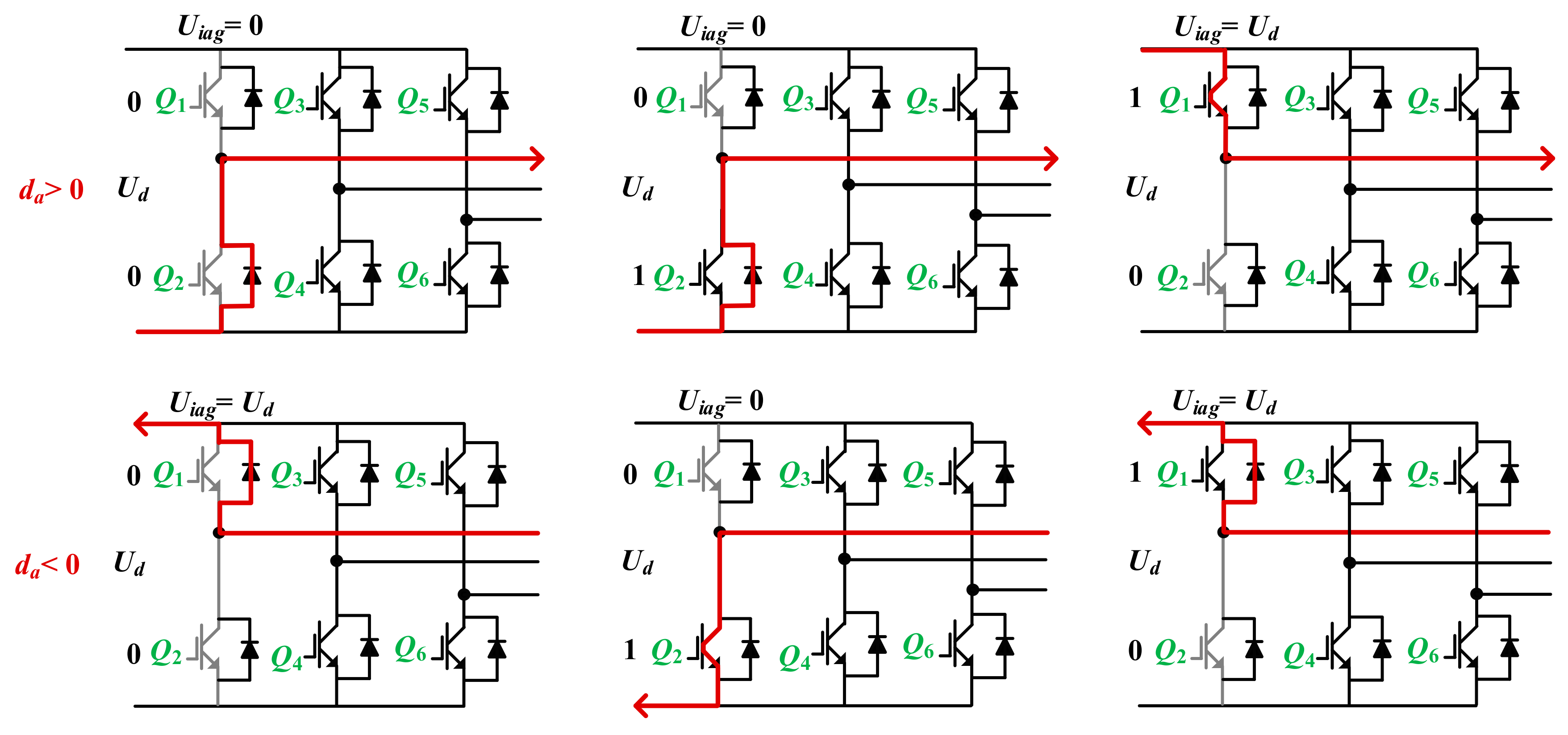
The filter voltage of phase A is determined by the on-off states of
Q1/
Q2 and the current directions.
Figure 4 shows the filter voltages of phase A in different on-off states and current directions under the healthy case. In
Figure 4, “1” represents that the switch is on, and “0” represents that the switch is off. The variable
da represents the direction of the current.
Ud represents the DC-link voltage. Similarly, filter voltages of the other two phases can also be concluded. There are six possible combinations between the on-off states and current directions. Filter voltages under different combinations of on-off states and current directions are illustrated in
Table 1.
s1/3/5 and
s2/4/6 represent the on-off states of the switches
Q1/
Q3/
Q5 and
Q2/
Q4/
Q6, respectively.
The switching function is defined by the on-off states of the power switch
s, the direction of the filter current
d, and the DC-link voltage
Ud. The value of the function is 1 or 0. The phase-to-ground voltages of the filter
uiag,
uibg and
uicg can be given by the switching functions. From
Table 1, the phase-to-ground voltages
uiag,
uibg and
uicg are expressed as
sa, sb and sc are defined for mathematical simplification. Substituting Equations (21)–(23) separately into Equations (18)–(20), the filter voltages uiag, uibg and uicg expressed by the switching functions are obtained by
By Clark transform, the switching function model (24)–(26) can be transformed into the equations about the filter voltages in the stationary reference frame
uiα and
uiβ:
2.3. Sliding Model Observer
In this study, the sliding mode observer is chosen. The sliding mode observer is effective, and robust to the variation of parameters. In the proposed diagnostic technique, there are no extra current/voltage sensors. The estimated filter voltages and other state variables are obtained by the proposed SMO. In this study, the novelty is that this SMO considers the model of the LC filter. The SMO is analyzed in this section.
2.3.1. Observer Description
The system model considering the LC filter in the stationary reference frame is described by Equations (1) and (2) and Equations (9)–(12). According to the model, the state equations used for the SMO can be written as [
33]
where
x is the state variable vector,
u is the input variable vector, and
A,
B,
C are system matrices.
In this paper, the state variables are chosen as
The vector of output variables
y is
The vector of input variables
u is
The filter voltages
uiα and
uiβ are regarded as the disturbances, so the initial values of their derivatives in the observer can be set to 0 [
34]. Hence, the system matrix
A used by the observer is given as
Moreover, the system matrices
B and
C are
The SMO is obtained according to state equations. The SMO is defined as
where ˆ denotes the estimated variable, the function sgn(·) denotes the signum function, and
G is the gain matrix. The robustness and dynamic performance of the observer are determined by
G. In the SMO, the back electromagnet forces
esα and
esβ of the motor in the observer are calculated by Reference [
34]
where
ψf is the flux linkage,
ωe is the electrical speed of the rotor, and
θe is the electrical position of the rotor; the subscript
α and
β represent the
α axis and
β axis in the stationary reference frame, respectively.
The schematic diagram of the SMO is illustrated in
Figure 5. The estimated and output variables are estimated by the SMO. The differences between the outputs of the plant and the observer are fed back into the SMO.
2.3.2. Design of Gain Matrix
In the literature, SMOs are always designed by Lyapunov’s method. In this study, the Lyapunov’s method is not used, because the observer is much more complicated, due to the LC filter. The Lyapunov’s function may also be complicated. Therefore, the method based on state transformations is used to design the gain G in this study.
To design the gain
G, the matrices
x,
y and the system matrices
A,
B,
C are divided into sub-systems [
33]:
The gain G can also be divided into two sub-matrices.
Hence, the SMO is rewritten by two subsystems [
33]:
The errors are expressed as
Consequently, if the sub-matrix
G1 could be selected large enough,
can be ensured in theory. Therefore, it can be obtained that
It should be noticed that ensuring the assumption is difficult in practical cases. In the observer, can be seen as a feedback, and the matrix G1 can be seen as a control parameter. is difficult to be 0, but it can maintain a relatively small value by the regulation. In practical cases, that is acceptable because any closed-loop observer has definite stability.
It can be seen that the errors in Equation (35) tends to be 0 only by the real parts of all the eigenvalues of the term
A11-
G2A21 being less than 0. All the eigenvalues of the matrix must have negative real parts to ensure the observer being stable and converging to actual values. Besides, if the observer poles are located closer to the imaginary axis, the observer tends to be more stable. However, it will have a slower dynamic response. If the observer poles are designed too far away from the imaginary axis, it will be more responsive, but less stable because of the influence of measurement noise. The term
A11-
G2A21 has six eigenvalues, but the equations in
α and
β axis are symmetrical. Therefore, the pole-placement problem for a 6×2 matrix is transformed into a pole-placement problem for a 3×1 matrix
G2′. If the poles of
G2′ are selected as
μ1,
μ2 and
μ3, the desired characteristic polynomial is as follows
The matrix
G2′ is calculated by Ackermann’s formula [
35]
where
P0 = [
A21 A21A11 A21A112]
T.
2.4. Analysis of Fault Signatures
In theory, when the drive system is in a healthy case, the expected filter voltages are equal to the actual ones, so the residual errors are always 0 [
18,
21]. If the open-switch faults occur, residual errors may not be 0 anymore. In this section, different theoretical residual errors under different faulty locations are analyzed.
2.4.1. Fault Signatures of Phase A
As shown in
Figure 2, the on-off states of the six power switches
s1~s
6 are calculated by the SVPWM module. The digital signals
s1~
s6 are amplified and used to drive the six power switches
Q1~
Q6. Therefore, the voltages of the three phases
uiA,
uiB and
uiC can be generated by the turn-on and turn-off of the power switches.
If the open-switch fault occurs on the power switch
Q1, the expected value
s1 is still determined by the space-vector PWM (SVPWM) algorithm, while the actual switching variable
s1f is 0. According to Equations (21)–(23) and Equations (27) and (28), the actual filter voltages in the stationary reference frame can be expressed as
where
uiαf1 and
uiβf1 are the actual filter voltages in the stationary reference frame when the open-switch fault occurs on
Q1. By Equations (38) and (39), it can be seen that the residual error in the
α axis is changed due to the fault. The residual errors are given as
where
rα and
rβ are the residual errors.
rα varies in the positive axis when there is an open-switch fault on
Q1.
Similar to the previous case, if the open-switch fault occurs on
Q2, the actual switching variable
s2f is 0, and the expected variable
s2 is still determined by the SVPWM module. Thus, the actual filter voltages in the stationary reference frame are expressed as
where
uiαf2 and
uiβf2 are the actual filter voltages in the stationary reference frame when the open-switch fault occurs on
Q2. Hence, the residual errors can be given as
It can be seen that rα changes in the negative axis when the fault occurs on Q2.
2.4.2. Fault Signatures of Phase B
If the open-switch fault occurs on
Q3, the actual switching variable
s3f becomes 0, but the expected variable
s3 is determined by the SVPWM module. The residual errors between the expected and actual filter voltages are given as
If the open-switch fault occurs on
Q4, the voltages in the stationary reference frame are expressed as
2.4.3. Fault Signatures of Phase C
Similar to previous cases, when the open-switch fault occurs on Q5, the actual switching variable s5f is 0, but the expected variable s5 still varies. The residual errors are expressed as
When the open-switch fault occurs on
Q6, the residual errors are expressed as
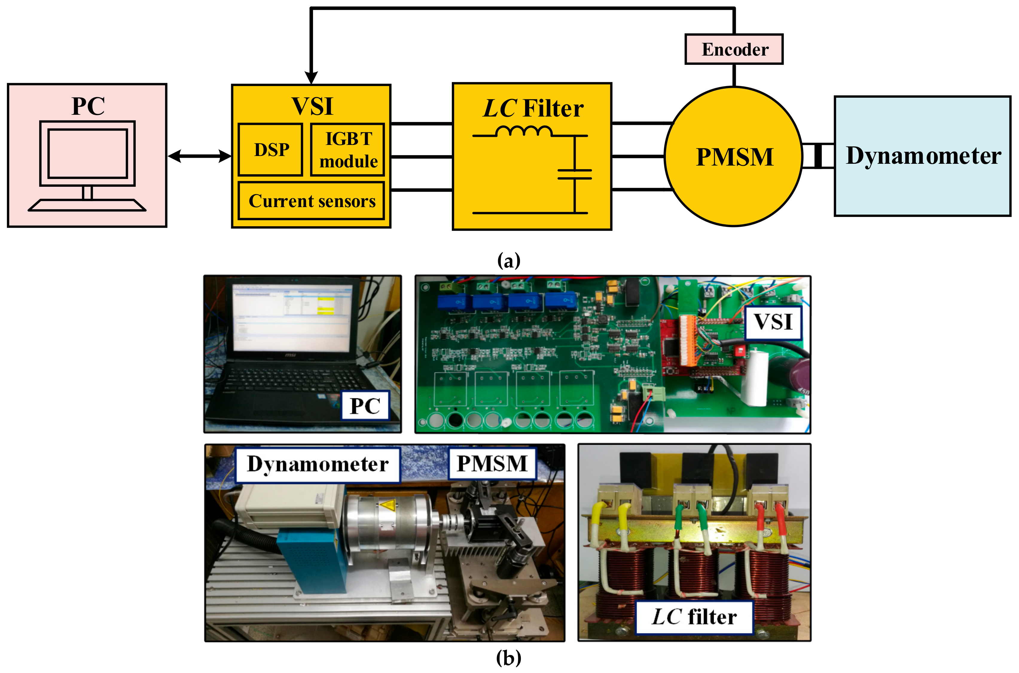
2.5. Experimental Setup
The proposed techniques were tested on a 750-W PMSM drive system. The block diagram of the experimental setup is shown in
Figure 6a, and the photograph is shown in
Figure 6b. The LC filter was equipped between the inverter and PMSM. The load torque was produced by the dynamometer (Dongguan Tension Technology Co., Ltd). The encoder measured the rotor position. The filter currents
iia and
iib were measured by the current sensors CASR-6 (LEM Electronics Co., Ltd.) on the inverter board. The filter currents
iiα and
iiβ were measured and transferred to the digital signal processor (DSP) TMS320F28069M (Texas Instruments Co., Ltd.). The model of the power switch module was FS30R06W1E3 (Infineon Technologies Co., Ltd.). The power switches were driven by the chips 1ED020I12-FT (Infineon Technologies Co., Ltd.). The open-switch fault was realized by the turn-off of the power switch.
The parameters of the PMSM and LC filter are given as follows: The flux linkage is 0.06 Wb; the stator resistance is 0.72 Ω; the stator inductance is 0.0041 H; the rated current is 4.06 A; the rated load is 2.3 N·m; the number of poles are 10; the filter inductance is 0.0004 H; the filter capacitance is 0.00003 F.
The DSP was utilized as the digital control unit to implement all the algorithms (PI controllers, SVPWM, SMO, proposed fault diagnostic process). The PWM switching frequency was 16,000 Hz, which equals to the sampling frequency. The process of the software program was:
The rotor speed ωe was calculated by the measured rotor position;
The currents iia and iib were transformed to the currents in the stationary reference frame iiα and iiβ;
PI regulators and SVPWM module ran, thus calculating the voltage references uiα* and uiβ*;
The fault diagnosis method which started from the switching function model ran;
The SMO ran to calculate the estimated voltages and with other state variables;
The residual errors rα and rβ were calculated;
If the fault was detected, the fault signal outputted, and the fault location was detected by rα and rβ;
The flowchart of the proposed method is shown in
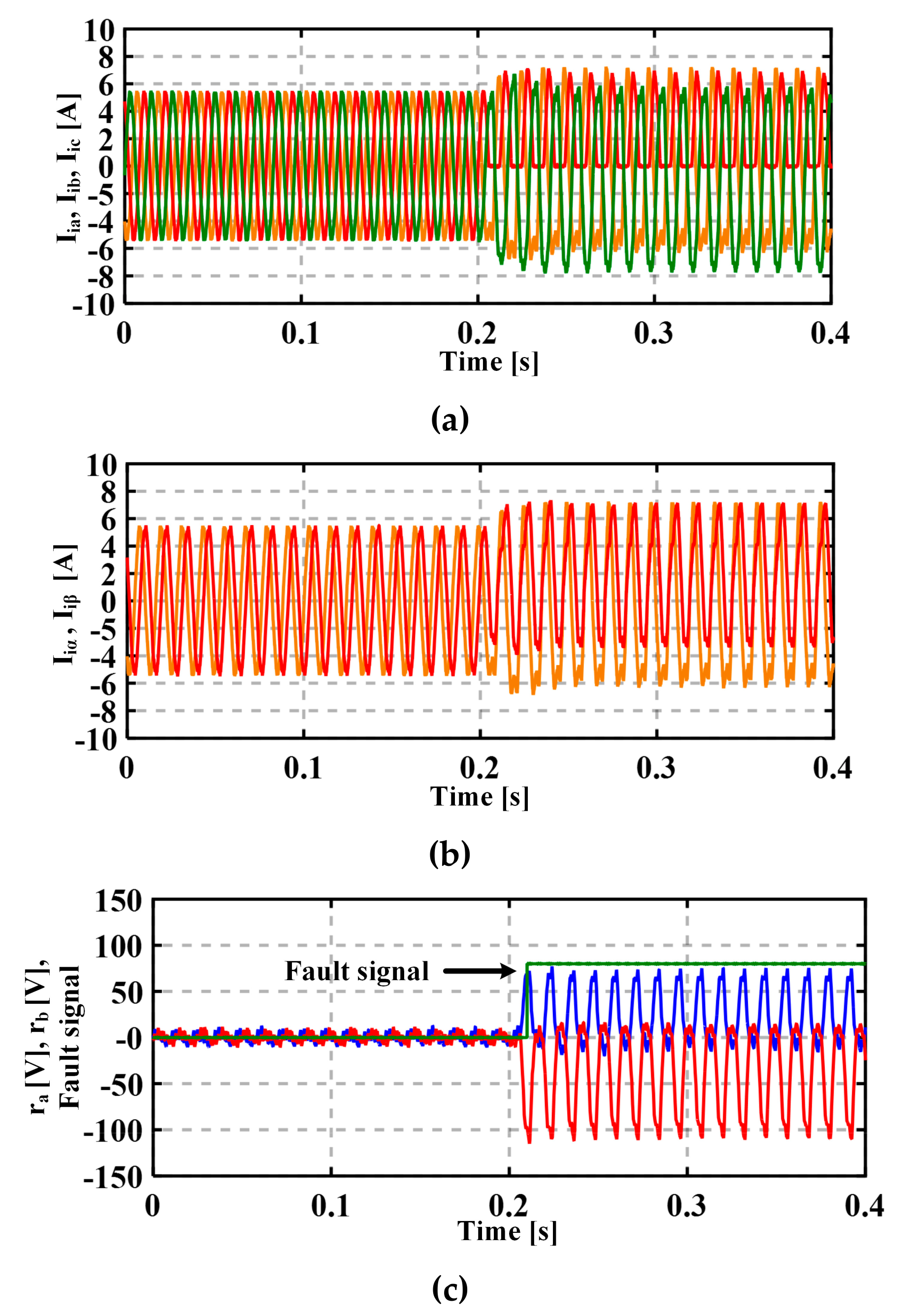
Figure 7. In practical applications, there must be errors between the actual and estimated values. Consequently, in order to implement the proposed method in practical applications, the threshold of the residual error in the software program should not be a value 0, but an interval. When the residual error is in the selected interval, the power switches are considered as in a healthy case. The threshold interval is set to (−9, 9).
3. Results
The system was tested under the rated load (2.3 N·m) in the experimental tests.
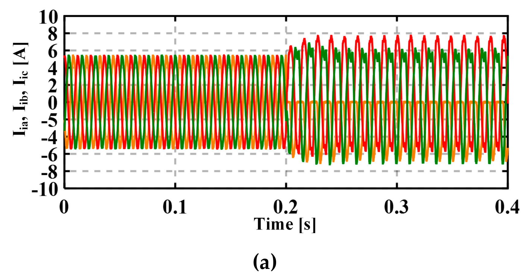
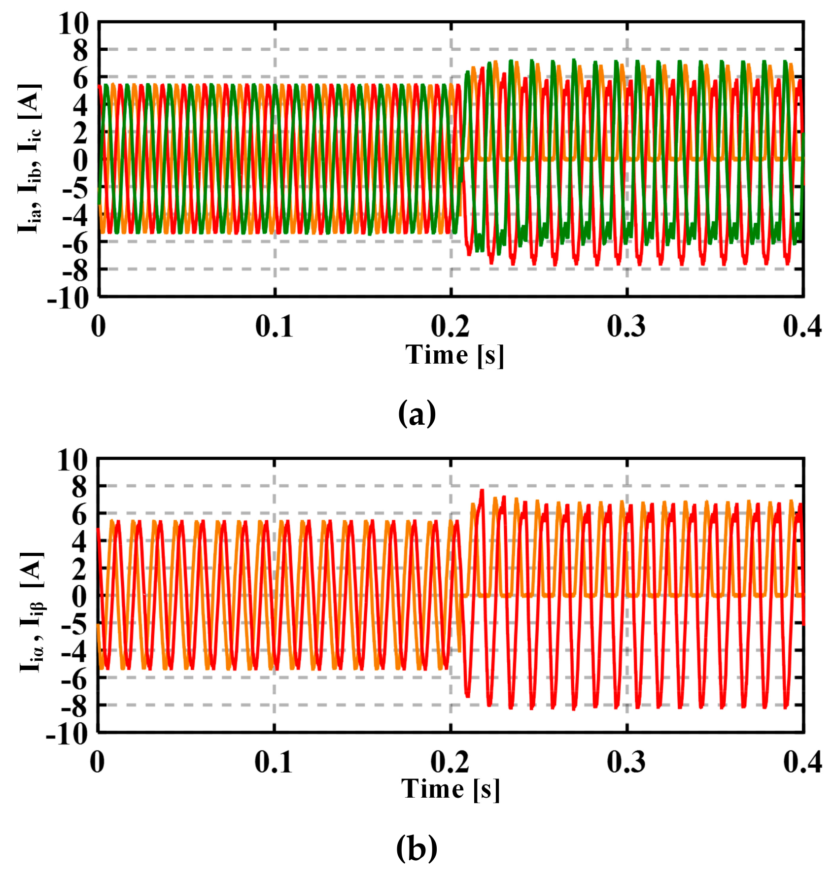
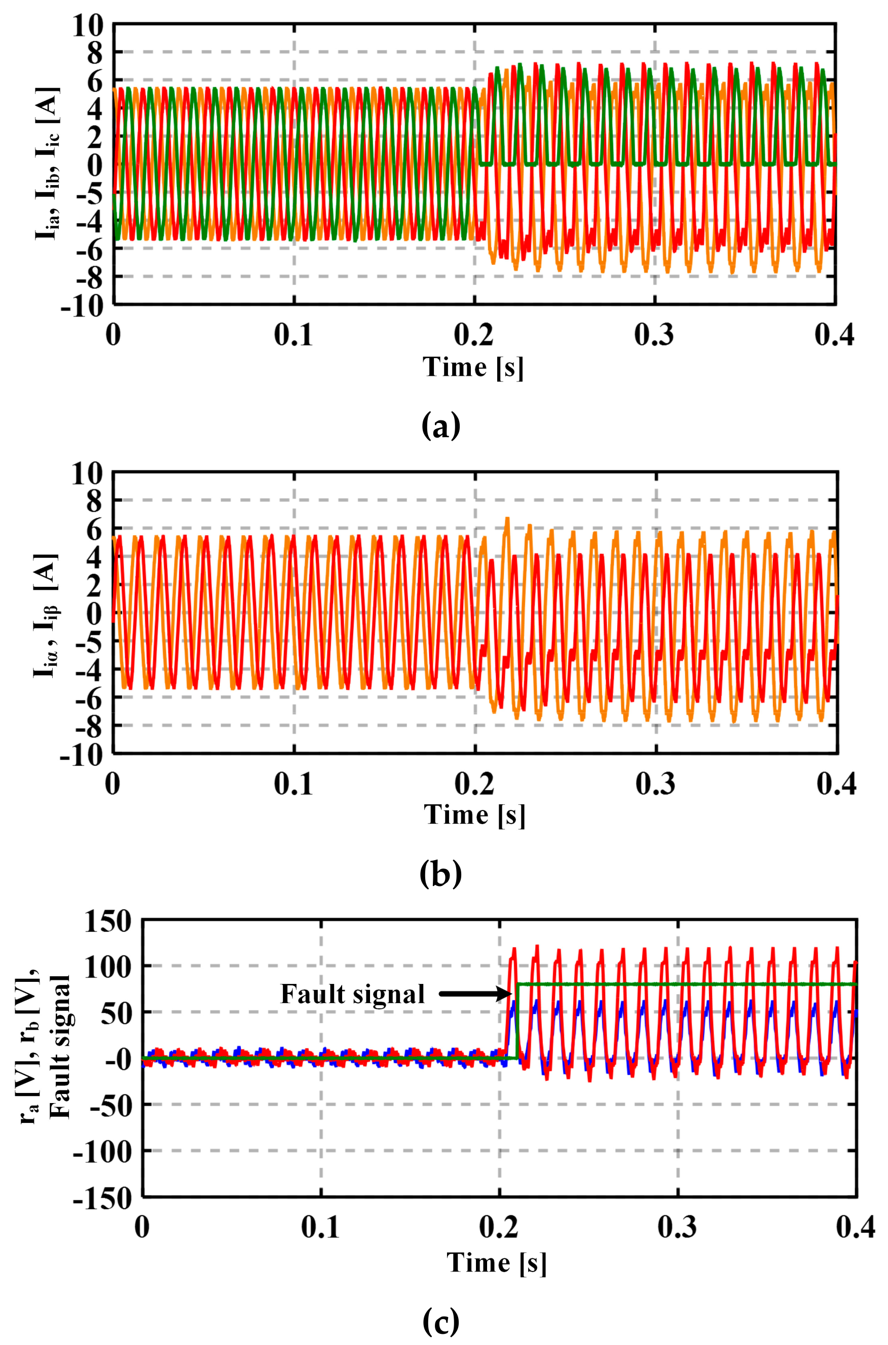
Figure 8 shows the experimental results when the open-switch fault occurs on
Q1.
Figure 8a shows the filter currents of the three phases
Iia (yellow),
Iib (red) and
Iic (green).
Figure 8b shows the filter currents in the stationary reference frame
iiα (yellow) and
iiβ (red).
Figure 8c shows the residual errors
rα (blue) and
rβ (red), and the fault signal. The PMSM is in a healthy case before 0.2 s. After the power switch
Q1 is open-circuit at 0.2 s, the filter current of phase A
iia cannot flow through the power switch
Q1. As shown in
Figure 1, the power switch
Q1 controls the positive part of the filter current of phase A
iia, so the filter current of phase A
iia becomes unidirectional and asymmetric from 0.2 s. The calculated currents in the stationary reference frame
iiα and
iiβ are not symmetrical any more. Before the open-switch fault on the power switch
Q1 occurs, the residual errors
rα and
rβ are both in the selected interval (−9, 9). After the fault occurs, the residual error
rα is not in the threshold interval any more, but varies in the positive axis. The other residual error
rβ is still in the interval. Hence, the fault signal of the power switch
Q1 can be acquired according to Equations (39) and (40).
Figure 9 shows the experimental results when the open-switch fault occurs on
Q2.
Figure 9a shows the filter currents of the three phases
Iia (yellow),
Iib (red) and
Iic (green).
Figure 9b shows the filter currents in the stationary reference frame
iiα (yellow) and
iiβ (red).
Figure 9c shows the residual errors
rα (blue) and
rβ (red), and the fault signal. The PMSM is in a healthy case before 0.2 s. After the power switch
Q2 is open-circuit at 0.2 s, the filter current of phase A
iia cannot flow through the power switch
Q2. The power switch
Q2 controls the negative part of the filter current of phase A
iia, so the filter current of phase A
iia only has the negative part from 0.2 s. Hence, the calculated currents in the stationary reference frame
iiα and
iiβ are not symmetrical any more. After the fault occurs, the residual error
rα varies in the negative axis, while the residual error
rβ is still in the selected interval. Therefore, the fault signal of the power switch
Q2 can be acquired according to Equations (41) and (42).
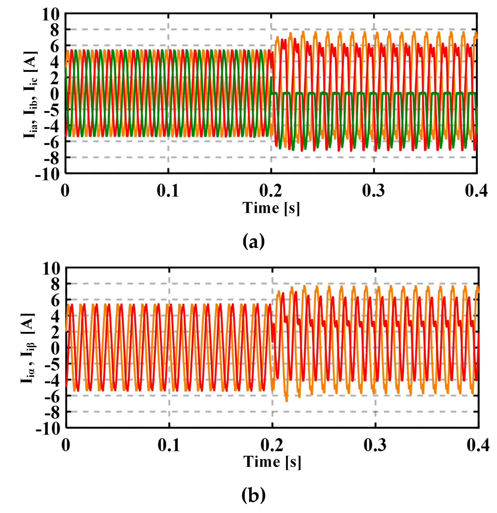
Figure 10 shows the experimental results when the open-switch fault occurs on
Q3 at 0.2 s.
Figure 10a shows the filter currents of the three phases
Iia (yellow),
Iib (red) and
Iic (green).
Figure 10b shows the filter currents in the stationary reference frame
iiα (yellow) and
iiβ (red).
Figure 10c shows the residual errors
rα (blue) and
rβ (red), and the fault signal. After the power switch
Q3 is open-circuit at 0.2 s, the filter current of phase B
iib cannot flow through the power switch
Q3. The power switch
Q3 controls the positive part of the filter current of phase B
iib, so the filter current of phase B
iib only has the negative part from 0.2 s. After the fault occurs, the residual error
rα varies in the negative axis, while the residual error
rβ varies in the positive axis. Therefore, according to Equations (43) and (44), the fault signal of the power switch
Q3 can be acquired.
Similarly,
Figure 11,
Figure 12 and
Figure 13 show the experimental results when the open-switch faults occur on
Q4,
Q5 and
Q6, respectively.
Figure 11a,
Figure 12a and
Figure 13a show the currents of the three phases
Iia (yellow),
Iib (red) and
Iic (green).
Figure 11b,
Figure 12b and
Figure 13b show the currents in the stationary reference frame
iiα (yellow) and
iiβ (red).
Figure 11c,
Figure 12c and
Figure 13c show the residual errors
rα (blue) and
rβ (red), and the fault signals. After the faults occur, the residual errors
rα or
rβ changes. Different waves of residual errors can indicate different faulty locations.
4. Discussion
This paper proposes a novel SMO-based open-switch diagnostic method for permanent-magnet synchronous motor drive connected with LC filter. The expected filter voltages are acquired by the switching function model, and the filter voltages are estimated by the SMO. Besides, other estimated state variables are used for the closed-loop control of the drive system. The fault signals are obtained by the residual errors, thus open-switch faults being detected and located.
By implementing the proposed method, the main finding is that the proposed method can detect the faults effectively, and open-switch fault in each power device can be located quickly. The proposed technique can be used for other PMSM drive connected with LC filter at any power level. Compared with other observer-based open-switch fault diagnostic methods, the other methods cannot detect the faults when LC filter is connected. By considering the mathematical model, the proposed technique can detect and locate the open-switch faults for the PMSM drive system connected with LC filters. Because the proposed diagnostic method is based on the voltages, it can be utilized in both open- and closed-loop control systems. The overall diagnostic procedure is not difficult to implement, and extra sensors are not necessary.
The limitation of this study is that the proposed technique cannot detect and locate the faults if the faults occur on two or more power switches simultaneously. In future studies, fault diagnosis for two or more switches and fault tolerance control methods will be researched.
When the proposed method is applied in practical cases, the most important parts are the SMO and the threshold interval. The gain matrix of the SMO should be designed to keep the stability and quick response. The threshold interval should be selected appropriately to avoid false alarms. The gain matrix can be designed by a particular criterion, as analyzed before. However, the interval is difficult to design by any theoretic criterion. The interval can be selected by trial and error. Furthermore, in the SMO, the sliding surface is a signum function which may lead to the chattering. For suppressing the chattering, the sliding surface can also be a saturation function or sigmoid function.


