Thermophysical Properties Estimation in Annealing Process Using the Iterative Dynamic Programming Method and Gradient Method

Abstract

In annealing, steel coils should be heated and consequently cooled according to the technological prescription defined for the annealed type of steel. It is appropriate to develop the systems and methods for estimation of the steel coil inner temperature for that reason. The proposal for such a system of indirect measurement of inner temperature is described in this study. This system, in the form of the mathematical model, is developed based on the theory of heat transfer and needs thermophysical parameters as inputs. In many cases, the thermophysical properties are difficult to access or unknown for the specific composition of the material being processed. In this paper, two optimization methods were applied to estimate two thermophysical properties. The application of the iterative dynamic programming method is aimed to estimate optimal thermal diffusivity. The verification of this method was performed on 11 laboratory measurements. The algorithm of the gradient method was used for estimating thermal conductivity and was verified on seven operational measurements. Results show that the optimized values of thermophysical properties increased the accuracy of the steel coil inner temperature estimation in the locations nearer to the steal coil central axis.

1. Introduction

In the production of steel sheets, the steel is cold rolled into sheets and then coiled into coils, which are supplied to customers. The subsequent annealing process is a method of heat treatment of alloys. This process aims to change the mechanical properties of the material by changing its microscopic structure at a high temperature (i.e., according to the technological prescription) because the cold rolling process makes the steel hard, brittle, and difficult for further processing. The coils are heated to the desired temperature, maintained at this temperature until the coldest place of the coil reaches this temperature, and then the coils are cooled in the annealing process. This entire process is called the annealing regime. The temperature of annealing is often near to melting temperature, but it cannot be higher. The aim of the heating is often to increase toughness, ductility, and tensile strength. Heating is often used in connection with the steel and cast iron, but it is possible to use it for other alloys as well.

This process modeling (i.e., the prediction of the heating, the maintaining, and the cooling time) is a very hard and difficult task. The indirect measurement system (e.g., in the form of two-dimensional thermal models described in [1]) can be used to solve this task (i.e., for the prediction of the coil temperature behavior). Indirect measurement system described in this paper enables one to determine temperatures in annealed coil based on the atmosphere temperature that is directly measured. For creating systems of indirect measurement, the dependencies of thermophysical parameters (e.g., thermal conductivity, thermal diffusivity, specific heat capacity, density, the emissivity of the particular materials in which the temperature is to be measured, respectively heat flow) are required. It is very important to determine the thermal conductivity or thermal diffusivity for anisotropic materials (batch), which is typical for the coil that is annealed. Table values of these thermal parameters are not available for all materials for different reasons (e.g., research of new material). Research on these parameters is needed through other means (e.g., utilization optimization methods). A novel method of indirect measurement based on neural networks was published in [2].

The aim of this paper is the proposal of optimization methods for determining thermophysical properties that are applied to the increase of accuracy for the system of indirect temperature measurement (SIMT) in the annealing process. The SIMT has the form mathematical model, which is the extension of the models described in [1,3]. The task of this system is the calculation of inner temperatures based on measuring an annealing atmosphere temperature. The annealing atmosphere temperature is directly measured between the protection bell and annealed coils.

2. Overview of Thermal Properties Research

Each heat treatment includes heating a metal or alloy at the prescribed temperature, holding this temperature, and cooling to reach the prescribed changes in the microstructure and mechanical properties. Basic variables in the technology of heat treatment are time and temperature (i.e., change of temperature depended on time), that means the speed of heating or cooling. State diagrams are the basis for studying of possibilities of a material’s heat treatment. They characterize the material in equilibrium, show what temperature and concentrate conditions are needed to phase transformations, and how the solubility of items changes in dependence on temperature.

The microstructure evolution of low carbon cold-rolled medium manganese steel was studied in [4]. The impact of a different reverse-phase transformation annealing temperature was used for this purpose. The results showed that austenite volume change occurred, the tensile strength increased, and the yield strength declined at the increment of the annealing temperature. The effect of the deformation temperature on the deformation mechanism and tensile properties of the chosen steel was described in [5]. It was found that the dislocation glide gradually became the main deformation mechanism with the increase of the deformation temperature. The change of the microstructure and mechanical properties by the impact of welding heat input was examined in [6]. The results of this paper showed that with the increase of heat input, the tensile strength of the samples which contained the weld and heat affected zones was increased.

The heat treatment influences the steel thermophysical properties besides the resulting steel microstructure. The materials thermal properties at high temperatures are not always readily available but have importance in the industrial production and the theoretical simulation area. The paper [7] described a technique to get the temperature dependence of the thermal conductivity and the specific heat by using only one experiment. The finite element method and the pattern search method was used for optimizing the thermal properties in this paper.

Various approaches in determining thermophysical properties have been developed in the world. The authors in paper [8] describe the method for determining the thermal conductivity of the insulation material. This non-contact method solves the nonlinear problem of the relationship between thermal conductivity and frequency change by neural networks. This method was verified by experiment and the least squares method. The thermal conductivity prediction model of the rocks was described in [9]. The adaptive network-based fuzzy inference system (ANFIS) and multivariate regression analysis was used to determine the thermal conductivity of the materials used for building construction.

The estimation of the effective thermal conductivity for the silicate materials is described in [10]. Based on the measurement of experimental data, the thermal conductivity of silicate matrix was determined. The thermal conductivity of this silicate matrix is calculated by the extrapolation of the effective thermal conductivity vs. the porosity functions to the zero porosity. Rostami et al. in [11] described the development of a model capable of predicting dry sandstone thermal conductivity by implementing a machine algorithm of a least square support vector. Another study developed a method for determining composted material thermal conductivity by using the TP08 probe [12]. The significance of the influence to the results by the selection of a signal fragment at the determination of thermal conductivity was examined.

In recent times, IRT (i.e., infrared thermography) and photo-pyroelectric techniques have been applied for the measurement of solid samples’ thermal diffusivity. The tested material was the sample of a glassy carbon where these techniques were used to gain the thermal diffusivity of a sample. Experiments and numerical simulations were performed in order to evaluate the coupling fluid influence to the thermal diffusivity values by a photo-pyroelectric technique, assuming that the values of thermal diffusivity obtained by thermography were correct [13]. Another method that was applied for a material’s thermal diffusivity determination was based on the Markov-Chain Monte Carlo method (MCMC) [14].

The photoflash technique was used for measuring the gold nanofluids thermal diffusivity by adjusting the theoretical temperature signal to the measured experimental data [15]. This technique was examined at room temperature and low concentration of these nanofluids, which the samples being obtained by the pulse laser ablation method.

The numerical approach for determining the materials thermal diffusivity was presented in [16], where solved the inverse problem by the Levenberg–Marquardt method. The evaluation of the inverse thermal diffusivity method was used following materials of Agar water gel, glycerol, and Ottawa quartz sand.

Kim et al. proposed a method for determining the heat transfer coefficient by the optimization algorithm. Authors have used the SQP (i.e., sequential quadratic programming) as an optimization algorithm to get the temperature dependence of the heat transfer coefficient. The objective function is expressed as a minimization of the difference between the calculated temperature and experimental obtained temperature [17].

Huiping et al. in [18] used the finite element method (i.e., FEM) and the gold section method (i.e., the optimization method) for the analysis of the inverse of the heat condition’s quenching process. The proposed method calculates the surface heat transfer coefficient according to the temperature curve. This curve is obtained by the experiment during quenching process. The basic theorems of optimization and inverse problems were analyzed in the heat transfer area by [19]. There, the stochastic and deterministic minimization methods were analyzed and compared. This analysis and comparison were made in finite and infinite dimensional space.

Recently, Sadeghzadeh et al. proposed the “Delaware modified” method, which has two basic tasks. The first task is determining the heat transfer coefficients, and the second task is determining the shell-side pressure drop. The non-dominated sorting genetic algorithm (i.e., NSGA-II) was used for the optimization of the objective function to find the best solutions. The task of the objective function was maximizing the heat transfer rate and minimizing the total cost [20].

The sheet-forming processes of varying complexity were analyzed in [21]. They presented the application and optimization of a coupled finite element simulation to the entire forming process. The simulation of this process is based on a nonlinear gradient-based optimization method. They optimized single or multiple design objectives with set constraints in a form sheet-forming response [21].

The optimization problem of improving the strip flatness in a strip coiling process was solved by the efficient metaheuristic in [22]. It is based on the differential evolution and the hybridization of teaching–learning-based optimization. It was found that the proposed hybrid method, especially at a large-scale design problem was effective for process optimization.

This section has shown the importance of determining the thermophysical properties for different types of materials as the existing table values are not sufficient. Nowadays, methods of thermophysical properties estimation using optimization approaches are used by researchers.

3. Research Methodology

The proposed research methodology for estimating the thermal conductivity and thermal diffusivity in the annealing process includes the following steps:

• Realization of control measurement (i.e., annealing regime) for the chosen quality type of the annealed coil. (i.e., obtaining temperatures in individual locations of annealed coil and annealing atmosphere temperature);
• The thermophysical properties initial setting;
• Proposal of the indirect measurement system for estimating inner temperatures of the annealed coil;
• Proposal for the optimization methods for estimating thermophysical properties.

3.1. Experimental Measurements

Durdan et al. realized laboratory and operating measurements to improve the annealing process. Realized measurements were used for the development of SIMT and to determine of thermophysical properties applied in SIMT. Measuring chains and measuring points are described in the following subsections [1,23].

3.1.1. Laboratory Measurements

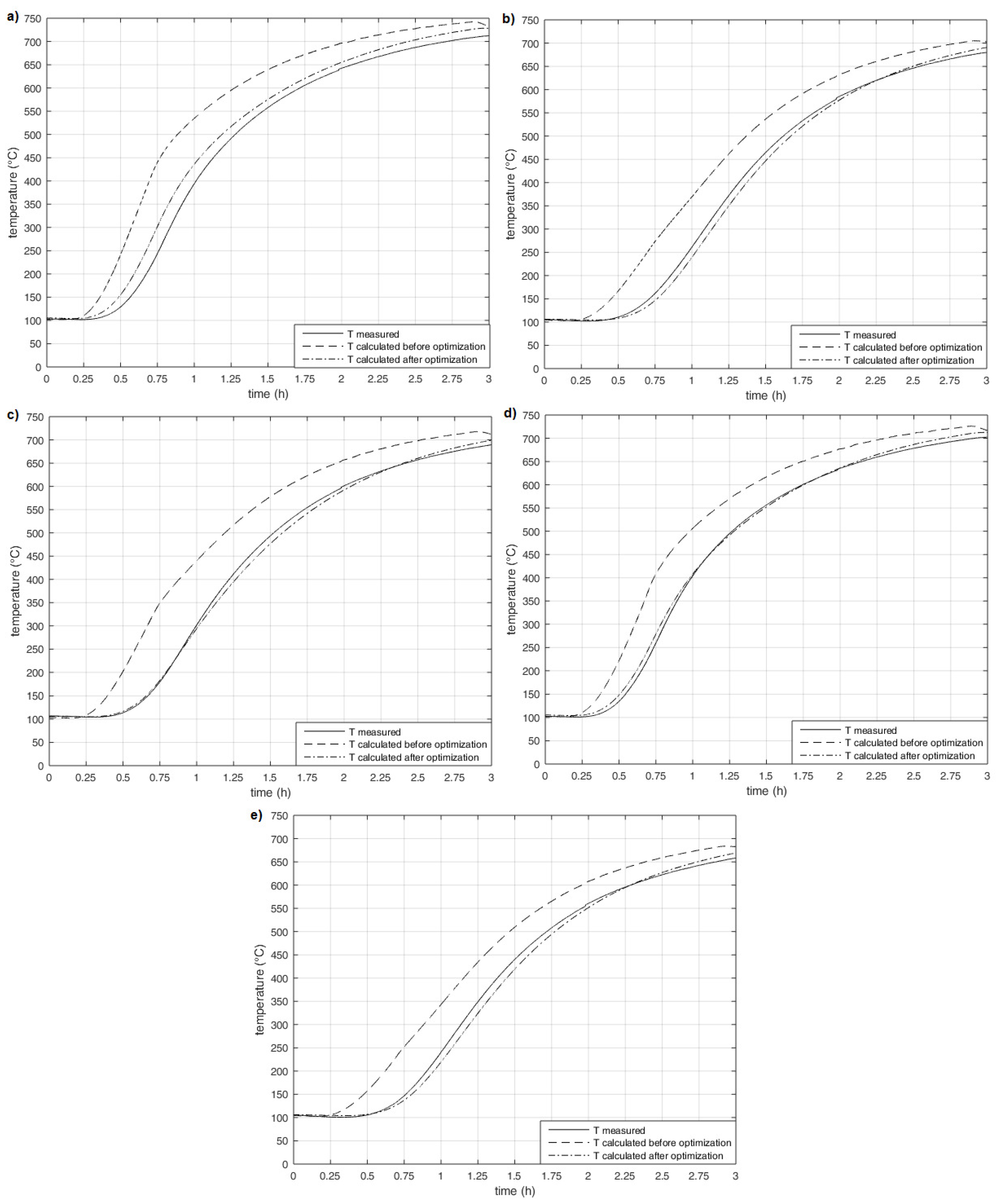
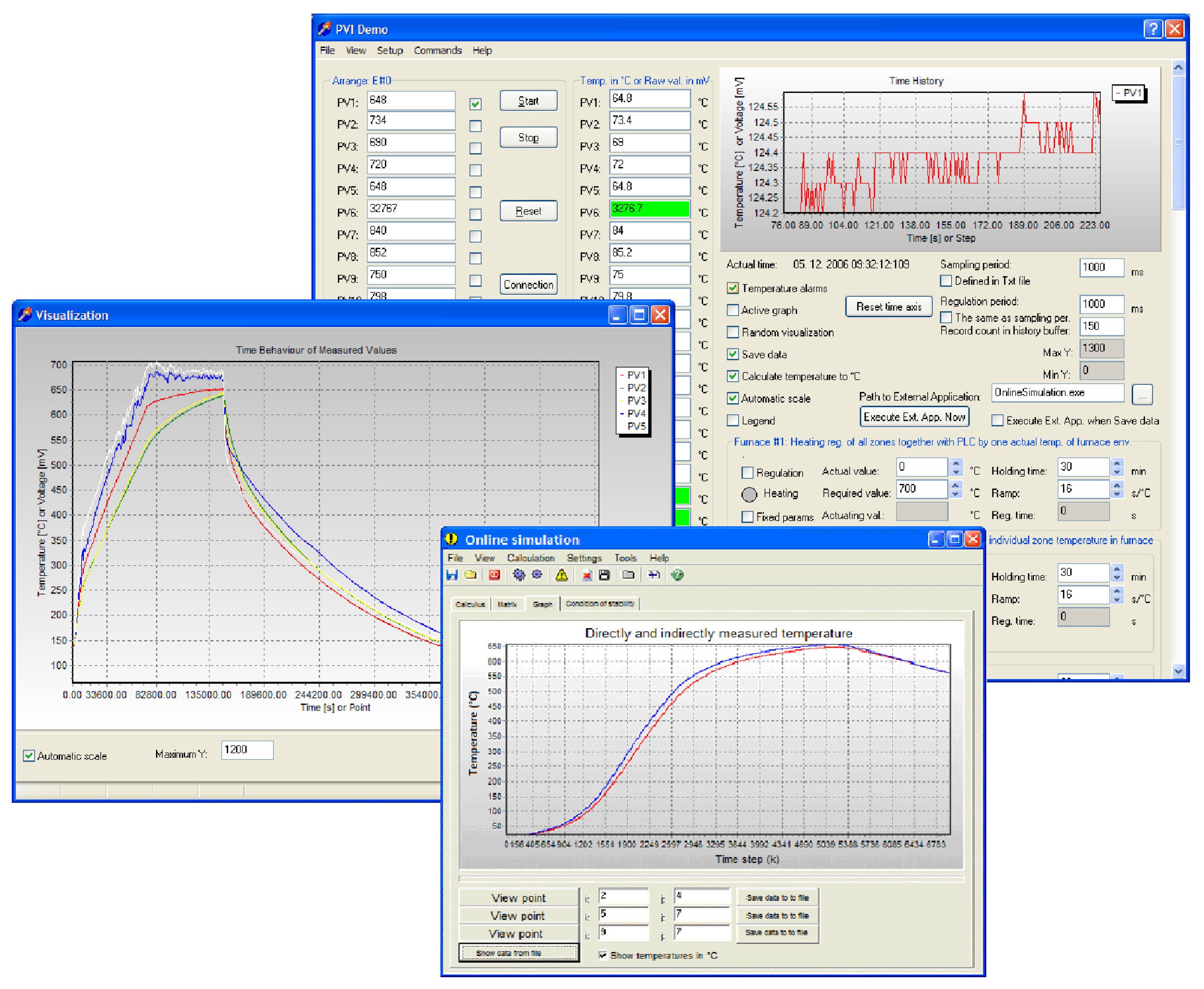
The laboratory measurements were performed on a laboratory bell furnace as it is described in [23]. A total of 11 measurements were performed in the laboratory furnace which were used for determining (i.e., with the utilization of the optimization method) the thermal diffusivity described in Section 3. The scheme of the measuring chain of realized measurements is shown in Figure 1. This Figure 1 shows the direct temperature measurement using the thermocouples of K type that are connected to the programmable logic controller (PLC). Monitoring and recording measured temperatures during the experimental annealing are performed on the connected computer. Data were transferred to the computer via the OPC protocol (Object Linking and Embedding for Process Control). The laboratory steel coil was created to the annealing process verification. A steel sheet with a thickness of 0.5 mm was used. 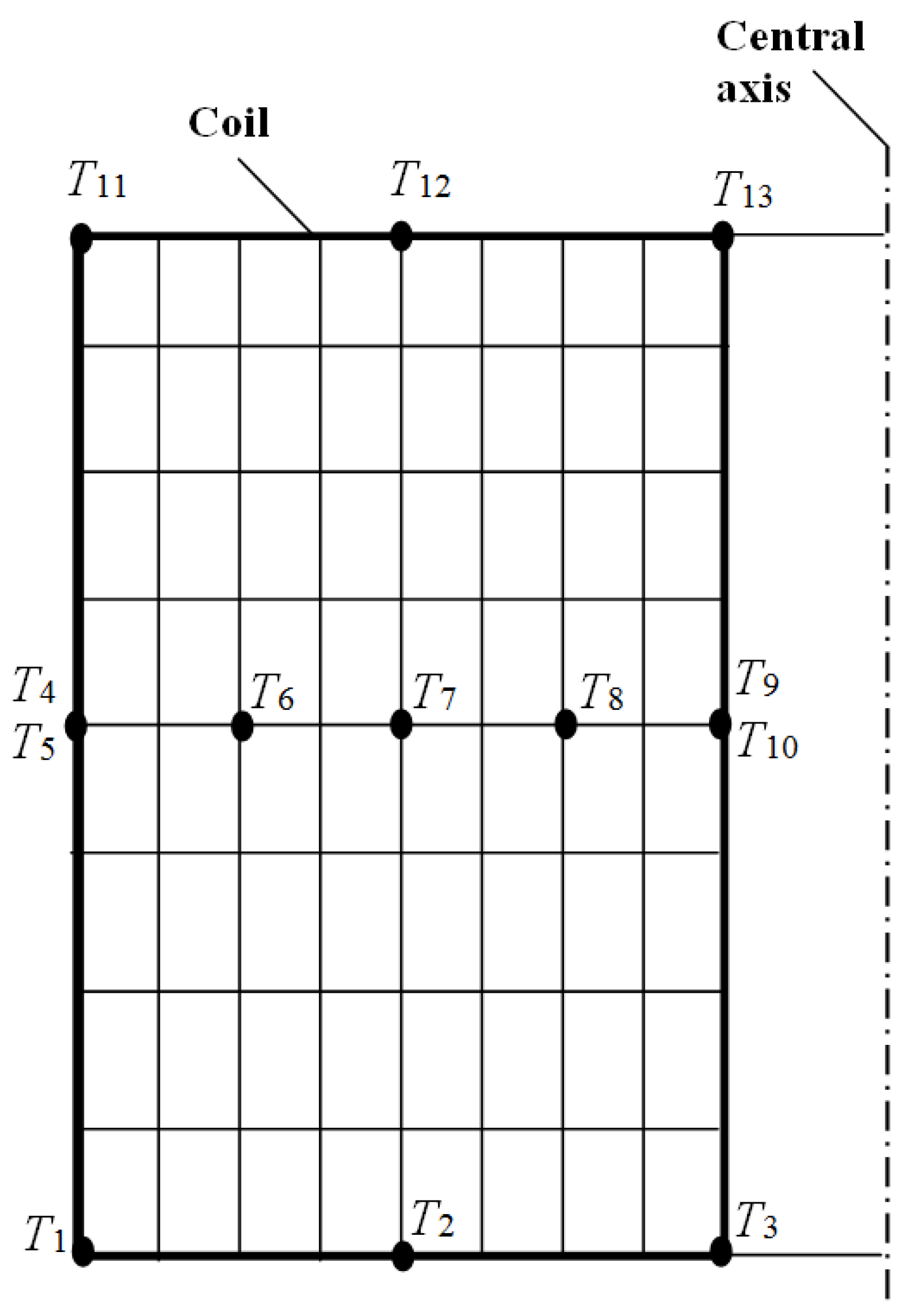The thermocouples of K type (i.e., marked $T_1$, $T_2$, ⋯, and $T_{17}$) were placed on the inside and on the surface of this coil. These thermocouples measured the coil’s inner and surface temperatures. The Figure 2 shows the measuring places of temperatures in the annealed coil sectional view. The positions of these measuring places correspond to dimensions of the two-dimensional network.

3.1.2. Operating Measurements

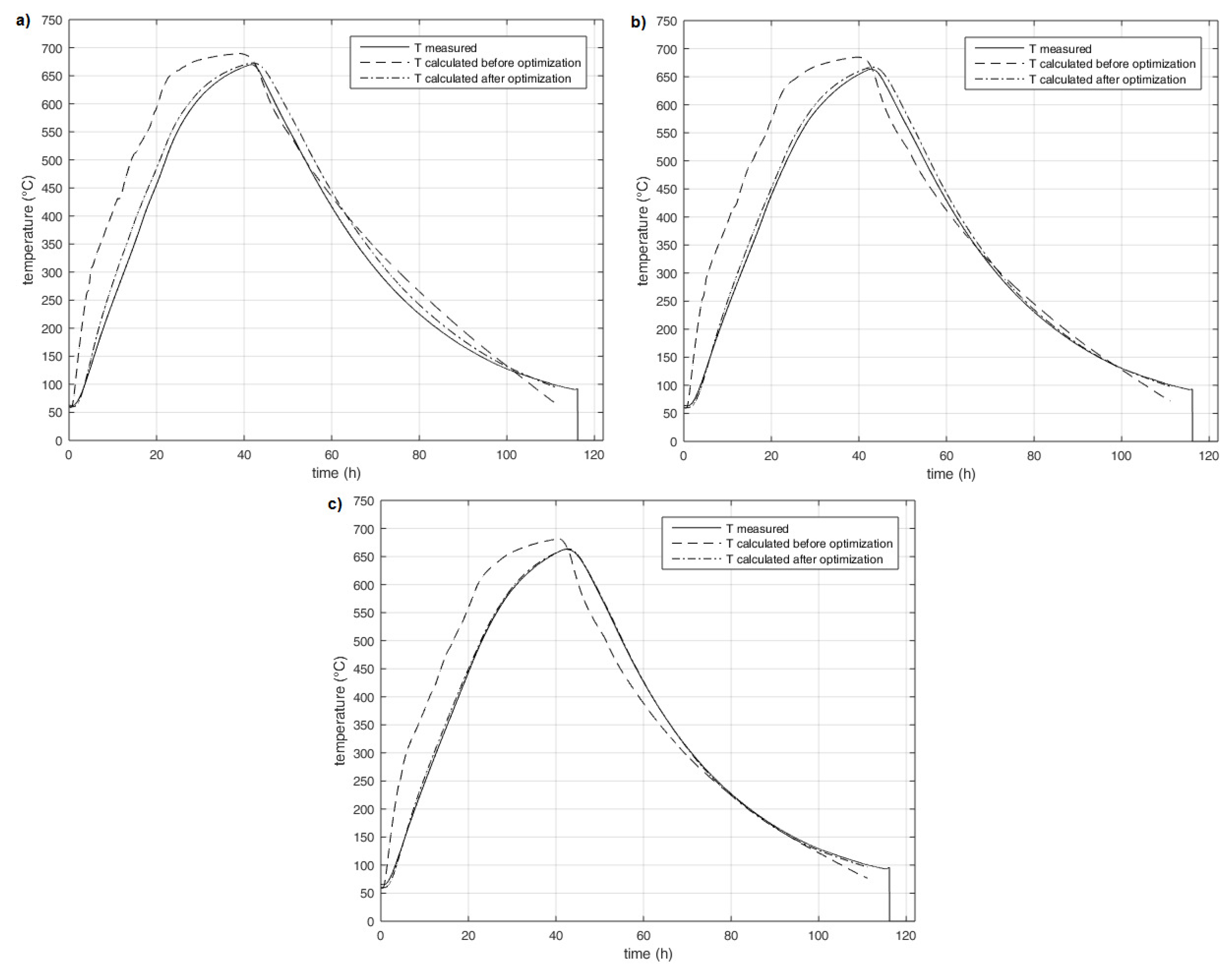
A total of 7 operating measurements were performed on the real bell furnace in an annealing plant [1]. The scheme of measurement chain for the realized measurements is shown in Figure 3. The temperature measurement were carried out on the same principle as in laboratory measurements. There were thermocouples of K type connected to the PLC and transfer of data from the PLC to the PC was ensured using the OPC protocol. 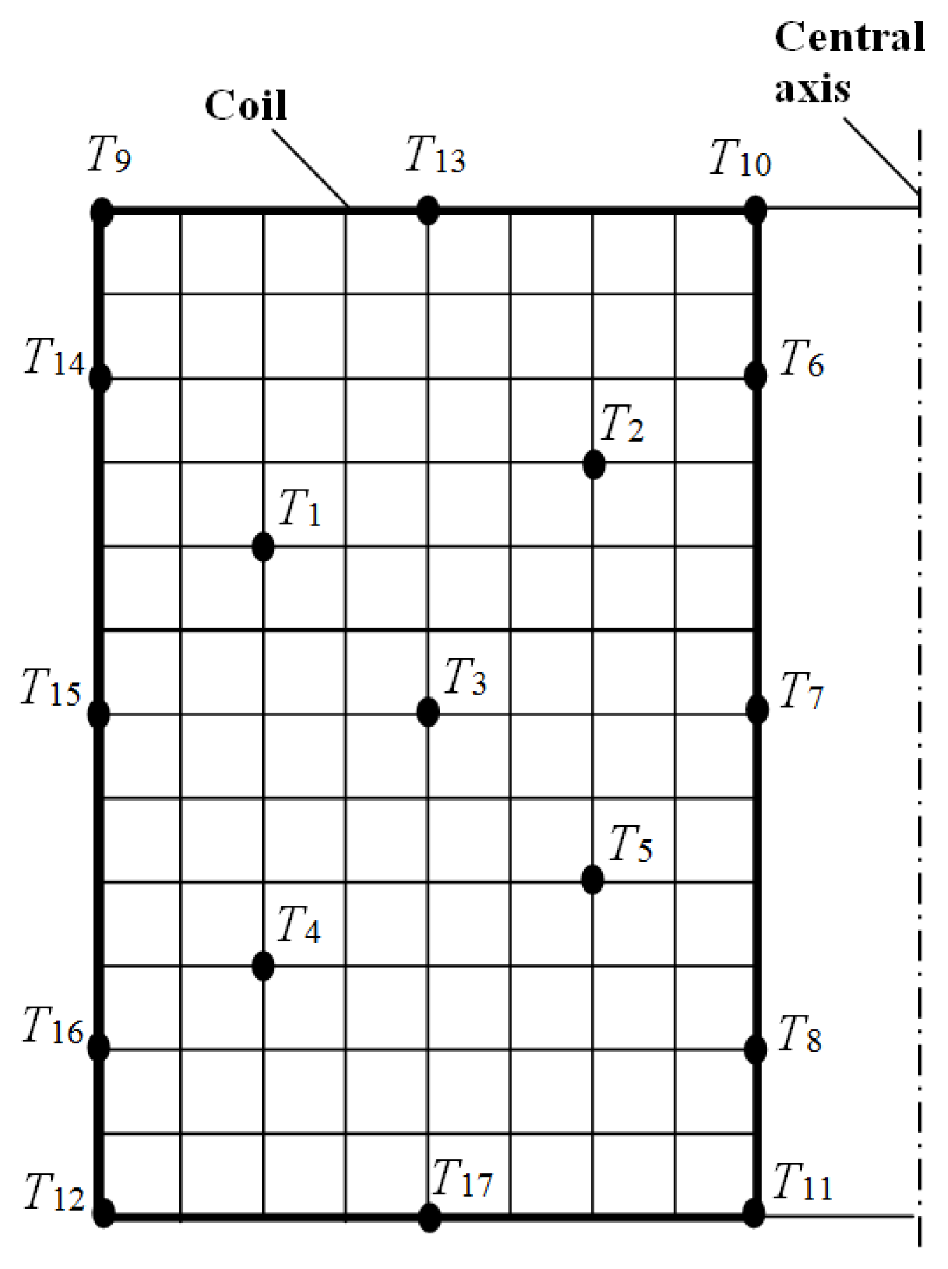Figure 4 shows measuring points of temperatures (i.e., $T_1$, $T_2$, ⋯, and $T_{13}$) in the section of annealed coil using a two-dimensional network. There were annealed coils with a sheet thickness of 0.656, 0.706, 0.805, 0.905, 1.296, and 1.524 mm.

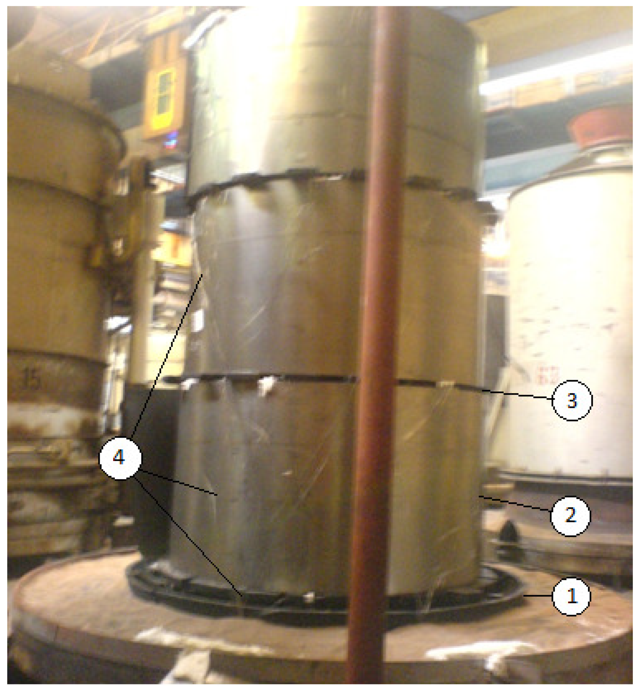
For illustration, the connections of the thermocouples are shown in Figure 5. Figure 5 shows the connection of thermocouples on coils for one operational measurement (i.e., in the annealing process). All 13 thermocouples could not be placed at each measurement so as to prevent damage. When handling the coil (i.e., laying the coil on the stand or laying the convective pad by crane, some damage of the thermocouples occurred in some measurements. Furthermore, damage could occur when placing the protective cover and furnace cover (e.g., cut off), because thermocouples were led beneath these covers. Reliability of thermocouples after measurement was assessed visually (i.e., mechanical damage-gashed thermocouple) and through the control measurement of the static characteristic of the sensor (thermocouples). From this analysis, defective thermocouples were excluded in model’s creation.

3.2. Thermophysical Properties of the Annealed Material

Heat conduction in the batch is greatly affected by the following criteria in practice:

• The chemical composition of the batch;
• The batch inhomogeneity;
• The dimensions of the batch.

The thermophysical properties of the examined materials are expressed in these criteria. The values of the thermophysical properties such as thermal conductivity, specific heat, and density of the annealed steel in laboratory and operational measurements are shown in

Table 1. Thermophysical properties of the steel.

t	0	50	100	150	200	250	300	350	400	450	500	550	600	650
$\lambda$	65.1	62.65	60.2	57.9	55.6	53.25	50.9	48.7	46.5	43.75	41	39.2	37.4	35.7
c	476	485	494	513	532	548.5	565	588	611	646.5	682	726	770	813.5
$\rho$	7875	7860.5	7846	7830	7814	7797.5	7781	7763	7745	7726.5	7708	7688	7668	7648

where t is the temperature (°C), $\lambda$ is the thermal conductivity (W·m${}^{-1}·$K${}^{-1}$), c is the specific heat (J·kg${}^{-1}·$K${}^{-1}$), and $\rho$ is the density (kg·m${}^{-3}$). These values are taken from tables for steel with a similar composition. Another important factor is the composition of the annealing atmosphere (i.e., Hydrogen-Nitrogen (HNX) mix gas). The HNX gas ratio consists of hydrogen (i.e., H${}_2$ in the range from 3% to 30%) and nitrogen (i.e., N${}_2$ in the range from 70% to 97%). In laboratory measurements, the annealing atmosphere was caused by the ratio of oxygen (i.e., O${}_2$ in the range from 2% to 21%) and nitrogen (i.e., N${}_2$ in the range from 79% to 98%) [23].

3.3. The System of Indirect Temperature Measurement

This system is based on the system of indirect temperature measurement described in [1], which includes two subsystems.

The first subsystem, i.e., system for indirect measurement of surface temperatures (SIMST) calculates (i.e., indirectly measures) the coil surface temperature from measuring the annealing atmosphere temperature $T_A$. In [1], the SIMST is realized by two models, i.e., the differential equation model and the neural network model. The differential equation model was used for the realization of SIMST. 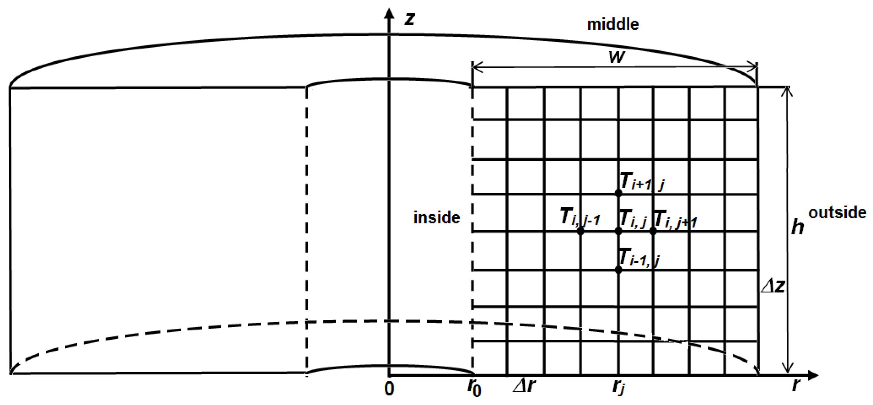This model includes coefficients (i.e., $b_k$, $k=1,2,\cdots ,5$) which were determined for three sections of the coil’s surface area, i.e., the outside surface, the inside surface, and the middle surface as shown in in Figure 6. The model has the following structure [1]:

$$\begin{array}{c}\hfill T{p}_i\left(k+1\right)=b_0+b_1·T_A\left(k+1\right)+b_2·T_A^2\left(k+1\right)+\\ \hfill +b_3·T_A\left(k\right)+b_4·T_A^2\left(k\right)+b_5·v_{term,i}·F_0\left(k+1\right)\end{array}$$

(1)

where $T{p}_i$ is the i-th coil surface temperature ($i=1,...,n$) (K), $b_0,b_1,b_2,b_3,b_4,b_5$ are the coefficients of the differential equation, $T_A$ is the annealing atmosphere temperature (K), k is the time step, n is the surface temperature count, $F_0$ is the Fourier non-dimensional criterion, and $v_{term,i}$ is the height of the i-th coil surface temperature (m).

The second subsystem, i.e., system for indirect measurement of inner temperatures (SIMIT) calculates (i.e., indirectly measures) the coil inner temperatures from the calculated (i.e., by using SIMST) coil surface temperatures. In [1], the SIMIT is realized by the two-dimensional solution of the Fourier partial differential equation of the heat conduction expressed in the orthogonal coordinates system. This equation is solved by the elementary balance method. The SIMIT was modified by adjusting the two-dimensional solution of the Fourier partial differential equation of the heat conduction to the cylindrical coordinates system, where the temperature T (K) is a function of spatial coordinates r (m), z (m), and time $\tau$ (s). In the case of two-dimensional heat conduction at the condition, the heating of the coil is all around the perimeter is the same:

$$\frac{\partial T}{\partial \tau }=\frac{\lambda }{\rho ·c}\left(\frac{1}{r}\frac{\partial }{\partial r}\left(r\frac{\partial T}{\partial r}\right)+\frac{{\partial }^{2}T}{\partial z^2}\right) \mathrm{for} r_0<r<w,0<z<h \mathrm{and} \tau >0$$

(2)

where c is the specific heat capacity of the steel coil (J·kg${}^{-1}·$K${}^{-1}$), $\rho$ is the steel coil density (kg·m${}^{-3}$), $\lambda$ is the steel coil thermal conductivity (W·m${}^{-1}·$K${}^{-1}$), and h and w are the height and width of calculated part of steel coil (see Figure 6) (m).

The initial condition for the Fourier partial differential equation of the heat conduction was considered in the following form:

$$T(r,z,0)=T_p \mathrm{for} r_0\le r\le w \mathrm{and} 0\le z\le h$$

(3)

where $T_p$ is the initial temperature (K).

The boundary condition for the Fourier partial differential equation of the heat conduction was determined in the form of the first type where are known surface temperatures (i.e., the output from SIMST).

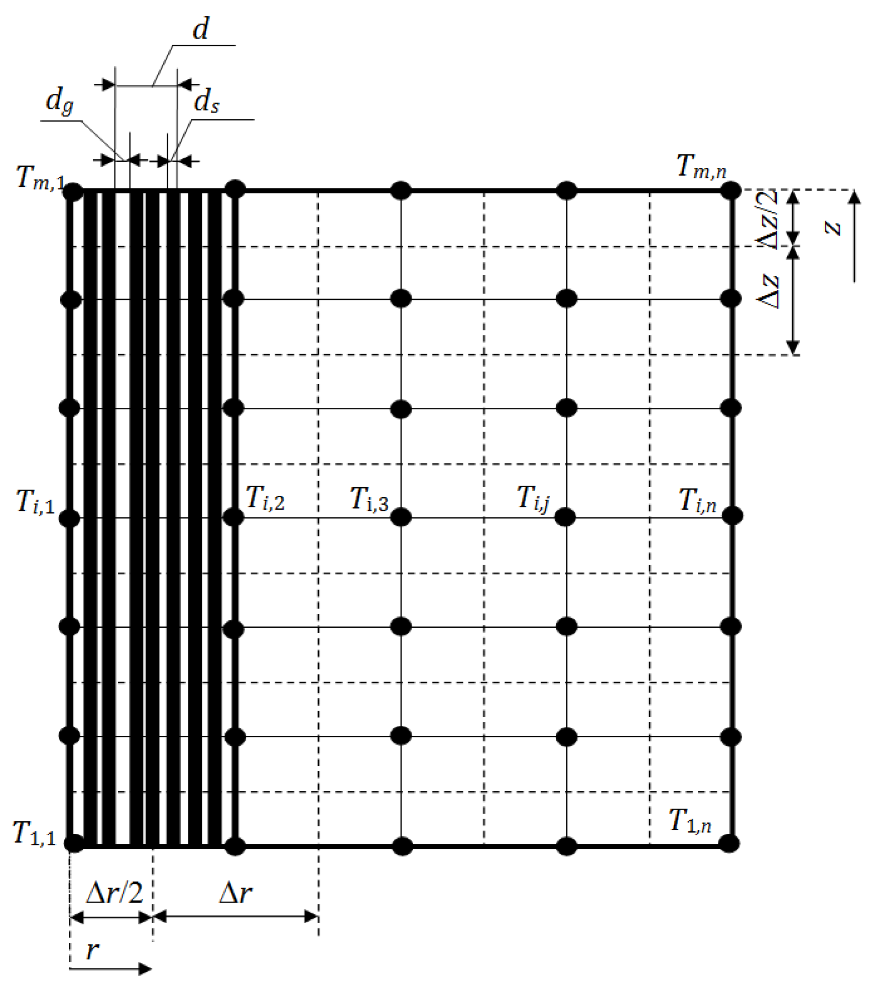
For the solution of SIMIT in the form of the Fourier partial differential equation, the finite difference method is used. On the investigated object, which is a steel coil, a network is created (see Figure 6), which is produced by guiding the parallel lines with the coordinate axes in the distance $\Delta r$ in the direction of the r-axis and at the distance $\Delta z$ in the direction of the z-axis. The temperature is defined at the individual nodal points of the coordinate system where i is the point index in the z-axis direction, j is the point index in the r-axis direction, and k is the time step. So $T_{i,j,k}$ is the temperature at the node that lies at the intersection of the i-th parallel line with the z-th coordinate, and the j-th parallel line with the r-th coordinate at time $\tau =k·\Delta \tau$ [1,3,24,25]. The temperature in the following time step $T_{i,j,k+1}$ can be determined using the following equation:

$$\begin{array}{cc}\hfill T_{i,j,k+1}& =\left(\frac{a_{r2}·r_{j+1}·\frac{T_{i,j+1,k}-T_{i,j,k}}{\Delta r}-a_{r1}·r_{j-1}·\frac{T_{i,j,k}-T_{i,j-1,k}}{\Delta r}}{r_j\Delta r}\right)·\Delta \tau +\hfill \\ \hfill \hspace{1em}& +\left(\frac{a_{z2}·\frac{T_{i+1,j,k}-T_{i,j,k}}{\Delta z}-a_{z1}·\frac{T_{i,j,k}-T_{i-1,j,k}}{\Delta r}}{\Delta z}\right)·\Delta \tau +T_{i,j,k}\hfill \end{array}$$

(4)

where ${\dot{r}}_{j+1}$ is the position between the temperature points $T_{i,j+1,k}$ and $T_{i,j,k}$ in r-axes direction, ${\dot{r}}_{j-1}$ is the position between the temperature points $T_{i,j-1,k}$ and $T_{i,j,k}$ in r-axes direction, $a_{r1}$ and $a_{r2}$ are the thermal diffusivity coefficients in r axes direction, and $a_{z1}$ and $a_{z2}$ are the thermal diffusivity coefficients in z-axes direction.

Seeing that the batch is anisotropic (i.e., non-uniform size of the gaps between threads), the finite difference method was modified, so that it was possible to determine different thermal conductivity in the direction of the r- and z-axis. Values of thermal conductivity depending on the thickness of the gap were used in the direction of the r-axis. Values of thermal conductivity depending on the chemical composition of the steel were used in the case of the direction of the z-axis.

3.4. The Proposal of Optimization Methods for Estimating Thermophysical Properties

The heat is transferred from the coil surface to the inside, mainly through the conduction, but due to the presence of gaps between the coil windings. A simple model is not adequate for describing the heating inside the coil. Therefore, an effective radial thermal conductivity for modeling the distribution of heat inside the coil is usually used. In an ideal coil, heat is transferred in the radial direction through the alternating layers of steel and the annealing gas. Other factors that influence the effective radial conduction in real coil are the following:

• Variable surface roughness of sheets;
• Thermal radiation adding another factor to the radial heat transfer in the coil.

In general, the total radial conductivity is the set of functions dependent on many parameters such as specific heat, thermal conductivity, density, temperature gradient, and the strength of coil, as well as the properties of the filling gas (i.e., thermal conductivity and density). The model that has solved the effective radial thermal conductivity can be defined in terms of the conductivity of steel coils and filling gas and their relative ratio using the following equation [1]:

$${\lambda }_u=\frac{d_s+d_g}{\frac{d_s}{{\lambda }_s}+\frac{d_g}{{\lambda }_g}}$$

(5)

where ${\lambda }_u$ is the thermal conductivity layers of steel and gas (W·m${}^{-1}·$K${}^{-1}$), ${\lambda }_s$ is the thermal conductivity of steel (W·m${}^{-1}·$K${}^{-1}$), ${\lambda }_g$ is the thermal conductivity of filler gas (W·m${}^{-1}·$K${}^{-1}$), $d_s$ is the average thickness of metal sheet of coil (m), and $d_g$ is the average thickness of the coil’s gap (m).

The following equation was used to calculate the thickness of the gap where the measurement of individual values is shown in Figure 7:

$$d_g=\frac{d-N·d_s}{N-1}$$

(6)

where $d_g$ is the thickness of the gap between the threads (m), $d_s$ is the sheet thickness wound steel coil (m), d is the distance of the measured area (m), and N is the number of windings in the selected area that is measured.

The task was to develop a system of indirect measurement, which in terms of measurement accuracy will be at least equivalent to measurement in using the current industrial measurement systems. For this purpose, the system of indirect temperature measurement was extended with optimization methods. These methods enable to determine following thermophysical parameters:

• Thermal diffusivity a as a function of temperature and following thermal conductivity layers of steel and gas ${\lambda }_u$. Thermal diffusivity in the direction of r-axis is considered in the following form:

  $$a=\frac{{\lambda }_u}{\rho ·c}$$

  (7)

  where ${\lambda }_u$ is the thermal conductivity layers of steel and gas (W·m${}^{-1}·$K${}^{-1}$), c is the specific heat of steel (J·kg${}^{-1}·$K${}^{-1}$), and $\rho$ is the density of steel (kg·m${}^{-3}$);
• Thermal conductivity of filler gas ${\lambda }_g$.

The main task of the proposed optimization methods is determining optimal values of selected parameters (i.e., thermal diffusivity and thermal conductivity) for objective function extremalization.

3.4.1. Objective Function

The system of indirect temperature measurement (SIMT) is ultimately a simulation model, which based on partial mathematical models can dynamically predict and indirectly measure output variable (i.e., the temperature of the batch). In terms of the utilization of the created model, it is necessary to assess its qualitative and quantitative adequacy. Review the adequacy of the model is the comparison of simulation results with experimental data measured on a real object. Identified deviations are used for the model’s correction. This procedure is the only possibility to test the quantitative and to some extent the qualitative adequacy of the model. The qualitatively adequate model represents process laws in the given field. It means that the character of the simulated behavior of the process and the real behavior of the process is the same, but the values of variables may not be the same. At the quantitative adequacy, a difference between the real $x_r$ and simulated $x_m$ course of the process is within allowable limits $\epsilon$ in all fields of the model application:

$$|x_r-x_m|\le \epsilon$$

(8)

The simulation model should predict the information with at least such accuracy as is required by production technology. This simulation model can be adapted by the modification of its ambiguously determined input variables (e.g., thermophysical properties). The task of adaptation is to minimize the quantitative model weaknesses to the required accuracy $\epsilon$.

Adaptation algorithms for determining thermal-physical properties are based on the principle of the optimization method. The aim is to minimize the objective function that is expressed by the sum of quadrates of deviation between measured temperatures on the real object and temperature obtained from SIMT (i.e., simulation model). The form of the objective function for minimizing the deviation of one temperature of steel coil is as follows:

$$F={\displaystyle \sum _{p=1}^l}{\displaystyle \sum _{z=1}^k}{\displaystyle \sum _{j=1}^s}{(T_{j,z,p}^{measured}-T_{j,z,p}^{SIMT})}^2$$

(9)

where $T_{j,z,p}^{measured}$ is the temperature measured in the batch on the real object (bell furnace), $T_{j,z,p}^{SIMT}$ is the model temperature (i.e., output variable from the SIMT model), j is the index of temperature in the coil, s is the number of directly measured inner temperatures, z is the time step of simulation, k is the total time step of simulation, p is the number of measurement, and l is the count of measurements.

3.4.2. The Proposal of the Method for Estimating the Thermal Diffusivity a

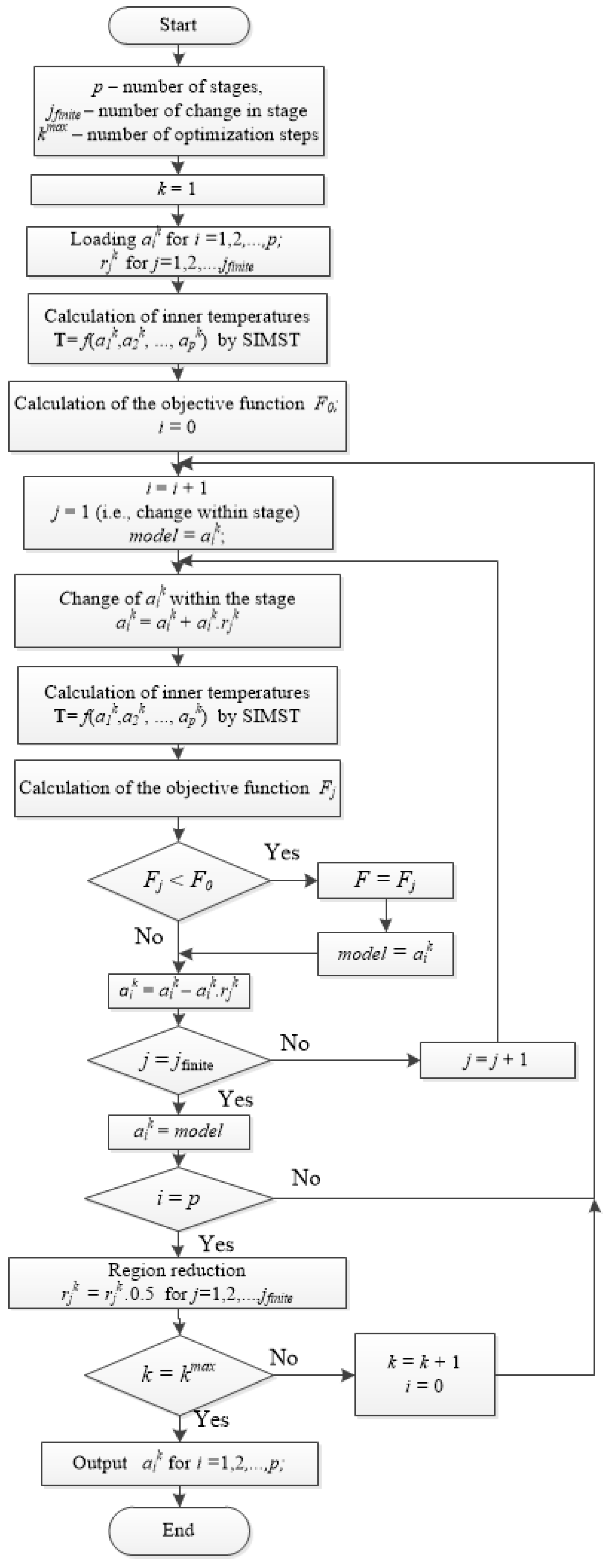
The core of determination of thermal diffusivity a in SIMT is the optimization algorithm, which is based on the principle of iterative dynamic programming (IDP). The process is divided into p time periods. In the first stage, an approximate optimum is found, then continues to the next stage wherein optimization is the first stage considered as a known and optimal. This procedure is repeated up to the final stage. Found trajectory is then used as the initial estimation in the next iteration of optimization. Every iteration ends with a decrease of the region of control in which optimum is searched. This sequence is repeated for a given amount of iterations $k_{max}$ [26,27]. In order to avoid optimization in infinite space of all possible controls at the beginning of each iteration is generated by $j_{finite}$ different trajectories of control evenly spaced in the space around the best estimation of the optimal trajectory.

In our case, dividing the process in terms of temperature (i.e., behavior of thermal diffusivity $\overline{a}\Rightarrow a_i$ for $i=1,2,...,p$) on p stages. In the initial estimation thermal diffusivities are tabulated for $\Delta T=100{}^{\circ }$C. Following, determining the vector of changes $\overline{r}$ that contains $j_{finite}$ changes (i.e., thermal diffusivity trajectories ) within the i-th stage. The determination of optimal trajectory of i-th stage is realized by calculation of the objective function (9) using of SIMT for each trajectory. Optimal trajectory (i.e., thermal diffusivity) has the minimal value of the objective function. At each new iteration, the reduction of the region for setting the variable occurs (i.e., area of setting) for thermal diffusivity. The problem may occur in the length of the adaptation algorithm. The modified adaptation algorithm for determining thermal diffusivity a in the form of a flow diagram is shown in Figure 8.

3.4.3. The Proposal of the Method for Estimating the Thermal Conductivity of Filler Gas ${\lambda }_g$

The algorithm for determining the thermal conductivity of filler gas ${\lambda }_g$ is based on the principle of the gradient method. The aim is to minimize the objective function F (9), expressed by sum of quadrates of deviation between the measured internal temperatures on the real object (i.e., steel coil) and temperatures obtained from the system of indirect temperature measurement (SIMT) (i.e., simulation model) by the utilization of the finite differences method. The equation in which thermal conductivity layers of steel and gas ${\lambda }_u$ was used in calculations of this method for thermal conductivity in the direction of the r-axis. This equation takes into account the thickness of the sheet, the thickness of the gap, the thermal conductivity of steel ${\lambda }_s$, and thermal conductivity of optimized filling gas ${\lambda }_g$.

The generalized iterative algorithm of the gradient method for minimizing the objective function has the form [28]:

$${\overline{x}}^{i+1}={\overline{x}}^i-h·gradF\left({\overline{x}}^i\right)$$

(10)

where h is the constant of iteration (step), which select in such a way so that the values of ${\overline{x}}^{i+1}$ would not distort conditions of existence of function $F\left(\overline{x}\right)$ and also was fulfilled (in minimization) following: $F\left({\overline{x}}^{i+1}\right)<F\left({\overline{x}}^i\right)<\cdots <F\left({\overline{x}}^1\right)<F\left({\overline{x}}^0\right)$.

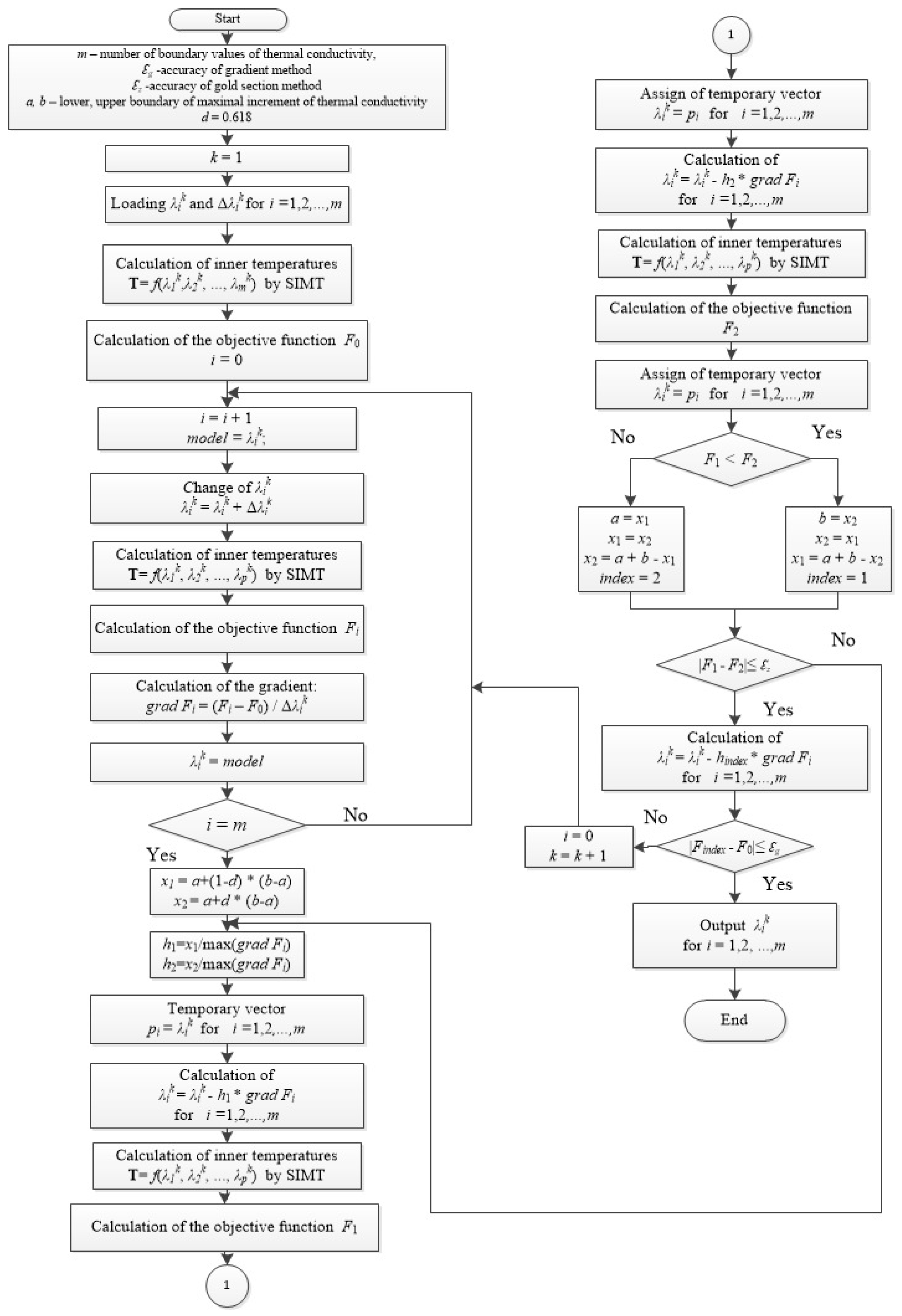
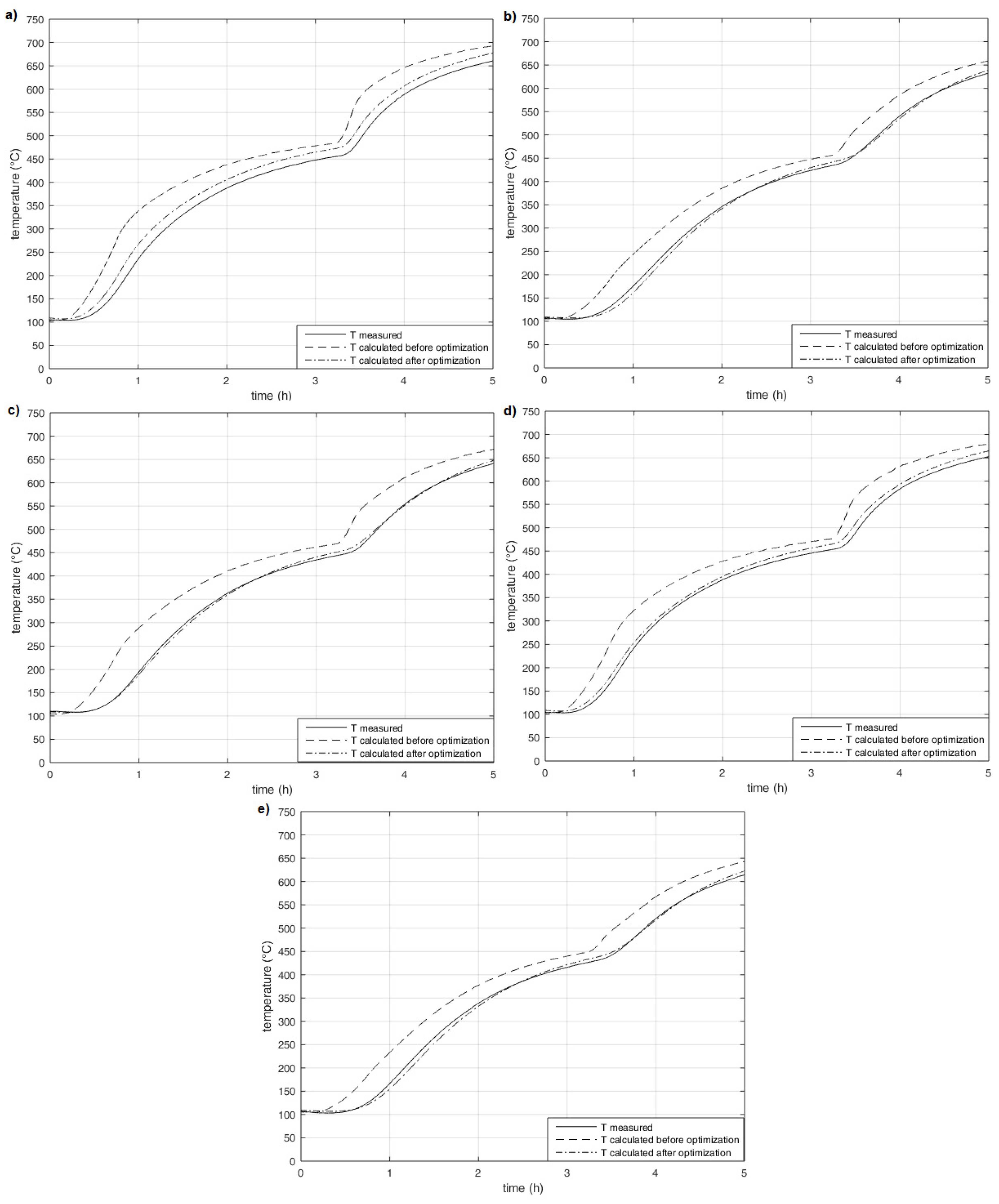
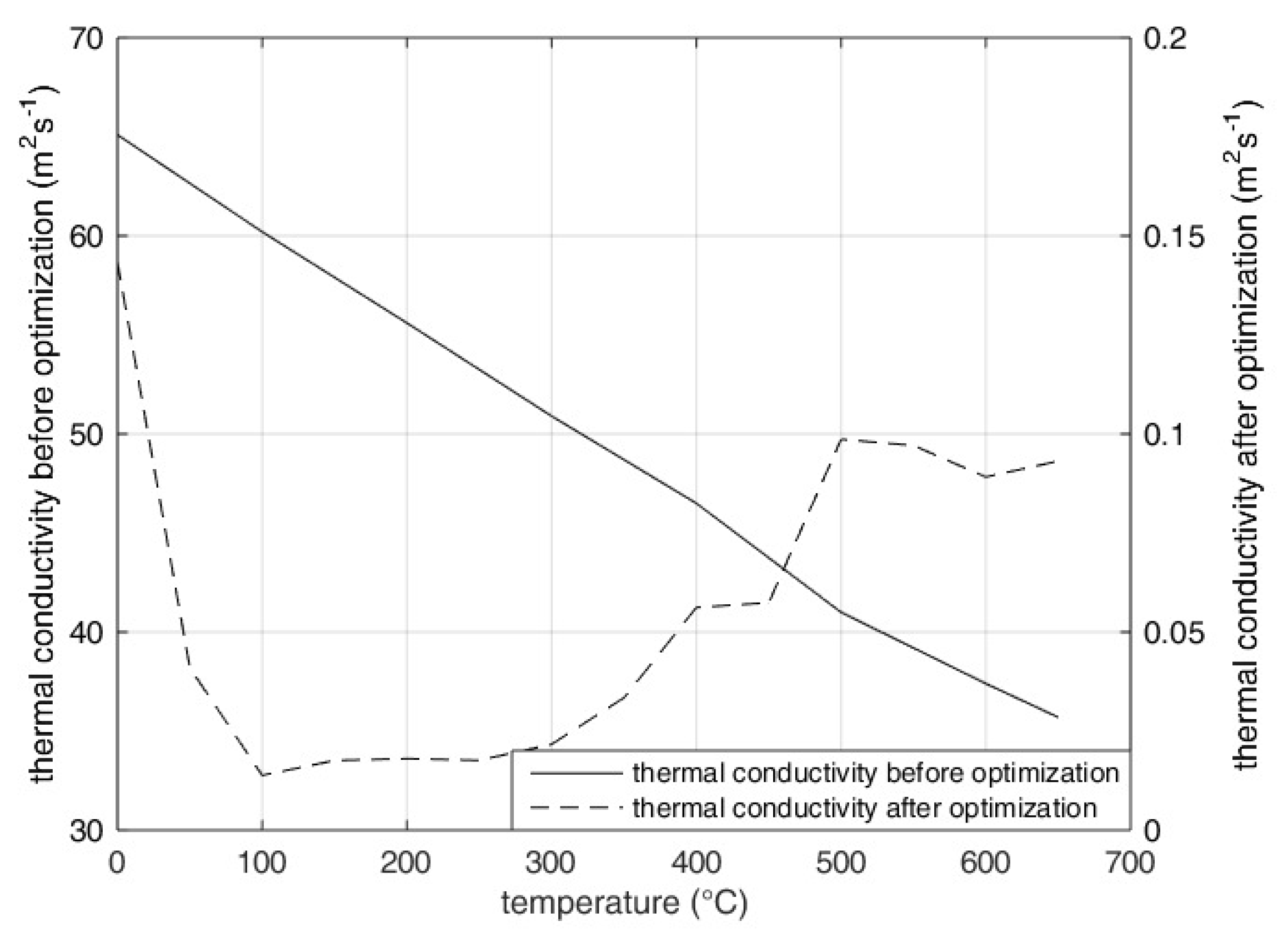
The values of vector $\overline{x}$ were considered as values of thermal conductivity of filler gas ${\lambda }_g$ marked following as $\overline{\lambda }$. The value of thermal conductivity of filler gas $\overline{\lambda }$ (in selected boundary temperatures—graded by 50 °C) i.e., ${\lambda }_i$ for i = 1, 2, ⋯, m (m is the number of boundary temperatures—the number of components of the vector $\overline{x}$), and $\Delta \overline{\lambda }$ (the change of $\overline{\lambda }$) were considered as inputs. Step h of the gradient method was optimized by the golden section method to increase the efficiency of the selected optimization method (reducing the time of simulation and improve the accuracy of the solution). During optimization, the values of thermal conductivity in r-direction were determined for individual temperature ranges. The value of thermal conductivity in z-direction remained unchanged. It had values of thermal conductivity of steel.

The algorithm of the gradient method for determining the thermal conductivity of filler gas with step h obtained from the golden section method is shown in Figure 9.

4. Results and Discussion

4.1. The Verification of the Method for Estimating the Thermal Diffusivity

In the objective function, five internal temperatures and 11 measurements occurred because the optimization of thermal diffusivity was performed on 11 laboratory measurements. The behavior of thermal diffusivity before and after optimization is shown in Figure 10. The value of thermal diffusivity before optimization was determined by calculation according to Equation (7), but instead of the thermal conductivity layers of steel and gas, the thermal conductivity of steel was used. The visible decline of the thermal diffusivity value after optimization is shown in Figure 10.

Figure 11 (i.e., the values for measurement 1) and Figure 12 (i.e., the values for measurement 11) show a comparison of directly measured and indirectly measured (i.e., calculated by SIMT) inner temperatures $T_1,\dots ,T_5$ before and after optimization of thermal diffusivity. The behavior of the indirectly measured temperature after optimization is obtained by optimized thermal diffusivity. In these figures, not only are qualitative but also the quantitative approximation of the indirectly measured (i.e., calculated) temperature to the directly measured temperature can be seen.

The accuracy of SIMT was calculated as a relative deviation of the indirectly measured temperature from the directly measured temperature according to the following equation:

$${\delta }_j=\frac{\frac{{\sum }_{z=1}^{k}abs(T_z^{measured}-T_z^{SIMT})}{T_z^{measured}}·100}{k}$$

(11)

where ${\delta }_j$ is the relative deviation of the j-th temperature, j is the index of temperature in the coil, z is the time step of simulation, and k is total time step of the simulation.

Figure 11 and Figure 12 show that approximation at temperatures $T_2,\dots ,T_5$ has sufficient accuracy. This result is confirmed by

Table 2. Average relative deviation of system of indirect temperature measurement (SIMT) for laboratory measurement.

Measurement	$\mathit{\delta }$ (%)
	T${}_1$	T${}_2$	T${}_3$	T${}_4$	T${}_5$
1	6.9	5.1	4.4	3.2	4.6
2	6.7	4.7	5.6	3.1	3.8
3	6.0	4.2	5.9	4.2	4.4
4	3.3	2.4	2.8	1.8	2.0
5	6.3	4.4	6.3	4.2	4.6
6	3.3	2.4	3.1	2.3	2.4
7	3.5	2.5	3.3	2.5	2.6
8	3.6	2.6	3.3	2.5	2.6
9	3.6	2.5	3.3	2.5	2.6
10	5.9	3.9	5.8	4.3	4.3
11	5.5	3.3	2.4	4.3	3.9

. Table 2 shows the results of the accuracy of SIMT in the optimal determination of thermal diffusivity of 11 laboratory measurements.

The visible differences in Figure 11, Figure 12, and Table 2 can be caused by:

• Different thickness of gaps after a cross-section of the coil, i.e., thermal diffusivity, in this case, can be also the function of distance from $r_0$ to outside of the coil, eventually, look for the function of the gap thickness between the windings along the coil cross-section (i.e., the function of the gaps position, the annealed sheet thickness, and the coil volume);
• Were used as approximate table values for thermal conductivity of the layers of steel;
• Measurement error at directly measured temperatures on the outer surface of the coil, at those locations the highest temperatures were measured. This error can affect the approximation of the temperatures at the grid points between the directly measured temperatures (i.e., in the calculation of the final difference method).

4.2. The Verification of the Method for Estimating the Thermal Conductivity of Filler Gas

In the objective function, three inner temperatures and seven operational measurements occurred because the optimization of thermal conductivity of filler gas was realized on seven operational measurements. The entry into SIMT was the temperature of the atmosphere directly measured in these operational measurements and calculated inner temperatures were as the output. These calculated inner temperatures were regarded as inputs to the objective function.

Figure 13 compares the behavior of the filler gas’s thermal conductivity before and after optimization. Thermal conductivity values of the filler gas before optimization were set up for thermal conductivity of the steel layer. From Figure 13, the decrease of thermal conductivity values after optimization is visible. This decrease was caused by the lower thermal conductivity of HNX gas toward the thermal conductivity of the steel layer. In case of considering heat transfer by the radiation and the convection between windings of the coil (gas layer), the sum of the heat flow does not reach the amount of heat flow of conduction in the steel layer.

Figure 14, Figure 15 and Figure 16 show a comparison of directly measured and indirectly measured (i.e., calculated by SIMT) inner temperatures $T_6$, $T_7$, and $T_8$ before and after optimization of thermal conductivity.

The behavior of the indirectly measured temperature after optimization is obtained by optimized thermal conductivity. In these figures, not only is the qualitative shown but also the quantitative approximation of indirectly measured (i.e., calculated) temperature to directly measured temperature. Similarly, as in the section of thermal diffusivity optimization, the worst approximation is at the temperature measured closest to the outside surface of the coil. In case of optimization of thermal conductivity, it is the temperature $T_6$. Figure 14, Figure 15 and Figure 16 show that approximation at temperatures $T_7$ and $T_8$ had sufficient accuracy. This result is confirmed by

Table 3. Average relative deviation of SIMT for operating measurements.

Measurement	Coil	$\mathit{\delta }$ (%)
		T${}_6$	T${}_7$	T${}_8$
1	Coil #2	4.4	1.9	1.2
	Coil #3	4.6	2.5	2.9
2	Coil #2	4.1	2	2.4
	Coil #3	4.5	1.5	3.2
3	Coil #1	6.3	2.8	3.2
	Coil #2	3.6	5.1	1.4
4	Coil #1	8.4	6.2	7.5
5	Coil #1	6.8	4.7	5.8
	Coil #2	8.1	4.3	5.4
6	Coil #2	-	8.6	13.5
7	Coil #1	10.9	4.8	-

. Table 3 shows the results of the accuracy of SIMT calculated according to Equation (11) in the optimal determination of thermal conductivity of seven operating measurements.

It can be assumed that the input settings closer to reality would reduce the number of optimization steps (i.e., duration of optimization) and reduce differences between behaviors directly and indirectly measured temperatures.

The quality of annealed coils in terms of temperature regime is given by the condition that even the minimum temperature in the annealed coil should reach re-crystallization temperature. If this temperature is not reached, then the annealing quality is not satisfactory. This temperature was marked as “cold spot” and for operating measurements is shown in

Table 4. The time from cold spot temperature reach to holding time ending for operating measurements.

Measurement	Coil	Cold Spot (°C)	Maximum (°C)	Time (h)
1	Coil #2	620	665.4	8.5
	Coil #3	620	673.2	9.2
2	Coil #2	530	557.8	7.3
	Coil #3	530	566.4	8.2
3	Coil #1	670	699.1	13.1
	Coil #2	670	708.6	11.4
4	Coil #1	680	709.5	14.6
5	Coil #1	680	707.4	16.2
	Coil #2	680	729.6	23.3
6	Coil #2	630	693.7	17.5
7	Coil #1	630	684.6	7.8

. The highest temperature reached in the coldest place of the coil (i.e., maximum) and the time from cold spot temperature reached to holding time ending (i.e., time) is also shown in this table. Calculations have shown (see Table 4) that the cold spot temperature was always reached, i.e., the holding time was longer than necessary. The proposed system could, in running operation, check that the cold spot temperature was achieved in each coil and consequently adjust the holding time. A possible reduction of holding time could bring savings of mixture gas, energy savings for annealing furnaces, etc.

4.3. Application of SIMT in the Laboratory Bell Furnace

SIMT with optimal values of thermal conductivity was used for the online visualization of the estimated annealed coil inner temperature. This temperature was compared with the directly measured annealed coil inner temperature.

For the online visualization of the inner annealed coil temperatures, it is necessary to create a monitoring system or to extend the existing control system of bell furnace with a subsystem for calculating and visualizing internal coil temperatures. This change also allows the prediction of the internal temperature of the annealed coil in the given annealing regime. The staff of the annealing plant with bell furnaces, based on the internal temperature information, can effectively control the annealing process (i.e., the annealed batch quality and process failure flexibility).

The used monitoring system was developed as the desktop application for PC with MS Windows. The monitoring system is programmed in Delphi IDE and enables one to monitor all directly measured temperatures through text fields and graphs. It is also able to run external application i.e., program realization of the mathematical model (OnlineSimulation.exe) for calculation of indirectly measured temperatures inside the coil. The main screen of the monitoring and control system is shown in Figure 17. This figure also shows a comparison of directly and indirectly measured temperature in a selected position of the annealed coil. The proposed monitoring system is connected with PLC by the OPC protocol.

5. Conclusions

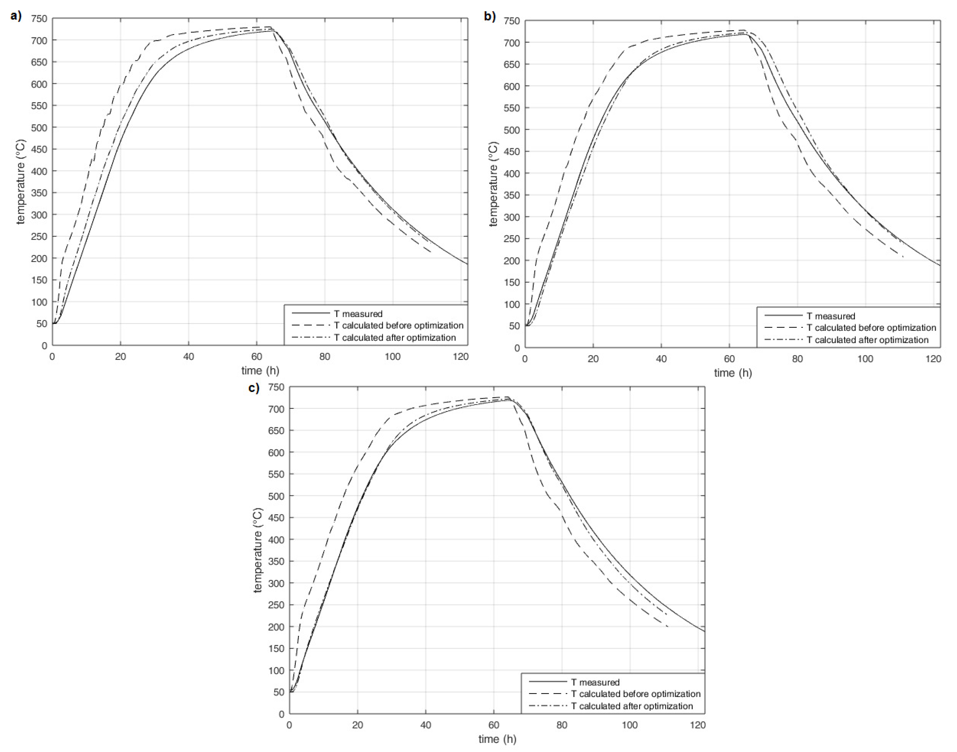
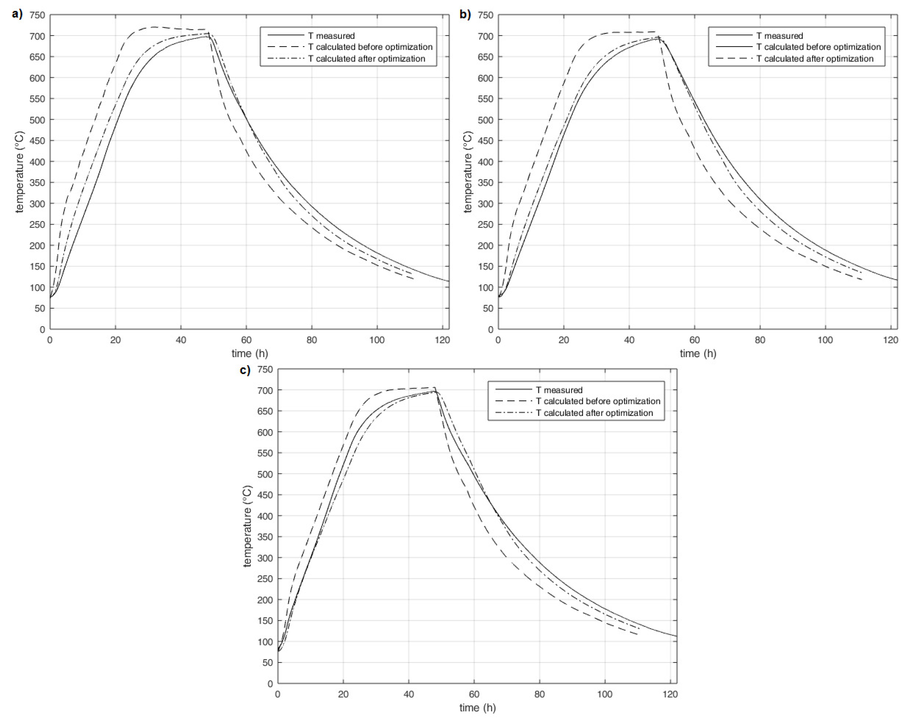
The paper dealt with the application of optimization methods to estimate thermophysical parameters such as thermal diffusivity and thermal conductivity, to improve the accuracy of temperatures’ indirect measurement in the annealing process. Nowadays, some methods for solving nonlinear optimization problems in the field of heat treatment of materials determine the resulting optimized parameters in the form of a constant for the entire material processing-cycle or its phase (i.e., heating, holding, or cooling). In addition, more expensive hardware is used (i.e., pyrometers, thermographic cameras, etc.) and laboratory trials are needed. The proposed solution differs from these methods as it applied two optimization methods (i.e., IDP method and gradient method) for multi-dimensional optimization (i.e., determination of thermal conductivity or thermal diffusivity values at specified boundary temperatures). The IDP method was applied for the optimization of thermal diffusivity in the direction of the r-axis in laboratory conditions. The gradient method was applied for the optimization of thermal conductivity of filler gas, which was used for the calculation of the effective thermal conductivity in r-direction. The results show that both methods were suitable for the application to the SIMT according to the comparison of directly (i.e., by thermocouples) and indirectly (i.e., by simulation model) measured temperatures. Within the optimization of thermal diffusivity, the highest value of the relative deviation (i.e., 6.9%) was reached in temperature $T_1$, and the lowest value of the relative deviation (i.e., 1.8%) was reached in temperature $T_4$. The temperature $T_4$ was placed nearer to the coil’s central axis. Within optimization of thermal conductivity, the highest value of the relative deviation (i.e., 8.4%) was reached in temperature $T_6$, and the lowest value of the relative deviation (i.e., 1.2%) was reached in temperature $T_8$. The temperature $T_8$ was placed nearer to the coil’s central axis. Due to thermocouple $T_6$ in experimental measurement 6 and thermocouple $T_8$ in experimental measurement 7, measurement 6 and 7 were damaged and not included in reported results.

It can be assumed that a faster temperature rise towards the outer surface reduces optimization efficiency in contrast to internal temperatures and temperatures oriented in a direction towards the inner surface where the temperature rise/fall is milder. Due to the inaccuracy of SIMT at the temperature measured close to the outside surface of the coil, it would be desirable to determine the dependence of thermal diffusivity and thermal conductivity considering the position from the central axis of the coil. Deviations in operating measurements can be caused by the use of tabulated values of thermal conductivity, heat capacity, and density, which was found only approximately for the annealed type of steel. It can be assumed that if there were more precise values of thermophysical properties of steel, the behavior of thermal conductivity of filler gas would respond more to its real values. Determining more accurate values of optimized thermal conductivity could also be achieved in case of the gradient method extension using the Newton method of the second order. This method is more effective near the extreme. First, a gradient method would be used, and in the case of looping iterations around an extreme point, a Newton method of second-order would be used.

In case of visualization of the calculated inner temperature, it is a possible visual check of annealing process state. Based on this visual check, it is possible to modify the course of annealing curves in the case that the inner temperature of the coil does not have the required behavior. The advantages of the proposed solution are the following:

• The proposed model does not work with tabulated values of thermophysical properties in running operation, but with values optimized for the process;
• Possibility of the visualization of temperature field through cross-section of annealed coil;
• Adjusting the annealing regime to the needs of the annealed batch (i.e., in emergency or failure regime);
• Proposal of new control methods where the controlled value would not be the temperature of the annealing atmosphere, but the inner temperature estimated by the indirect measurement system.

The annealing time is currently determined experimentally for the specific type and thickness of the annealed steel. Information about the inner temperature in the annealed coil could optimize the cost of the annealing process by shortening the annealing time (i.e., if the recrystallize temperature was reached in the total annealed coil volume rather than original annealing modes used) and/or reducing faulty goods.