Data-Driven Model-Free Adaptive Control Based on Error Minimized Regularized Online Sequential Extreme Learning Machine

Abstract

Model-free adaptive control (MFAC) builds a virtual equivalent dynamic linearized model by using a dynamic linearization technique. The virtual equivalent dynamic linearized model contains some time-varying parameters, time-varying parameters usually include high nonlinearity implicitly, and the performance will degrade if the nonlinearity of these time-varying parameters is high. In this paper, first, a novel learning algorithm named error minimized regularized online sequential extreme learning machine (EMREOS-ELM) is investigated. Second, EMREOS-ELM is used to estimate those time-varying parameters, a model-free adaptive control method based on EMREOS-ELM is introduced for single-input single-output unknown discrete-time nonlinear systems, and the stability of the proposed algorithm is guaranteed by theoretical analysis. Finally, the proposed algorithm is compared with five other control algorithms for an unknown discrete-time nonlinear system, and simulation results show that the proposed algorithm can improve the performance of control systems.

1. Introduction

It is difficult to obtain an accurate mechanism model of a physical system when the production technologies and processes are very complex. Data-driven control (DDC) [1] relies on input/output (I/O) data of control systems and does not need to consider mechanism models of systems. After several years of development, some data-driven control techniques have been investigated, such as, proportional-integral derivative (PID) [2], fuzzy logic control [3], unfalsified control (UC) [4,5], model free adaptive control (MFAC) [6,7,8,9,10,11,12], iterative learning control (ILC) [13,14,15], iterative feedback tuning (IFT) [16,17], some control algorithms based on neural network [18,19,20,21,22,23] and so on.

MFAC is a class of DDC, and it builds a virtual equivalent dynamic linearized model [24] by using a dynamic linearization technique. The virtual equivalent dynamic linearized model contains some time-varying parameters. In practice, it is often not easy to obtain the resulting time-varying parameters, but they can be estimated by using historical data of control systems. Those time-varying parameters usually include high nonlinearity implicitly, and the performance will degrade if the nonlinearity of the resulting time-varying parameters is too severe [25]. The traditional methods of getting those time-varying parameters are projection algorithm, recursive least squares, and so on. Besides every time-varying parameter in the virtual equivalent dynamic linearized model can be considered as a nonlinear function, and in [25], radial basis function neural network (RBFNN) is used to estimate those time-varying parameters.

Extreme learning machine (ELM) is developed for offline learning and training a single-hidden-layer feed forward neural networks (SLFNs) [26]. Online sequential extreme learning machine (OS-ELM) [27] is an online learning algorithm, it adjusts the output weights online, besides the input weights and hidden biases are randomly chose. In recent years OS-ELM has gained a large amount of interests and been uesed to estimate unknown parameters of systems [28,29]. Some improved OS-ELM algorithms were introduced by some scholars, such as regularized online sequential extreme learning machine (REOS-ELM) [30], initial-training-free online extreme learning machine (ITF-OELM) [31], etc. Although, the learning speed of OS-ELM is extremely high, it could yield singular and ill-posed problens. To overcome adverse effects, which cuased by the noisy data of control systems, REOS-ELM, which is an improvement of OS-ELM, was investigated. In [30], REOS-ELM was introduced, however the stability of REOS-ELM for unknown discrete-time nonlinear systems was not analysed, and how to select the hidden node number of neural networks is unknown.

In this paper, first, a updating formula which contains dead-zone characteristics for REOS-ELM is introduced. Second, in order to obtain a more compact network structure, error minimized regularized online sequential extreme learning machine (EMREOS-ELM) is investigated, EMREOS-ELM is different from EMOS-ELM [28], and it updates the output weights using the pseudoinverse of a partitioned matrix during the growth of the networks. Finally, a novel model-free adaptive control method based on EMREOS-ELM is proposed. This paper is structured as follows, in Section 2 REOS-ELM is briefly introduced. Dynamic linearization technique and the updating formula which contains dead-zone characteristics for REOS-ELM are introduced in Section 3. The model-free adaptive control method based on EMREOS-ELM and the stability analysis of the proposed method for unknown discrete-time nonlinear systems are stated in Section 4. Section 5 shows simulation experiments. In Section 6 some conclusions are brought.

2. REOS-ELM

In [32], the universal approximation capability of ELM was analyzed. ELM is developed for offline learning, however training data could arrive one-by-one or chunk-by-chunk; OS-ELM is an online version of ELM, and it is sensitive to noise data; REOS-ELM is an improvement of OS-ELM. In this part REOS-ELM will be introduced.

Suppose that there is an initial training dataset with $N_0$ training patterns $({\mathit{x}}_j,t_j)\in {\mathit{R}}^n\times \mathit{R}$ where ${\mathit{x}}_j={[x_{j1},x_{j1},\cdots ,x_{jn}]}^T$. For a single hidden layer neural network with n input nodes and one output node, the jth output corresponding to the jth input pattern is

$$o_j=\sum _{i=1}^L{\beta }_{i}G({\mathit{w}}_i,b_i,{\mathit{x}}_j),j=1,\cdots ,N_0$$

(1)

where L denotes the number of hidden nodes, and the subscript i indicates the ith hidden node; $G(·)$ and $o_j$ are the active function of hidden nodes and the output of the network, respectively, $b_i$ and ${\beta }_i$ are the hidden bias of the ith hidden node and the output weight connecting the ith hidden layer and the output node, respectively.

OS-ELM is a novel online learning algorithm due to its highlighted features, and its highlighted features are that the input weights and hidden biases are randomly chose, and the main goal of training process is to determine the output weights. In order to obtain output weights, they minimize the error function defined by

$$\parallel {\mathit{H}}_0{\mathit{\beta }}_0-{\mathit{T}}_0{\parallel }^2.$$

(2)

The collected data for training process often contains noise, and the only objective of empirical risk minimization as shown in (2) may lead to poor generalization and over-fitting [30]. REOS-ELM is different from OS-ELM, and REOS-ELM tries to minimize the empirical error and obtain small norm of network weight vector [30]. In [30] the followin cost function was considered, and the cost function is

$$\parallel {\mathit{H}}_0{\mathit{\beta }}_0-{\mathit{T}}_0{\parallel }^2+\lambda {\parallel {\mathit{\beta }}_0\parallel }^2$$

(3)

where $\lambda$ is a regularization factor.

The solution of ${\mathit{\beta }}_0$ is

$${\mathit{\beta }}_0={\mathit{P}}_0{\mathit{H}}_0^T{\mathit{T}}_0,$$

(4)

and

$${\mathit{P}}_0={({\mathit{H}}_0^T{\mathit{H}}_0+\lambda {\mathit{I}}_L)}^{-1}$$

(5)

here ${\mathit{I}}_L$ is an identity matrix, the size of ${\mathit{I}}_L$ is L, ${\mathit{T}}_0={\left[t_1,\cdots ,t_{N_0}\right]}^T$, and

$${\mathit{H}}_0={\left[\begin{array}{ccc}G({\mathit{w}}_1,b_1,{\mathit{x}}_1)\hfill & \cdots \hfill & G({\mathit{w}}_L,b_L,{\mathit{x}}_1)\hfill \\ ⋮\hfill & \cdots \hfill & ⋮\hfill \\ G({\mathit{w}}_1,b_1,{\mathit{x}}_{N_0})\hfill & \cdots \hfill & G({\mathit{w}}_L,b_L,{\mathit{x}}_{N_0})\hfill \end{array}\right]}_{N_0\times L}.$$

(6)

When the kth chunk of data is recerived

$$N_k=\left\{({\mathit{x}}_i,t_i)\right\}{}_{i={\sum }_{j=0}^{k-1}{N}_j+1}^{i={\sum }_{j=0}^k{N}_j}$$

(7)

The weight updating algorithm, which is used in REOS-ELM, takes a similar form to recursive least squares (RLS) algorithm, and

$${\mathit{P}}_k={\mathit{P}}_{k-1}-\frac{{\mathit{P}}_{k-1}{\mathit{H}}_k^T{\mathit{H}}_k{\mathit{P}}_{k-1}}{{\mathit{I}}_{N_k}+{\mathit{H}}_k{\mathit{P}}_{k-1}{\mathit{H}}_k^T},$$

(8)

and

$${\mathit{\beta }}_k={\mathit{\beta }}_{k-1}+{\mathit{P}}_k{\mathit{H}}_k^T({\mathit{T}}_k-{\mathit{H}}_k{\mathit{\beta }}_{k-1})$$

(9)

where ${\mathit{I}}_{N_k}$ is an identity matrix, and the size of ${\mathit{I}}_{N_k}$ is $N_k$; ${\mathit{T}}_k$ and ${\mathit{H}}_k$ are the target of kth arriving training data and the hidden layer outputs for the kth arriving training data, respectively.

3. Dynamic Linearization Technique and the New Updating Formula for REOS-ELM

3.1. Dynamic Linearization Technique

MFAC builds a virtual equivalent dynamic linearized model by using a dynamic linearization technique.

The following unknown discrete-time nonlinear system is considered

$$y_{k+1}=f(y_k,\cdots ,y_{k-L_y},u_k,\cdots ,u_{k-L_u})$$

(10)

where $f(·)$ represents an unknown nonlinear function, and here $L_y$ and $L_u$ indicate the orders of the system input and the system output, respectively.

To make further study, the following assumptions are used.

Assumption A1.

The system (10) is observable and controllable.

Assumption A2.

The $f(·)$ is a smooth nonlinear function, and the partial derivative of $f(·)$ with respect to $u_k$ is continuous.

Assumption A3.

Suppose that for all $k\in 0,1,\cdots ,T$, and if $▵u_k\ne 0$, then system (10) satisfies the generalized Lipschitz condition along the iteration axis, that is

$$|▵y_{k+1}|\le L_b|▵u_k|,$$

(11)

where $▵y_{k+1}=y_{k+1}-y_k$, $▵u_k=u_k-u_{k-1}$, $L_b$ is a constant, and $L_b>0$.

Remark 1.

This assumption means that bounded change of the input can not cause unbounded change of the system output, which can be guaranteed by many industrial processes [25].

Theorem 1.

For the unknown discrete-time nonlinear system (10), satisfying Assumptions (Remarks 1–3), there must be ${\psi }_k$ called pseudo-partial-derivative (PPD), when $▵u_k\ne 0$, the system (10) can be rewritten as

$$▵y_{k+1}={\psi }_k▵u_k$$

(12)

where $|{\psi }_k|\le L_b$.

Proof. 

See ([33] theorem 4.1). □

Assumption A4.

For the unknown discrete-time nonlinear system (10), satisfying Assumptions (Remarks 1–3), there is ${\mathit{\beta }}^{*}$, when $▵u_k\ne 0$, the system (10) can be rewritten as

$$y_{k+1}=y_k+{\mathit{H}}_k{\mathit{\beta }}^{*}▵u_k+{▵}_k▵u_k$$

(13)

where

$$\begin{array}{l}{\mathit{H}}_k{\mathit{\beta }}^{*}={\displaystyle \sum _{i=1}^L}{\beta }_i^{*}G({\mathit{w}}_i,b_i,{\mathit{x}}_k),\hfill \end{array}$$

(14)

$sup|{▵}_k|\le ▵$, and ▵ is a given upper bound; ${\mathit{w}}_i$, $b_i$ are randomly generated, then they kept in constant.

3.2. The Updating Formula Based on Dead-Zone Characteristics

The discrete time nonlinear system (10) is a class of special system where the training data comes one by one, and $N_k=1$.

When ${\mathit{H}}_k{\widehat{\mathit{\beta }}}_k\ne 0$, and $|\frac{y_{k+1}^{*}-y_k}{{\mathit{H}}_k{\widehat{\mathit{\beta }}}_k}|\le M$, the control law is

$$u_k=\frac{y_{k+1}^{*}-y_k}{{\mathit{H}}_k{\widehat{\mathit{\beta }}}_k}+u_{k-1}$$

(15)

where M is a constant, $M>0$, $y_{k+1}^{*}$ is the desired signal and ${\widehat{\mathit{\beta }}}_k$ is defined in below.

When ${\mathit{H}}_k{\widehat{\mathit{\beta }}}_k=0$, or $|\frac{y_{k+1}^{*}-y_k}{{\mathit{H}}_k{\widehat{\mathit{\beta }}}_k}|>M$, or $▵u_k=0$, a new re-learning process begins.

The updating formula, which contains dead-zone characteristics, for REOS-ELM is

$${\mathit{P}}_k^{-1}={\mathit{P}}_{k-1}^{-1}+{\mathit{H}}_k^T{\mathit{H}}_k{\sigma }_k,$$

(16)

and

$${\widehat{\mathit{\beta }}}_{k+1}={\widehat{\mathit{\beta }}}_k+{\sigma }_k{\mathit{P}}_k{\mathit{H}}_k^T{e}_{k+1}^{*},$$

(17)

where

$${\sigma }_k=\left\{\begin{array}{cc}1\hfill & {(\frac{|e_{k+1}^{*}|}{1+{\sigma }_k{\mathit{H}}_k{\mathit{P}}_{k-1}{\mathit{H}}_k^T})}^2>{▵}^2\hfill \\ 0\hfill & \mathrm{otherwise}\hfill \end{array}\right.$$

(18)

and

$$e_{k+1}^{*}=\frac{y_{k+1}-y_{k+1}^{*}}{▵u_k}.$$

(19)

Lemma 1.

If

$${\mathit{P}}_k^{-1}={\mathit{P}}_{k-1}^{-1}+{\mathit{H}}_k^T{\mathit{H}}_k{\sigma }_k$$

(20)

where the scalar ${\sigma }_k>0$, then ${\mathit{P}}_k$ is related to ${\mathit{P}}_{k-1}$ via

$${\mathit{P}}_k={\mathit{P}}_{k-1}-\frac{{\sigma }_k{\mathit{P}}_{k-1}{\mathit{H}}_k^T{\mathit{H}}_k{\mathit{P}}_{k-1}}{1+{\sigma }_k{\mathit{H}}_k{\mathit{P}}_{k-1}{\mathit{H}}_k^T},$$

(21)

and

$${\mathit{P}}_k{\mathit{H}}_k^T=\frac{{\mathit{P}}_{k-1}{\mathit{H}}_k^T}{1+{\sigma }_k{\mathit{H}}_k{\mathit{P}}_{k-1}{\mathit{H}}_k^T}.$$

(22)

Proof. 

It is a direct conclusion of [33]. □

4. The MFAC Method Based on EMREOS-ELM

In this section, we will introduce the MFAC method based on EMREOS-ELM, and the MFAC method based on EMREOS-ELM is performed in three main phases, and they are parameter initialization, parameter learning and the adjustment of network structure. EMREOS-ELM is an online learning algorithm and it can train a single hidden layer neural network, besides it can adjust the network structure; When the system is initialized or the network structure is adjusted, EMREOS-ELM need much training data, which is used for the training network structure. In this paper, the size of those training data is 200, than is, $K_m=200$$I_m=200$; The maximum number of hidden nodes and the minimum number of hidden nodes are usually selected based on the complexity of unknown discrete-time nonlinear systems. Figure 1 illustrates the process of the proposed algorithm.

4.1. Initialization Phase

• $u_1$ and $u_2$ are two random values, $|u_1|\le 1$$|u_2|\le 1$, and set $k=3$.
• Set $M=100$, $L_m=20$, and $L_1=L_2=8$. $L_m$ denotes the maximum number of hidden nodes, and $L_1$ and $L_2$ denote the minimum number of hidden nodes.
• Measure the output $y_2$ and $y_3$ of system (10).
• Assign random parameters of hidden nodes $({\mathit{w}}_i,b_i)$ where $i=1,\cdots ,L_2$, $\lambda =0.1$.
• Using the first sample data ${\mathit{x}}_1=\left[y_2,u_1\right]$, initialize ${\mathit{P}}_1$ and ${\widehat{\mathit{\beta }}}_2$, and

  $${\mathit{P}}_0={(\lambda {\mathit{I}}_{L_2})}^{-1},$$

  (23)

  $${\mathit{P}}_1={(\lambda {\mathit{I}}_{L_2}+{\mathit{H}}_1^T{\mathit{H}}_1)}^{-1},$$

  (24)

  and

  $${\widehat{\mathit{\beta }}}_1={\mathit{P}}_1{\mathit{H}}_1^T{e}_3^{*}.$$

  (25)

  Define

  $${\widehat{\mathit{\beta }}}_2\triangleq {\widehat{\mathit{\beta }}}_1.$$

  (26)

4.2. Parameter Learning

• Using the kth sample data ${\mathit{x}}_k=\left[y_k,u_{k-1}\right]$, calculate ${\mathit{H}}_k$, and
  when ${\mathit{H}}_k{\widehat{\mathit{\beta }}}_k\ne 0$, and $|\frac{y_{k+1}^{*}-y_k}{{\mathit{H}}_k{\widehat{\mathit{\beta }}}_k}|\le M$, then

  $$u_k=\frac{y_{k+1}^{*}-y_k}{{\mathit{H}}_k{\widehat{\mathit{\beta }}}_k}+u_{k-1}.$$

  (27)

  when ${\mathit{H}}_k{\widehat{\mathit{\beta }}}_k=0$, or $|\frac{y_{k+1}^{*}-y_k}{{\mathit{H}}_k{\widehat{\mathit{\beta }}}_k}|>M$ or $|▵u_k|=0$, a new re-learning process begins.
• Measure the output $y_{k+1}$ of system (10).
• Set $E_m=0.05$, $E_v=50$, and calculate $E_k$

  $$E_k=\sum _{i=k-E_V}^{k-1}{(y^{*}(i)-y(i))}^2.$$

  (28)

  where $E_V$ and $E_m$ are two values, and they are important for adjusting network structure; The appropriate $E_V$ and $E_m$ can improve the tracking effect of systems, and too small $E_V$ or too big $E_m$ make EMREOS-ELM become invalid; We can choose those values $E_V$ and $E_m$ based on performance requirements of systems.
• When the tracking error does not meet the requirements of systems, network structure will be adjusted. The core of the proposed EMREOS-ELM is the adjustment of network structure. if $E_k\ge E_m\wedge L_k\le L_m\wedge I\ge I_m\wedge k\ge K_m$ then execute II; or I.

  (I)

   

  Using the kth training data ${\mathit{x}}_k=\left[y_k,u_{k-1}\right]$ and $e_{k+1}^{*}$, update the output weights

  $${\mathit{P}}_k={\mathit{P}}_{k-1}-\frac{{\sigma }_k{\mathit{P}}_{k-1}{\mathit{H}}_k^T{\mathit{H}}_k{\mathit{P}}_{k-1}}{1+{\sigma }_k{\mathit{H}}_k{\mathit{P}}_{k-1}{\mathit{H}}_k^T}$$

  (29)

  and

  $${\widehat{\mathit{\beta }}}_{k+1}={\widehat{\mathit{\beta }}}_k+{\sigma }_k{\mathit{P}}_k{\mathit{H}}_k^T{e}_{k+1}^{*},$$

  (30)

  where

  $${\sigma }_k=\left\{\begin{array}{cc}1\hfill & {(\frac{|e_{k+1}^{*}|}{1+{\sigma }_k{\mathit{H}}_k{\mathit{P}}_{k-1}{\mathit{H}}_k^T})}^2>{▵}^2\hfill \\ 0\hfill & \mathrm{otherwise}\hfill \end{array},\right.$$

  (31)

  and

  $$e_{k+1}^{*}=\frac{y_{k+1}-y_{k+1}^{*}}{▵u_k}.$$

  (32)
• $k\Leftarrow k+1$, $L_k=L_{k-1}$, $I\Leftarrow I+1$, and go to Section 4.2.

  (II)

  Go to Section 4.3.

4.3. The Adjustment of Network Structure

• Set $L_k=L_{k-1}+1$, and assign random parameters of the $L_k$th hidden node $({\mathit{w}}_{L_k},b_{L_k})$.
• When network structure is adjusted, it is equivalent to add a new column to ${\mathit{H}}_k$, and

  $$▵\delta =G({\mathit{w}}_{L_k},b_{L_k},{\mathit{x}}_k).$$

  (33)

  Then

  $${\mathit{H}}_k^{*}=\left[{\mathit{H}}_k|▵\delta \right].$$

  (34)
• The pseudo inverse of the new ${({\mathit{H}}_k^{*})}^{†}$ is

  $${({\mathit{H}}_k^{*})}^{†}=\left[\begin{array}{c}{({\mathit{H}}_k)}^{+}-\mathit{d}b\hfill \\ b\hfill \end{array}\right]$$

  (35)

  where

  $$\mathit{d}={({\mathit{H}}_k)}^{+}▵\delta$$

  (36)

  and

  $$b=\left\{\begin{array}{cc}{c}^{-1}\hfill & \mathrm{if}c\ne 0\hfill \\ {(1+{\mathit{d}}^T\mathit{d})}^{-1}{\mathit{d}}^T{({\mathit{H}}_k)}^{†}\hfill & \mathrm{if}c=0,\hfill \end{array}\right.$$

  (37)

  and

  $$c=▵\delta -{\mathit{H}}_k\mathit{d}.$$

  (38)
• Calculate ${\widehat{\mathit{\beta }}}_{k+1}$, and

  $${\widehat{\mathit{\beta }}}_{k+1}=\left[\begin{array}{c}{\widehat{\mathit{\beta }}}_k-\mathit{d}b▵\delta \hfill \\ b▵\delta \hfill \end{array}\right].$$

  (39)
• Initialize ${\mathit{P}}_k$ and

  $${\mathit{P}}_k=\lambda \times {\mathit{I}}_{L_k}$$

  (40)

  where ${\mathit{I}}_{L_k}$ denotes $L_k\times L_k$ identify matrix.
• Set $u_k$ as a random number, and $|u_k|\le 1$.
• Set $k\Leftarrow k+1$, $I=1$, and go to Section 4.2.

4.4. Stability Analysis

For EMREOS-ELM, the adjustment of network structure and online learning are independent of each other, when the structure of the network is adjusted, online learning is not executed in this period. If the structure, i.e., the hidden node number is settled to a fixed value, EMREOS-ELM will be changed into REOS-ELM. Thus, the stability analysis of the model-free adaptive control method based on EMREOS-ELM can be similarly established the stability analysis of the model-free adaptive control method based on REOS-ELM. In this section, the stability of the model-free adaptive control method based on REOS-ELM is analyzed.

Theorem 2.

For the system (10), if the updating formulas described by (16) and (17) are adopted, the following results can be obtained.

(1)

$\parallel {\mathit{\beta }}^{*}-{\widehat{\mathit{\beta }}}_k{\parallel }^2\le {\iota }_1{\parallel {\mathit{\beta }}^{*}-{\widehat{\mathit{\beta }}}_1\parallel }^2$ where ${\iota }_1=\frac{{\lambda }_{\max }({\mathit{P}}_0^{-1})}{{\lambda }_{\min }({\mathit{P}}_0^{-1})}$, and ${\lambda }_{\max }({\mathit{P}}_0^{-1})$ and ${\lambda }_{\min }({\mathit{P}}_0^{-1})$ are the maximum eigenvalue and the minimum eigenvalue of the matrix ${\mathit{P}}_0^{-1}$, respectively.

(2)

$\underset{N\to \infty }{lim}{\sum }_{k=1}^N{\sigma }_k[{(\frac{|e_{k+1}^{*}|}{1+{\sigma }_k{\mathit{H}}_k{\mathit{P}}_{k-1}{\mathit{H}}_k^T})}^2-{▵}^2]<\infty$

and this implies

(a)

$\underset{k\to \infty }{lim}{\sigma }_k[{(\frac{|e_{k+1}^{*}|}{1+{\sigma }_k{\mathit{H}}_k{\mathit{P}}_{k-1}{\mathit{H}}_k^T})}^2-{▵}^2]=0$

(b)

$\underset{k\to \infty }{limsup}(\frac{|e_{k+1}^{*}{|}^2}{{(1+{\sigma }_k{\mathit{H}}_k{\mathit{P}}_{k-1}{\mathit{H}}_k^T)}^2})\le {▵}^2$

Proof. 

Define

$${\gamma }_k\triangleq \frac{1}{1+{\sigma }_k{\mathit{H}}_k{\mathit{P}}_{k-1}{\mathit{H}}_k^T}$$

(41)

Equation (42) can be obtained from (22) and (17), and

$${\tilde{\mathit{\beta }}}_{k+1}={\tilde{\mathit{\beta }}}_k-{\sigma }_k{\gamma }_k{\mathit{P}}_{k-1}{\mathit{H}}_k^T{e}_{k+1}^{*}$$

(42)

where ${\tilde{\mathit{\beta }}}_{k+1}={\mathit{\beta }}^{*}-{\widehat{\mathit{\beta }}}_{k+1}$. Equation (43) can be obtained from Assumption A4 and (42), and

$$\begin{array}{ll}{\mathit{H}}_k{\tilde{\mathit{\beta }}}_{k+1}+{▵}_k\hfill & ={\mathit{H}}_k{\tilde{\mathit{\beta }}}_{k+1}+\frac{y_{k+1}-y_k}{▵u_k}-{\mathit{H}}_k{\mathit{\beta }}^{*}\hfill \\ & ={\mathit{H}}_k{\tilde{\mathit{\beta }}}_k-{\mathit{H}}_k{\sigma }_k{\gamma }_k{\mathit{P}}_{k-1}{\mathit{H}}_k^T{e}_{k+1}^{*}+\frac{y_{k+1}-y_k}{▵u_k}-{\mathit{H}}_k{\mathit{\beta }}^{*}\hfill \\ & =\frac{y_{k+1}-y_k}{▵u_k}-{\mathit{H}}_k{\widehat{\mathit{\beta }}}_k-{\mathit{H}}_k{\sigma }_k{\gamma }_k{\mathit{P}}_{k-1}{\mathit{H}}_k^T{e}_{k+1}^{*}\hfill \\ & =e_{k+1}^{*}-\frac{{\mathit{H}}_k{\sigma }_k{\mathit{P}}_{k-1}{\mathit{H}}_k^T{e}_{k+1}^{*}}{1+{\sigma }_k{\mathit{H}}_k{\mathit{P}}_{k-1}{\mathit{H}}_k^T}\hfill \\ & ={\gamma }_k{e}_{k+1}^{*}\hfill \end{array}$$

(43)

Introducing Lyapunov candidate as $V_{k+1}={\tilde{\mathit{\beta }}}_{k+1}^T{\mathit{P}}_k^{-1}{\tilde{\mathit{\beta }}}_{k+1}$, taking (20) into it, hence, we can obtain

$$\begin{array}{ll}{V}_{k+1}\hfill & ={\tilde{\mathit{\beta }}}_{k+1}^T{\mathit{P}}_k^{-1}{\tilde{\mathit{\beta }}}_{k+1}\hfill \\ & ={\tilde{\mathit{\beta }}}_{k+1}^T{\mathit{P}}_{k-1}^{-1}{\tilde{\mathit{\beta }}}_{k+1}+{\sigma }_k{\tilde{\mathit{\beta }}}_{k+1}^T{\mathit{H}}_k^T{\mathit{H}}_k{\tilde{\mathit{\beta }}}_{k+1}\hfill \\ & ={[{\tilde{\mathit{\beta }}}_k-{\sigma }_k{\gamma }_k{\mathit{P}}_{k-1}{\mathit{H}}_k^T{e}_{k+1}^{*}]}^T{\mathit{P}}_{k-1}^{-1}[{\tilde{\mathit{\beta }}}_k-{\sigma }_k{\gamma }_k{\mathit{P}}_{k-1}{\mathit{H}}_k^T{e}_{k+1}^{*}]+{\sigma }_k{\tilde{\mathit{\beta }}}_{k+1}^T{\mathit{H}}_k^T{\mathit{H}}_k{\tilde{\mathit{\beta }}}_{k+1}\hfill \\ & =V_k-2{\sigma }_k{\gamma }_k{\mathit{H}}_k{\tilde{\mathit{\beta }}}_k{e}_{k+1}^{*}+{\sigma }_k^2{\gamma }_k^2{(e_{k+1}^{*})}^2{\mathit{H}}_k{\mathit{P}}_{k-1}{\mathit{H}}_k^T+{\sigma }_k{({\mathit{H}}_k{\tilde{\mathit{\beta }}}_{k+1})}^2\hfill \end{array}$$

(44)

Substitute (43) in the above equation then

$$\begin{array}{ll}{V}_{k+1}\hfill & =V_k-2{\sigma }_k{\gamma }_k{\mathit{H}}_k{\tilde{\mathit{\beta }}}_k{e}_{k+1}^{*}+{\sigma }_k^2{\gamma }_k^2{(e_{k+1}^{*})}^2{\mathit{H}}_k{\mathit{P}}_{k-1}{\mathit{H}}_k^T+{\sigma }_k{({\mathit{H}}_k{\tilde{\mathit{\beta }}}_{k+1})}^2\hfill \\ & =V_k-2{\sigma }_k{\mathit{H}}_k{\tilde{\mathit{\beta }}}_k({\mathit{H}}_k{\tilde{\mathit{\beta }}}_{k+1}+{▵}_k)+{\sigma }_k^2{\mathit{H}}_k{\mathit{P}}_{k-1}{\mathit{H}}_k^T{({\mathit{H}}_k{\tilde{\mathit{\beta }}}_{k+1}+{▵}_k)}^2+{\sigma }_k{({\mathit{H}}_k{\tilde{\mathit{\beta }}}_{k+1})}^2\hfill \\ & =V_k-2{\sigma }_k{\mathit{H}}_k({\tilde{\mathit{\beta }}}_{k+1}+{\sigma }_k{\gamma }_k{\mathit{P}}_{k-1}{\mathit{H}}_k^T{e}_{k+1}^{*})({\mathit{H}}_k{\tilde{\mathit{\beta }}}_{k+1}+{▵}_k)+{\sigma }_k^2{\mathit{H}}_k{\mathit{P}}_{k-1}{\mathit{H}}_k^T{({\mathit{H}}_k{\tilde{\mathit{\beta }}}_{k+1}+{▵}_k)}^2\hfill \\ & +{\sigma }_k{({\mathit{H}}_k{\tilde{\mathit{\beta }}}_{k+1})}^2\hfill \\ & =V_k-{\sigma }_k{({\mathit{H}}_k{\tilde{\mathit{\beta }}}_{k+1})}^2-2{\sigma }_k{\mathit{H}}_k{\tilde{\mathit{\beta }}}_{k+1}{▵}_k-{\sigma }_k^2{\mathit{H}}_k{\mathit{P}}_{k-1}{\mathit{H}}_k^T{({\mathit{H}}_k{\tilde{\mathit{\beta }}}_{k+1}+{▵}_k)}^2\hfill \\ & \le V_k-{\sigma }_k{({\mathit{H}}_k{\tilde{\mathit{\beta }}}_{k+1})}^2-2{\sigma }_k{\mathit{H}}_k{\tilde{\mathit{\beta }}}_{k+1}{▵}_k\hfill \\ & =V_k+{\sigma }_k{▵}_k^2-{\sigma }_k{({\mathit{H}}_k{\tilde{\mathit{\beta }}}_{k+1}+{▵}_k)}^2\hfill \end{array}$$

(45)

then

$$\begin{array}{ll}{V}_{k+1}\hfill & \le V_k+{\sigma }_k{▵}_k^2-{\sigma }_k{({\mathit{H}}_k{\tilde{\mathit{\beta }}}_{k+1}+{▵}_k)}^2\hfill \\ & =V_k+{\sigma }_k{▵}_k^2-{\sigma }_k{\gamma }_k^2{(e_{k+1}^{*})}^2\hfill \\ & =V_k-{\sigma }_k({\gamma }_k^2{(e_{k+1}^{*})}^2-{▵}_k^2)\hfill \\ & \le V_k-{\sigma }_k({\gamma }_k^2{(e_{k+1}^{*})}^2-{▵}^2)\hfill \end{array}$$

(46)

$$V_{k+1}-V_k\le -{\sigma }_k({\gamma }_k^2{(e_{k+1}^{*})}^2-{▵}^2)\le 0,$$

(47)

and $V_k$ is nonnegative.

Then

$${\tilde{\mathit{\beta }}}_{k+1}^T{\mathit{P}}_k^{-1}{\tilde{\mathit{\beta }}}_{k+1}\le {\tilde{\mathit{\beta }}}_k^T{\mathit{P}}_{k-1}^{-1}{\tilde{\mathit{\beta }}}_k\le {\tilde{\mathit{\beta }}}_1^T{\mathit{P}}_0^{-1}{\tilde{\mathit{\beta }}}_1.$$

(48)

The following inequalities can be obtained from the matrix inversion lemma,

$${\lambda }_{min}({\mathit{P}}_k^{-1})\ge {\lambda }_{min}({\mathit{P}}_{k-1}^{-1})\ge {\lambda }_{min}({\mathit{P}}_0^{-1}),$$

(49)

and this implies

$$\begin{array}{ll}{\lambda }_{min}({\mathit{P}}_0^{-1}){\parallel {\tilde{\mathit{\beta }}}_{k+1}\parallel }^2\hfill & \le {\lambda }_{min}({\mathit{P}}_k^{-1}){\parallel {\tilde{\mathit{\beta }}}_{k+1}\parallel }^2\hfill \\ & \le {\tilde{\mathit{\beta }}}_{k+1}^T{\mathit{P}}_k^{-1}{\tilde{\mathit{\beta }}}_{k+1}\hfill \\ & \le {\tilde{\mathit{\beta }}}_1^T{\mathit{P}}_0^{-1}{\tilde{\mathit{\beta }}}_1\hfill \\ & \le {\lambda }_{max}({\mathit{P}}_0^{-1})\parallel {\tilde{\mathit{\beta }}}_1\parallel .\hfill \end{array}$$

(50)

This establishes part (1).

Summing both sides of (47) from 1 to N with $V_k$ being nonnegative, we have

$$V_{k+1}\le V_1-\underset{N\to \infty }{lim}\sum _{k=1}^N{\sigma }_k({\gamma }_k^2{(e_{k+1}^{*})}^2-{▵}^2),$$

(51)

and we immediately get

$$\underset{N\to \infty }{lim}\sum _{k=1}^N{\sigma }_k[\frac{{(e_{k+1}^{*})}^2}{{(1+{\sigma }_k{\mathit{H}}_k{\mathit{P}}_{k-1}{\mathit{H}}_k^T)}^2}-{▵}^2]\le \infty$$

(52)

(2) holds, then

$$\underset{k\to \infty }{lim}{\sigma }_k[\frac{{(e_{k+1}^{*})}^2}{{(1+{\sigma }_k{\mathit{H}}_k{\mathit{P}}_{k-1}{\mathit{H}}_k^T)}^2}-{▵}^2]=0$$

(53)

(a) and (b) hold. □

We also immediately have

$$\underset{k\to \infty }{limsup}{[\frac{e_{k+1}^{*}}{(1+{\sigma }_k{\mathit{H}}_k{\mathit{P}}_{k-1}{\mathit{H}}_k^T)}]}^2\le {▵}^2.$$

(54)

Because the activation function $G({\mathit{w}}_i,b_i,{\mathit{x}}_j)$ is bounded, $e_{k+1}^{*}$ is bounded. Because $▵u_k=|\frac{y_{k+1}^{*}-y_k}{{\mathit{H}}_k{\widehat{\mathit{\beta }}}_k}|\le M$, $e_{k+1}=y_{k+1}-y_{k+1}^{*}$ is bounded.

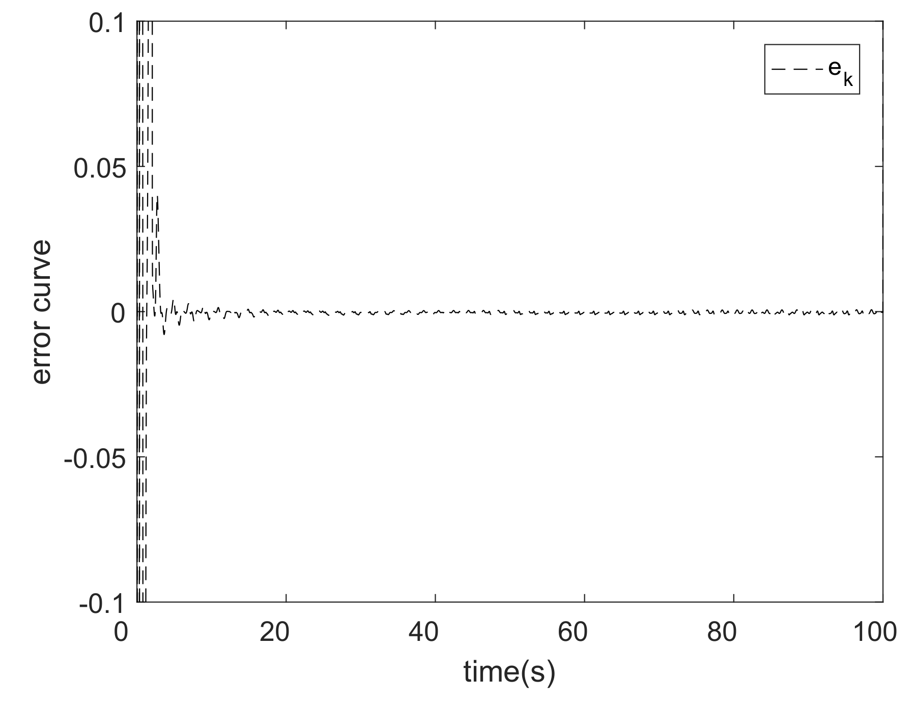
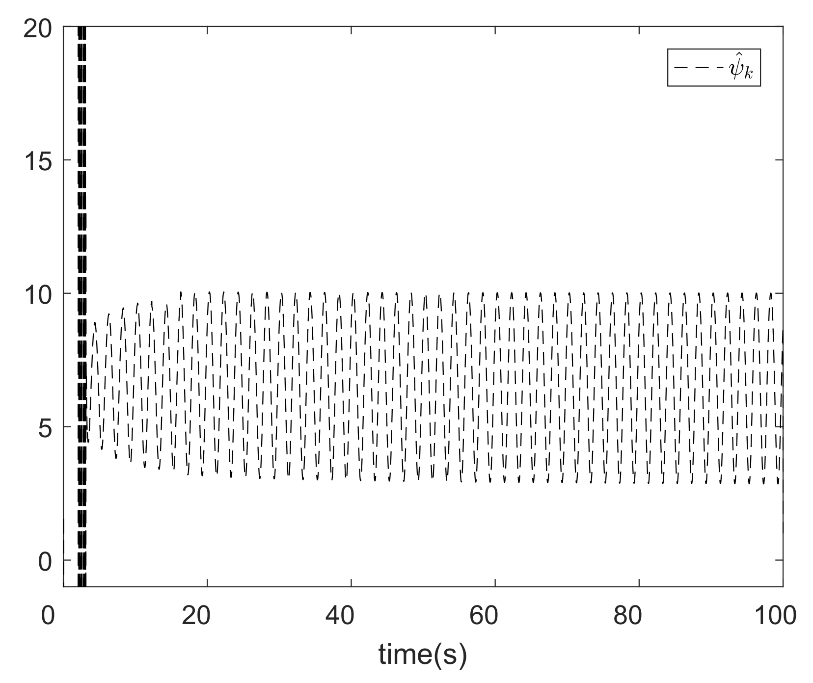
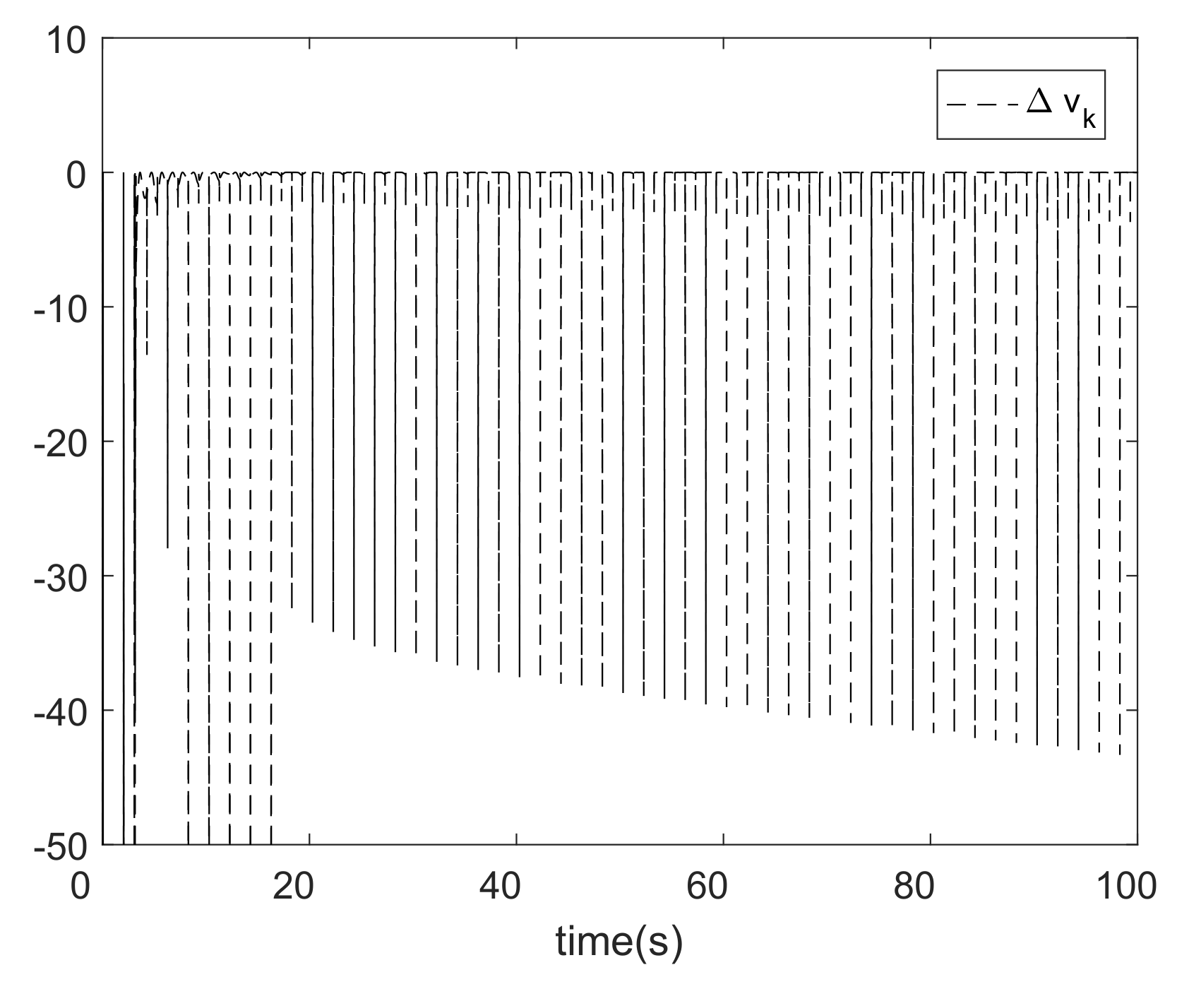
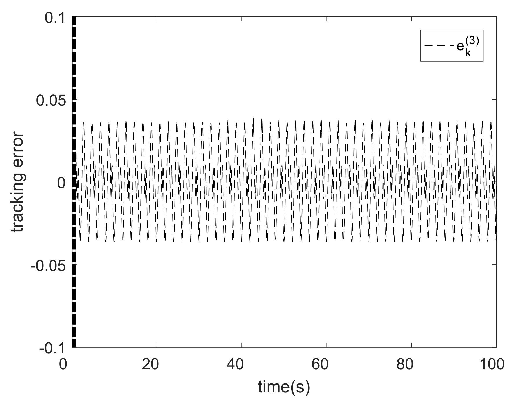
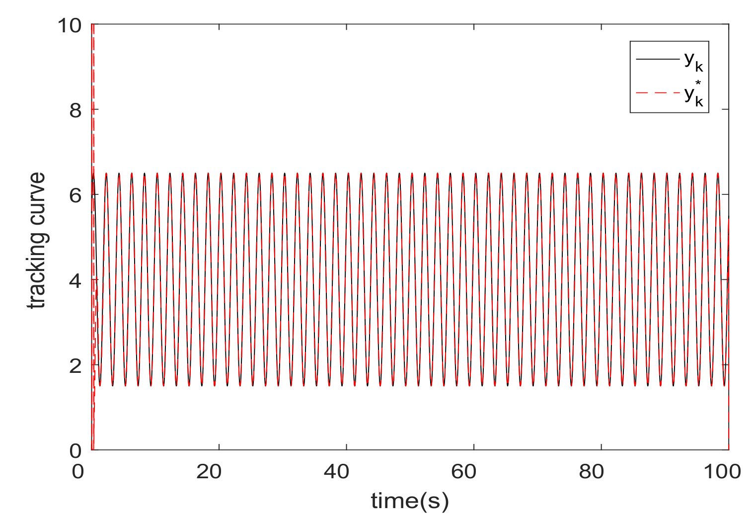
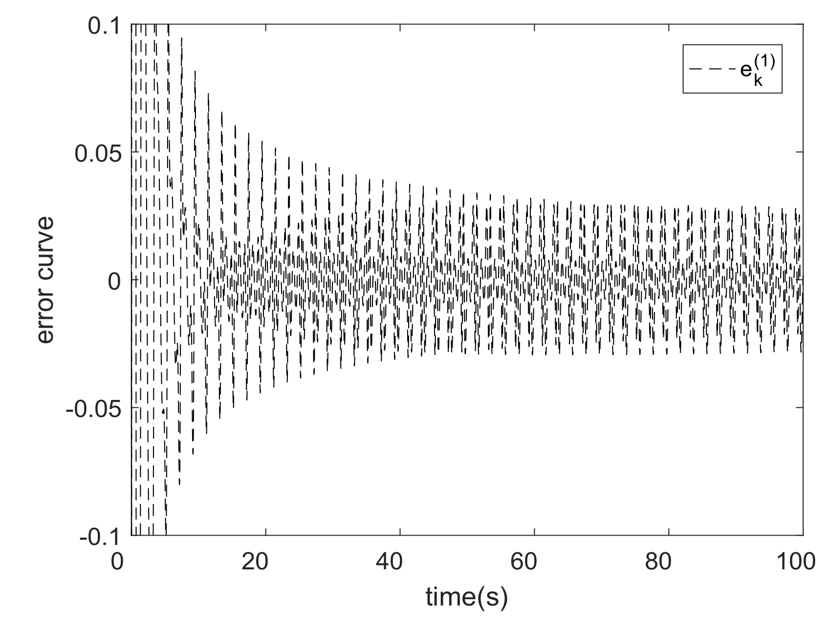
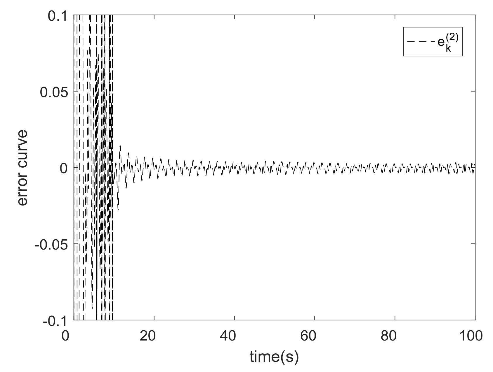
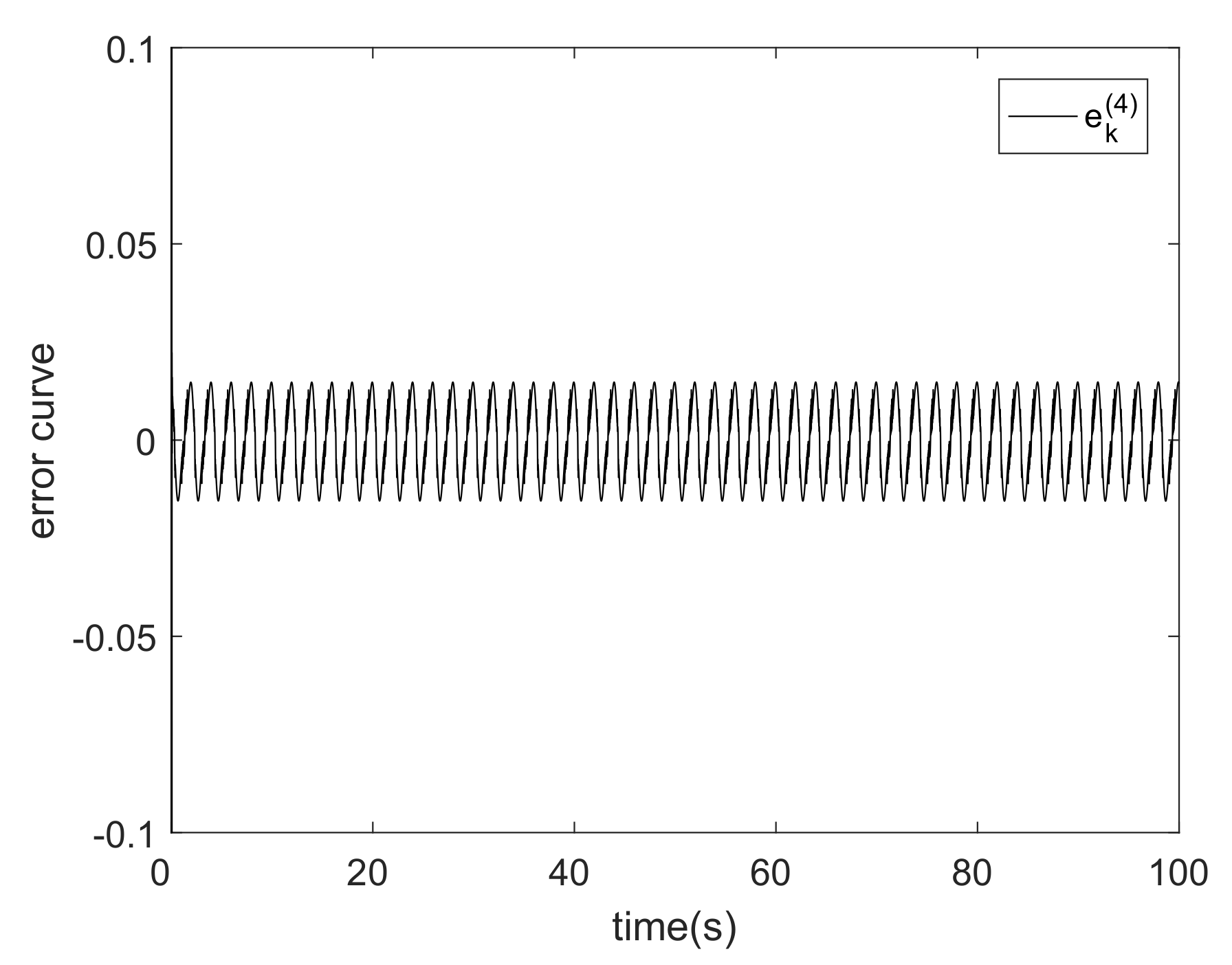
5. Analysis of Experimental Results

In this paper, EMREOS-ELM is investigated, and EMREOS-ELM is adopted for estimating the value ${\psi }_k$; EMREOS-ELM is an online learning algorithm and can train a single hidden layer neural network; besides it can adjust the network structure. In order to further show the effectiveness of the MFAC method based on EMREOS-ELM, the MFAC method based on another online learning algorithm is compared, and the online learning algorithm adjusts network structure using an incremental form. In order to describe this online learning algorithm easily, in this paper, this online learning algorithm is named as IREOS-ELM. The MFAC method based on IREOS-ELM also has three phases, parameter initialization, parameter learning and the adjustment of network structure. During the adjustment of network structure, all input weights and all hidden biases are reinitialized, and the network is retrained by using the $k-1$th training data. The MFAC method based on EMREOS-ELM is different from the MFAC method based on IREOS-ELM, it only initializes the input weight of the increased hidden node and the hidden bias of the increased hidden node, and it updates the output weights using the pseudoinverse of a partitioned matrix.

In this part, a simulation experiment is did, besides the MFAC algorithm based on EMREOS-ELM is compared with the MFAC algorithm based on RLS ([33] Equation 5.49), the MFAC method based on IREOS-ELM and RBF algorithm ([34] Equation 10.22).

In this numerical simulation experiment, the following single-input single-output unknown discrete-time nonlinear system is considered, and

$$y_{k+1}=\frac{y_k}{1+y_k^2}+u_k^3.$$

(55)

The discrete-time nonlinear system (55) comes from [35].

The reference signal is

$$y_{k+1}^{*}=4+2\sin (\pi T_{s}k)+1.5\cos (\pi T_{s}k)$$

(56)

where $T_s$ is the sampling time, and $T_s=0.01$.

The parameters of MFAC algorithm based on RLS are ${\rho }_k=1$, ${\lambda }_1=0.01$, and $a_0=0.95$. The activation function of EMREOS-ELM is sigmoid, $\lambda =0.1$, and $▵=0.002$. Figure 2, Figure 3, Figure 4, Figure 5 and Figure 6 show the main results of this numerical simulation experiment. Figure 2 plots the tracking curves, and in Figure 3, the curve denotes the tracking error change trend. Figure 4 shows the change trends of $E_k$ and $L_k$. Figure 4 indicates that the final value of $L_k$ is 9, when $L_k=9$, the tracking error satisfies $E_k\le E_m$, and the result of Figure 4 shows that EMEROS-ELM is effective in obtaining a compact network structure. Figure 5 indicates the change curve of ${\widehat{\psi }}_k$, ${\widehat{\psi }}_k={\mathit{H}}_k{\widehat{\mathit{\beta }}}_k$, and ${\widehat{\psi }}_k$ is the estimated value of ${\psi }_k$. In Section 4.4, the stability analysis of the MFAC algorithm based on EMREOS-ELM for unknown discrete-time nonlinear was stated, and we get the inequality (47). In order to verify the inequality (47), a new variable as

$$\Delta v_k\triangleq -{\sigma }_k({\gamma }_k^2{(e_{k+1}^{*})}^2-{▵}^2).$$

(57)

Figure 6 shows the change curve of of $\Delta v_k$, and it indicates that $\Delta v_k\le 0$.

Besides the error change curves of $e_k^{(1)}$, $e_k^{(2)}$, $e_k^{(3)}$ and $e_k^{(4)}$ are plotted in Figure 7, Figure 8, Figure 9 and Figure 10, respectively. Here $e_k^{(1)}$ indicates the error change curve of the REOS-ELM which has a fixed network structure, and the number of hidden nodes is 8; $e_k^{(2)}$ indicates the error change curve of the REOS-ELM which has a fixed network structure, and the number of hidden nodes is 20; $e_k^{(3)}$ is the error change curve of the MFAC algorithm based on RLS; and $e_k^{(4)}$ indicates the error change curve of RBF which has a fixed network structure, and the number of hidden nodes is 9. Figure 7, Figure 8, Figure 9 and Figure 10 indicate that the tracking effect of EMREOS-ELM is better than four other algorithms.

In order to further show the effectiveness of algorithms, the integral square error (ISE) index of predicted output is introduced, and

$$e_{\mathrm{ISE}}=\sum _{l=5000}^{10000}{(y_l^{*}-y_l)}^2.$$

(58)

Twenty groups of simulation experiments were done, and the ISE of those six control algorithms are shown in

Table 1. The simulation result $e_{\mathrm{ISE}}$.

	The MFAC Algorithm Based on REOS-ELM(L = 8)	The MFAC Algorithm Based on REOS-ELM(L = 20)	The MFAC Algorithm Based on EMREOS-ELM	RBFNN (L = 9)	The MFAC Algorithm Based on RLS	The MFAC Algorithm Based on IREOS-ELM
1	0.150672	0.002515	0.001562	0.550053	4.449964	0.012889
2	0.019459	0.040914	0.001705	0.502426	2.534129	0.433985
3	0.703282	0.014989	0.005451	0.564361	2.274406	0.016331
4	0.172610	0.150750	0.027222	0.504968	1.909120	0.017123
5	0.083149	0.244061	0.004806	0.402855	1.824217	0.007621
6	0.696841	0.009112	0.006475	0.411857	2.548398	0.004997
7	1.568039	0.051220	0.014730	0.591908	2.222298	0.182836
8	0.322919	0.024096	0.00295	0.584721	1.839572	0.009986
9	0.051606	0.576331	0.00295	0.524870	1.799829	0.048388
10	0.158293	0.678617	0.003559	0.696158	2.231448	0.001695
11	0.055251	0.004448	0.014255	0.551650	2.409947	0.015570
12	0.008733	0.004131	0.019071	0.493070	1.913370	0.046355
13	0.376944	0.008184	0.004649	0.553147	2.946602	0.012967
14	0.297452	0.01459	0.002863	0.633631	1.906357	0.054175
15	0.132094	0.329650	0.002116	0.730532	2.456959	0.016178
16	0.099835	0.194384	0.036917	0.779908	3.446312	0.017376
17	0.222907	0.002091	0.011495	0.431327	1.952456	0.049845
18	0.021288	0.002629	0.005704	0.561705	2.045576	0.049984
19	0.481443	0.004517	0.025093	0.582250	2.380352	0.007150
20	0.018625	0.212689	0.001724	0.664968	2.012102	0.016439
average value	0.282072	0.128496	0.009729	0.565818	2.354829	0.051094

. The final hidden node numbers of simulation experiments are showed in

Table 2. The final number of hidden nodes.

	1	2	3	4	5	6	7	8	9	10	11	12	13	14	15	16	17	18	19	20
The MFAC algorithm based on EMREOS-ELM	9	9	10	11	10	14	9	9	10	10	10	10	9	11	10	11	11	11	10	9
The MFAC algorithm based on IREOS-ELM	10	11	10	9	12	11	11	11	10	10	12	10	9	11	10	14	11	9	9	10

, and Table 2 shows that the MFAC method based on EMREOS-ELM is effective in adjusting network structure. The average values of ISE indicate that compared with five other control algorithms, the proposed algorithm has an improvement in the performance of control systems.

6. Conclusions

In order to analyse the stability of the MFAC algorithm based on REOS-ELM for unknown discrete-time nonlinear systems, an updating formula, which contains dead-zone characteristics, is introduced, and EMREOS-EM is investigated for the purpose of getting a more compact network structure and improving the performances of control systems. The proposed MFAC method based on EMREOS-ELM is compared with five other algorithms, and the simulation results show that the proposed algorithm has an improvement in the performance of control systems.

In this paper, the MFAC method based on EMREOS-ELM is introduced for single-input single-output unknown discrete-time nonlinear systems. In the future, we plan to do some work for multiple-input, multiple-output unknown discrete-time nonlinear systems based on the proposed algorithm, and in order to improve the performance of robot control systems, we will also apply this algorithm to robot control systems which are complex nonlinear systems.

References

1. Hou, Z.S.; Xu, J.X. On data-driven control theory: The state of the art and perspective. Acta Autom. Sin. 2009, 35, 650–667. [Google Scholar] [CrossRef]
2. Caponetto, R.; Dongola, G.; Fortuna, L.; Gallo, A. New results on the synthesis of FO-PID controllers. Commun. Nonlinear Sci. 2010, 15, 997–1007. [Google Scholar] [CrossRef]
3. Roman, R.C.; Precup, R.E.; David, R.C. Second order intelligent proportional-integral fuzzy control of twin rotor aerodynamic systems. Procedia Comput. Sci. 2018, 139, 372–380. [Google Scholar] [CrossRef]
4. Sanchez-Pena, R.S.; Colmegna, P.; Bianchi, F. Unfalsified control based on the controller parameterisation. Int. J. Syst. Sci. 2015, 46, 2820–2831. [Google Scholar] [CrossRef]
5. Safonov, M.G.; Tsao, T.C. The unfalsfied control concept and learning. IEEE Trans. Autom. Control 1997, 42, 2819–2824. [Google Scholar] [CrossRef]
6. Hou, Z.S.; Huang, W.H. The model-free learning adaptive control of a class of SISO nonlinear systems. In Proceedings of the 1997 American Control Conference, Albuquerque, NM, USA, 6 June 1997; Volume 1, pp. 343–344. [Google Scholar]
7. Hou, Z.S.; Jin, S.T. A novel data-driven control approach for a class of discrete-time nonlinear systems. IEEE Trans. Control Syst. Technol. 2011, 19, 1549–1558. [Google Scholar] [CrossRef]
8. Tutsoy, O.; Barkana, D.E.; Tugal, H. Design of a completely model free adaptive control in the presence of parametric, non-parametric uncertainties and random control signal delay. ISA Trans. 2018, 76, 67–77. [Google Scholar] [CrossRef]
9. Safaei, A.; Mahyuddin, M.N. Adaptive model-free control based on an ultra-local model with model-free parameter estimations for a generic SISO system. IEEE Access 2018, 6, 4266–4275. [Google Scholar] [CrossRef]
10. Hung-Yi, C.; Jin-Wei, L. Model-free adaptive sensing and control for a piezoelectrically actuated system. Sensors 2010, 10, 10545–10559. [Google Scholar]
11. Xia, Y.; Dai, Y.; Yan, W.; Xu, D.; Yang, C. Adaptive-observer-based data driven voltage control in islanded-mode of distributed energy resource systems. Energies 2018, 11, 3299. [Google Scholar] [CrossRef]
12. Hou, Z.S.; Xiong, S.S. On model free adaptive control and its stability analysis. IEEE Trans. Autom. Control 2019, in press. [Google Scholar] [CrossRef]
13. He, W.; Meng, T.T.; He, X.Y.; Samge, S.Z. Unified iterative learning control for flexible structures with input constraints. Automatica 2018, 96, 326–336. [Google Scholar] [CrossRef]
14. Xuan, Y.; Ruan, X. Reinforced gradient-type iterative learning control for discrete linear time-invariant systems with parameters uncertainties and external noises. IMA J. Math. Control Inf. 2016, 34, 1117–1133. [Google Scholar]
15. Miao, Y.; Wei, Z.; Liu, B.B. On iterative learning control for MIMO nonlinear systems in the presence of time-iteration-varying parameters. Nonlinear Dynam. 2017, 89, 2561–2571. [Google Scholar]
16. Hjalmarsson, H. Iterative feedback tuning—An overview. Int. J. Adapt. Control Signal Process. 2010, 16, 373–395. [Google Scholar] [CrossRef]
17. Heertjes, M.F.; Velden, B.V.D.; Oomen, T. Constrained iterative feedback tuning for robust control of a wafer stage system. IEEE Trans. Control Syst. Technol. 2016, 24, 56–66. [Google Scholar] [CrossRef]
18. RiosPatron, E.; Braatz, R. On the identification and control of dynamical systems using neural networks. IEEE Trans. Neural Netw. 1997, 8, 452. [Google Scholar]
19. Ren, X.M.; Lewis, F.L.; Zhang, J.L. Neural network compensation control for mechanical systems with disturbances. Automatic 2009, 45, 1221–1226. [Google Scholar] [CrossRef]
20. Wang, F.; Chen, B.; Lin, C.; Zhang, J.; Meng, X. Adaptive neural network finite-time output feedback control of quantized nonlinear systems. IEEE Trans. Cybern. 2018, 48, 1839–1848. [Google Scholar] [CrossRef]
21. Sun, C.Y.; He, W.; Ge, W.L.; Chang, C. Adaptive neural network control of biped robots. IEEE Trans. Syst. Man Cybern. Syst. 2017, 47, 315–326. [Google Scholar] [CrossRef]
22. Wang, M.S.; Tsai, T.M. Sliding mode and neural network control of sensorless PMSM controlled system for power consumption and performance improvement. Energies 2017, 10, 1780. [Google Scholar] [CrossRef]
23. Faria, J.; Pombo, J.; Calado, M.D.R.; Mariano, S. Power management control strategy based on artificial neural networks for standalone PV applications with a hybrid energy storage system. Energies 2019, 12, 902. [Google Scholar] [CrossRef]
24. Hou, Z.S.; Liu, S.D.; Tian, T.T. Lazy-learning-based data-driven model-free adaptive predictive control for a class of discrete-time nonlinear systems. IEEE Trans. Neural Netw. Learn. Syst. 2016, 28, 1–15. [Google Scholar] [CrossRef] [PubMed]
25. Zhu, Y.M.; Hou, Z.S. Data-driven MFAC for a class of discrete-time nonlinear systems with RBFNN. IEEE Trans. Neural Netw. Learn. Syst. 2014, 25, 1013–1020. [Google Scholar] [PubMed]
26. Huang, G.B.; Zhu, Q.Y.; Siew, C.K. Extreme learning machine: Theory and applications. Neurocomputing 2006, 70, 489–501. [Google Scholar] [CrossRef]
27. Liang, N.Y.; Huang, G.B.; Saratchandran, P.; Sundararajan, N. A fast and accurate online sequential learning algorithm for feedforward networks. IEEE Trans. Neural Netw. 2006, 17, 1411–1423. [Google Scholar] [CrossRef] [PubMed]
28. Jia, C.; Li, X.L.; Wang, K.; Ding, D.W. Adaptive control of nonlinear system using online error minimum neural networks. ISA Trans. 2016, 65, 125–132. [Google Scholar] [CrossRef] [PubMed]
29. Li, X.L.; Jia, C.; Liu, D.X.; Ding, D.W. Adaptive control of nonlinear discrete-time systems by using OS-ELM neural networks. Abstr. Appl. Anal. 2014, 2014, 1–11. [Google Scholar] [CrossRef]
30. Huynh, H.T.; Won, Y. Regularized online sequential learning algorithm for single-hidden layer feedforward neural networks. Pattern Recognit. Lett. 2011, 32, 1930–1935. [Google Scholar] [CrossRef]
31. Gao, X.H.; Wong, K.I.; Wong, P.K.; Chi, M.V. Adaptive control of rapidly time-varying discrete-time system using initial-training-free online extreme learning machine. Neurocomputing 2016, 194, 117–125. [Google Scholar] [CrossRef]
32. Huang, G.B.; Chen, L.; Siew, C.K. Universal approximation using incremental constructive feedforward networks with random hidden nodes. IEEE Trans. Neural Netw. 2006, 17, 879–892. [Google Scholar] [CrossRef] [PubMed]
33. Hong, Z.S. NonParametric Model and Adaptive Control Theory; Science Press: Beijing, China, 1999. [Google Scholar]
34. Kun, L.J. RBF Neural Network Adaptive Control Matlab Simulation; Tsinghua University Pre: Beijing, China, 2014. [Google Scholar]
35. Narendra, K.S. Identification and control for dynamic systems using neural networks using neural network. IEEE Trans. Inform. Theory 1990, 1, 4–27. [Google Scholar]
Figure 1. The process of the proposed MFAC method based on EMREOS-ELM.
Energies 12 03241 g001
Figure 2. The tracking curves of simulation experiment.
Energies 12 03241 g002
Figure 3. The changing trend of e k .
Energies 12 03241 g003
Figure 4. The changing trends of E k and L k .
Energies 12 03241 g004
Figure 5. The changing trend of ψ ^ k .
Energies 12 03241 g005
Figure 6. The changing trend of Δ v k .
Energies 12 03241 g006
Figure 7. The changing trend of e k ( 1 ) .
Energies 12 03241 g007
Figure 8. The changing trend of e k ( 2 ) .
Energies 12 03241 g008
Figure 9. The changing trend of e k ( 3 ) .
Energies 12 03241 g009
Figure 10. The changing trend of e k ( 4 ) .
Energies 12 03241 g010