Impact of Electrical Topology, Capacity Factor and Line Length on Economic Performance of Offshore Wind Investments


Abstract
1. Introduction
2. Description of Electrical Topologies Considered
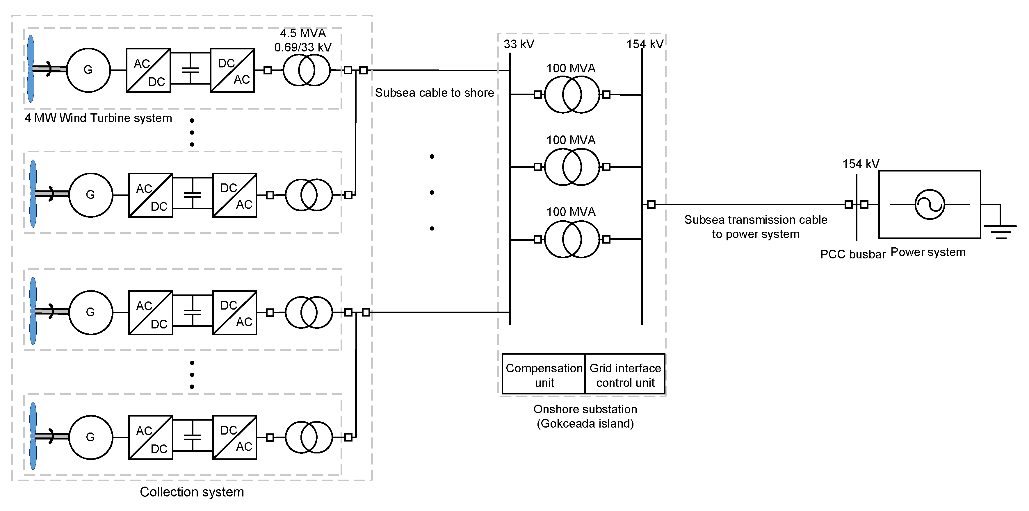
2.1. AC Offshore Wind Energy System
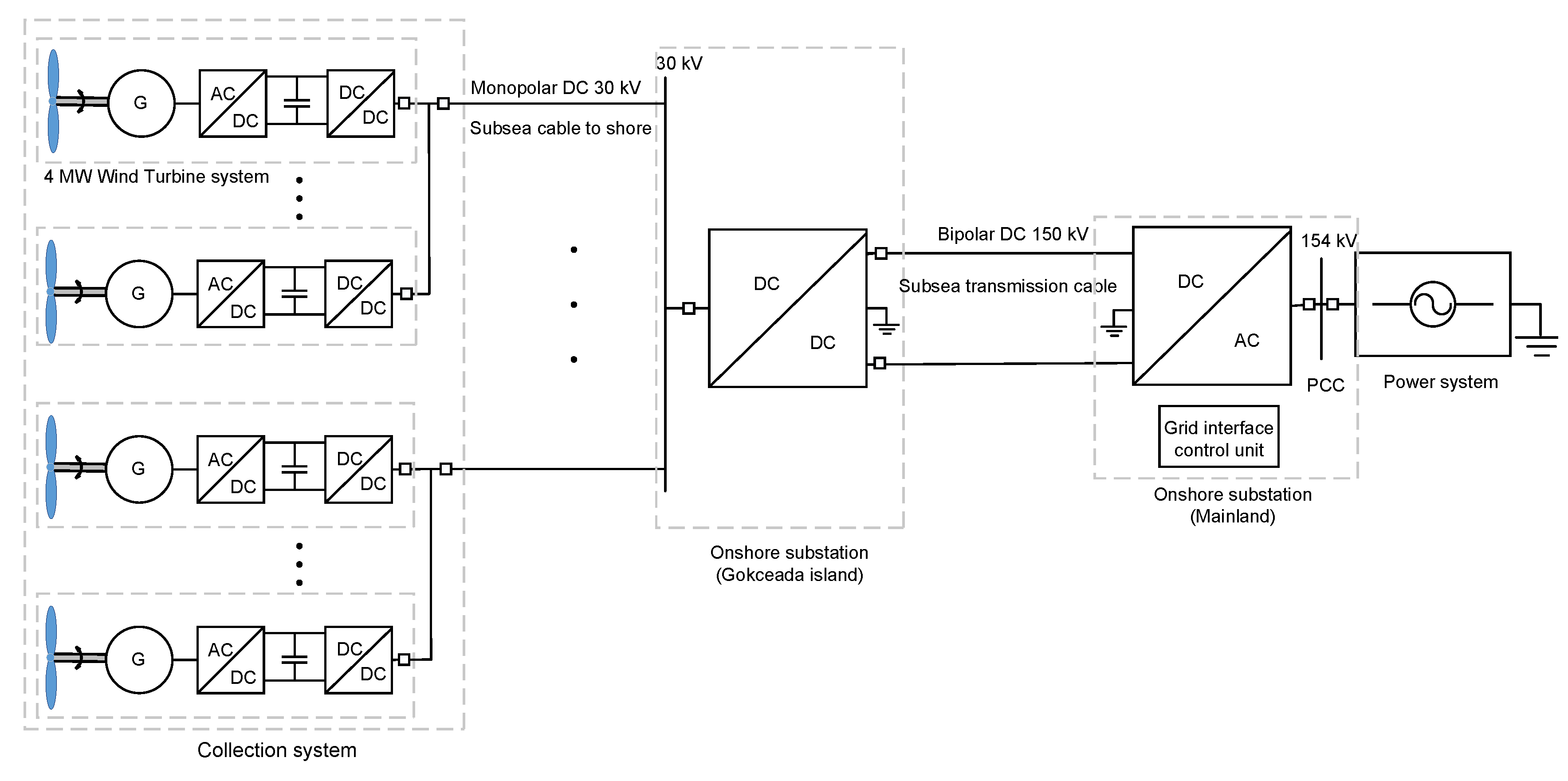
2.2. DC Offshore Wind Energy System
2.3. Electrical Design for Offshore Wind Farm Collection System
3. Annual Energy Yield and Electrical Losses Estimation
3.1. Power Electronics Losses
3.2. Transformer Losses
3.3. Collection and Transmission Lines Losses
3.4. Annual Energy Losses
4. Economic Analysis
4.1. Major Investment Indicators Considered For Economic Assessment
4.2. Cost Calculation for AC and DC Offshore Wind Energy Projects
4.3. CAPEX
4.3.1. Wind Turbine Cost
4.3.2. Support System Cost
4.3.3. Electrical System Cost
- Collection system cable cost—the wind turbines are connected to each other as well as to the onshore substation through submarine cables. The core (conductor) of the cables can be either stranded copper or aluminum. Due to the surrounding sea environment, sufficient electrical insulation is needed around the conductor. The subsea cable insulations are made of different dielectric materials. Among the two common ones are mass impregnated paper and Cross Linked Polyethylene (XLPE) Polymeric cables [42,43]. There are additional layers exist for shielding and mechanical strength purposes. For the DC configuration, XLPE cables are mostly used with VSC topology [44] and were therefore selected for this study. For the AC configuration, 3 core XLPE type cables were selected from available manufacturer datasheets. Reference [45] provides DC cable cost formulation for different voltages. Reference [25] presents a cost function for a 30 kV voltage level cable. The cost model used is given as follows [25]:where and are the cost constants of and 0.0068 for 30 kV, respectively. rated power of the cable [W]. The cost is converted to €/m and costs for different cross-sections of cables are calculated. The bipole 150 kV cable cost is calculated with the same formula with different constants ( and ) given in Reference [45]. The calculated cable costs in €/m are given in Table 2.Typical cable cross-sections were taken from a manufacturer’s [46] publicly available datasheet and depending on the selected voltage and power levels, cable costs are estimated as in Table 2. The cable cross sections were selected such that they carried the maximum power output of the wind turbines. It was considered that the selected radial collector system has a single cable in a row and carries the power of minimum 3 and maximum 13 wind turbine outputs in one feeder. These numbers were determined by considering the physical layout design as well as cable cross sections ampacity levels. An additional 40 m supplementary cable for each turbine was considered as recommended in Reference [38]. The total cable cost for DC collection system was calculated asThe cost function for 3 core XLPE cables given in Reference [39] was used to calculate the cable costs as follows:where , and are constants 52.08, 75.51 and 234.34, respectively. is the current ratings of the cables. Typical cable cross-sections with their current ratings were taken from two manufacturer’s available data sheets [47,48].The cables were considered to be buried under on the seabed. The burying cost in Reference [38] was used as 273 k€/km. The total burying cost for the collection system was calculated by considering all the cable lengths used in the system as
- Onshore DC/DC converter substation—one of the factors affecting the DC offshore wind system cost is converter costs. The percentage of the converters over the total cost varies based upon the system topology and transmission distance. Converter costs are found to be around 20% in References [49,50]. The DC configuration becomes more economical over the AC configuration once the converter cost is covered by the cable costs. In DC offshore wind systems, the onshore and offshore substations house the converters and a few other components such as reactors, filters and DC breakers. In addition, the offshore substations cost includes the platform cost as well. In this paper, since there were two onshore substations considered, platform cost was disregarded.Obtaining the exact cost figures for substation converter stations is very difficult. Reference [51] investigated many studies and proposed € 150/kW. Reference [45,52] presented 1 SEK/VA price for the converters. Reference [53] argues this is because of having different insulation levels at different voltages and proposes three different cost figures for different power ratings. Reference [52] states that this cost includes the cost of valves, filters and other necessary parts. The average of these figures given in the literature was used in this study, which is € 194.23/kVA by assuming that all the substation component costs are included. The onshore substation in the island is a DC/DC converter that steps up the voltage. It is assumed that the converter station includes a series connection of valves for the total power rating. The total price is calculated as
- Onshore AC substation and power factor correction costs—since the substation has many components including transformers, switchgeras, backup generators and so forth, the cost is considered as a lump sum that is a function of the installed wind power capacity. Based on the cost model in Reference [38], a cost of 50 k€/MW was used for the calculations. The cost models for power factor correction devices (i.e., SVC, STATCOM, shunt reactors) are given as follows [38]:Thus, the total substation cost is found [8] by
- Transmission line cost: The total power of 100 MW and 300 MW collected from wind turbines are delivered to onshore substation with the monopole collector system in DC collection system. The DC/DC converter in onshore substation steps up the collector voltage from 30 kV to 150 kV for HV transmission system. A bipole with two conductor system given in Reference [54] is considered for the transmission system from the onshore substation on the island to the other onshore substation on the mainland. The system has 150 kV voltage and two identical cables deliver the power as an underground (1.7 km) and subsea system (17.3 km). No overhead lines are considered for the transmission system. The two cables connecting the two substations share the total power due to being a bipole system and their cross-sections were considered based on the maximum current. The transmission cable cost that was calculated earlier was used for per km. Additional 100 km supplemental cable was considered and the total cable cost was calculated as:Since all the transmission cables are underground and subsea cables, a burying cost of 273 k€/km given in Equation (18) was used. In this study, close laying structure of cables was considered for the bipole system. The two cables were considered to be close to each other and buried together to have a single burying cost. The literature does not present any cost model for a single core XLPE cable used in the HVAC transmission system for high power delivery. It is also difficult to get the cost information from a manufacturer due to it being sensitive information for business operations. Therefore, it was assumed that a single core cable cost is 40% of the 3-core for the same current rating because of better insulation requirements for high voltage. The HVAC transmission system includes three single core cables, hence, the total cost for transmission system cable is tripled.
- Onshore DC/AC converter substation—the onshore substation on the mainland is a DC/AC substation that converts 150 kV DC to 154 kV AC national transmission voltage. Although this is a DC/AC converter, the price of € 194.23 /kVA used for the DC/DC converter in Equation (19) was used for the calculations. Many converters are connected together for the total power as considered earlier. Since the total cost is given as per power, the total cost considered with total power is in Equation (19).
- Grid connection cost—although the cost of the substation in the mainland was considered earlier, it was assumed that there is an additional grid connection cost at the point of common coupling in order to be connected to the 154 kV AC national electric transmission system. The cost for both AC and DC configuration is given as a function of total delivered power in Reference [38] as
4.3.4. Project Development, Management and Other Costs
4.4. OPEX
5. Results and Discussion
5.1. Losses Assessment
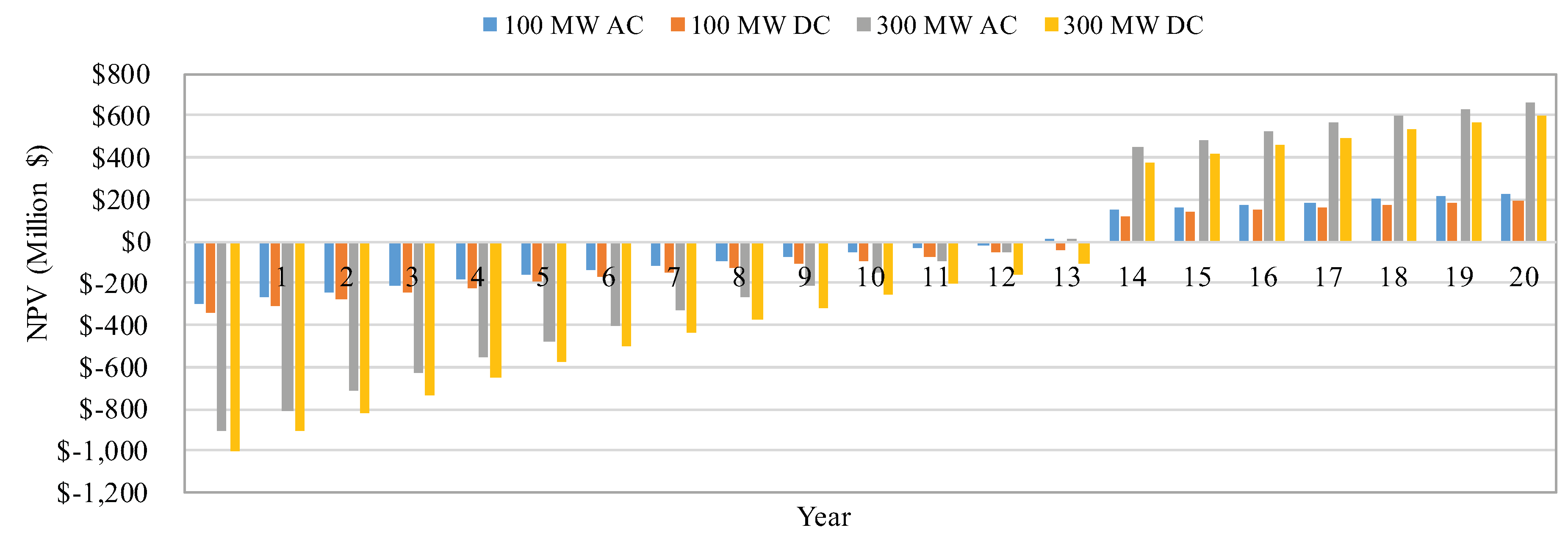
5.2. Economic Assessment
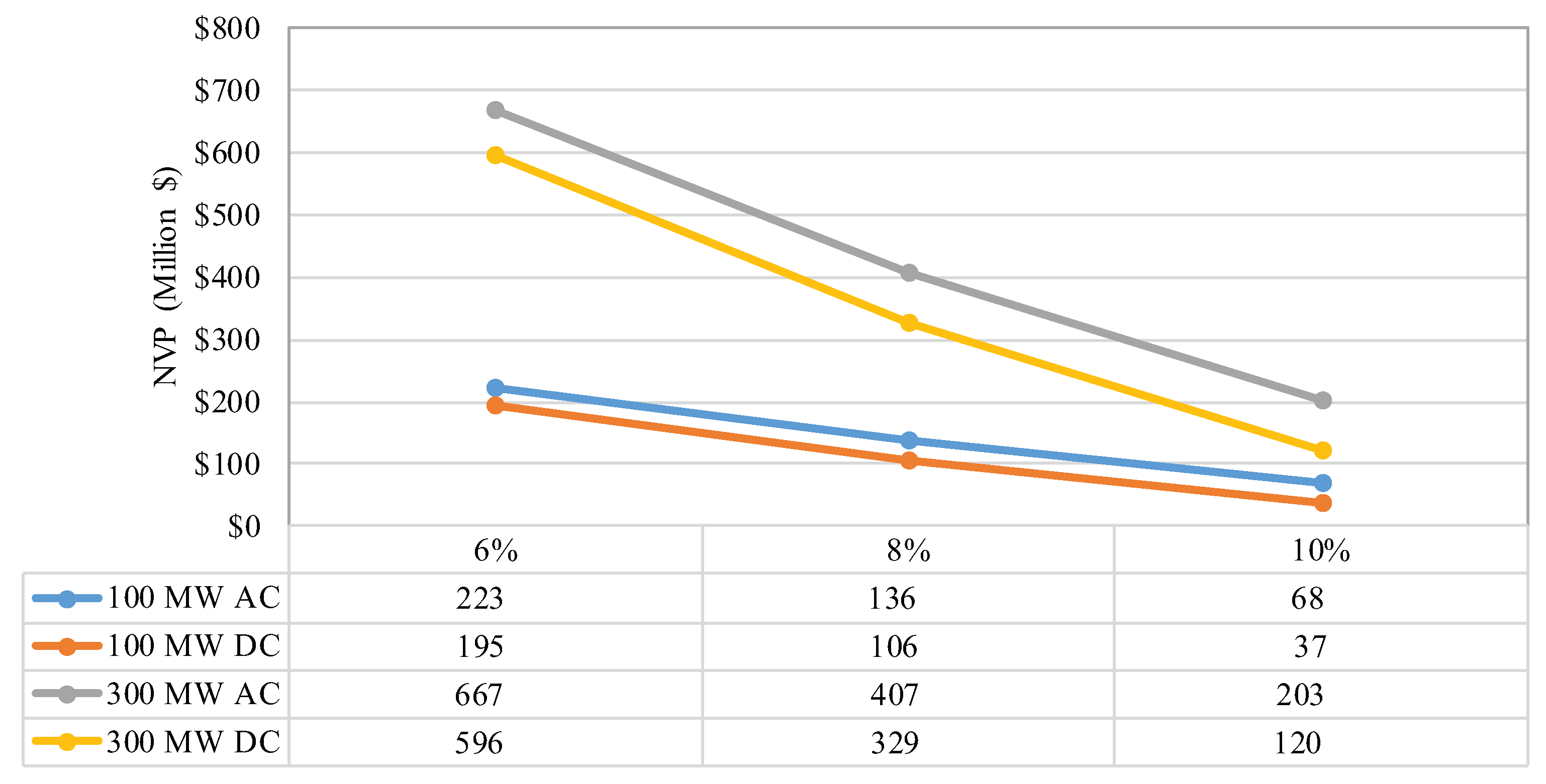
5.3. Sensitivity Analysis
6. Conclusions
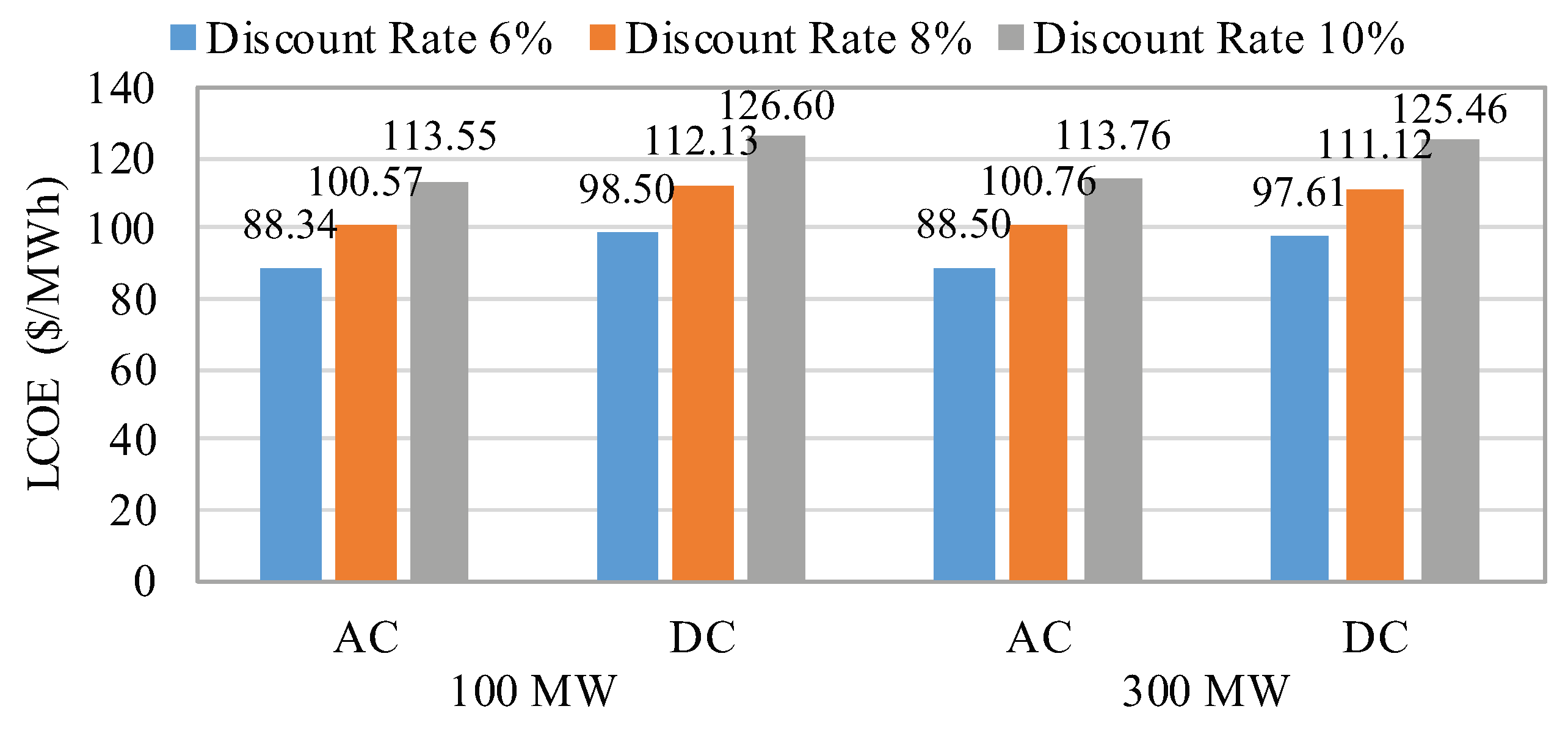
- The studied OWF was found to be economically viable for both AC and DC configurations with 13 and 14 years of DPBPs for the AC and DC options, respectively. The estimated LCOEs for the AC and DC OWF configurations range from 88.34 $/MWh to 113.76 $/MWh and from 97.61 $/MWh to 126.60 $/MWh, respectively. LCOEs for both options slightly change even though the wind farm size was increased by three-fold.
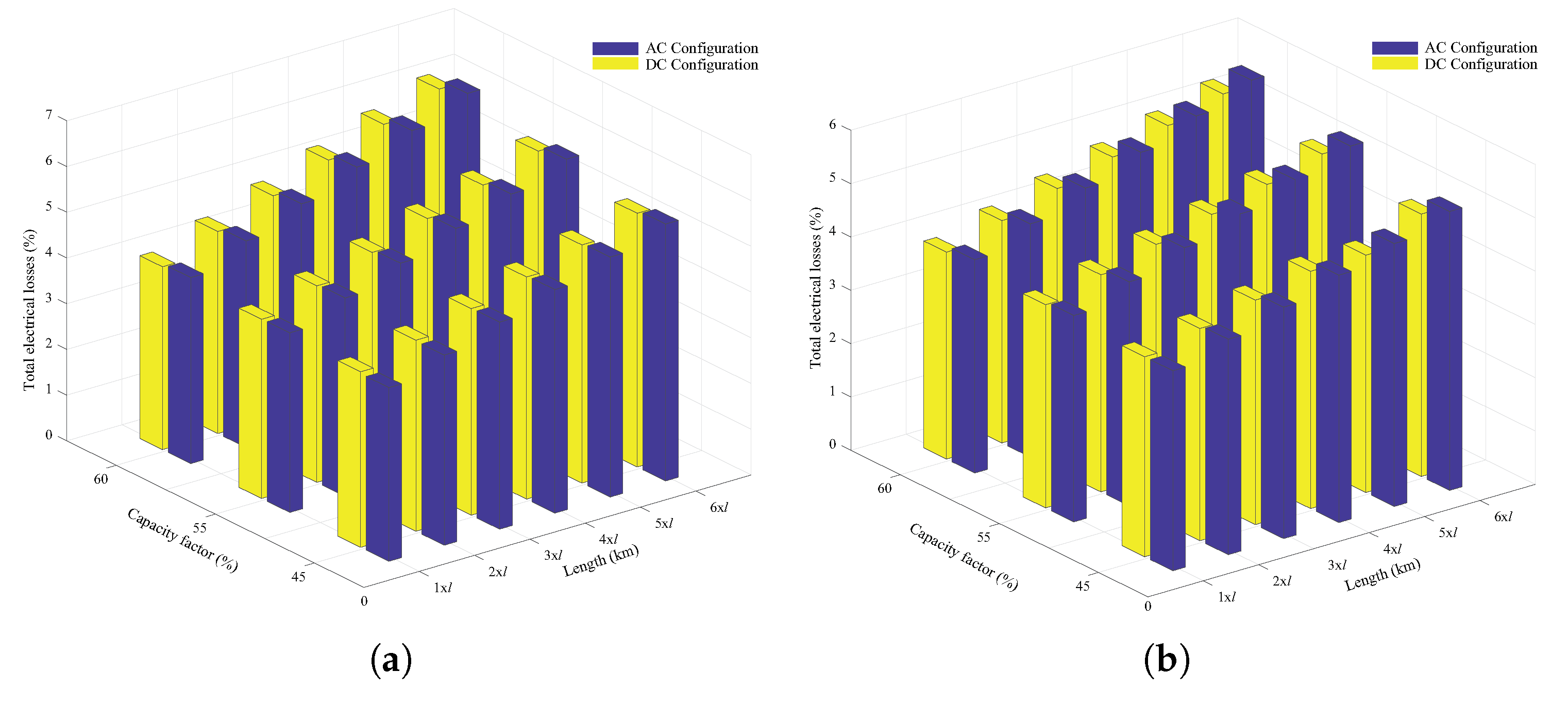
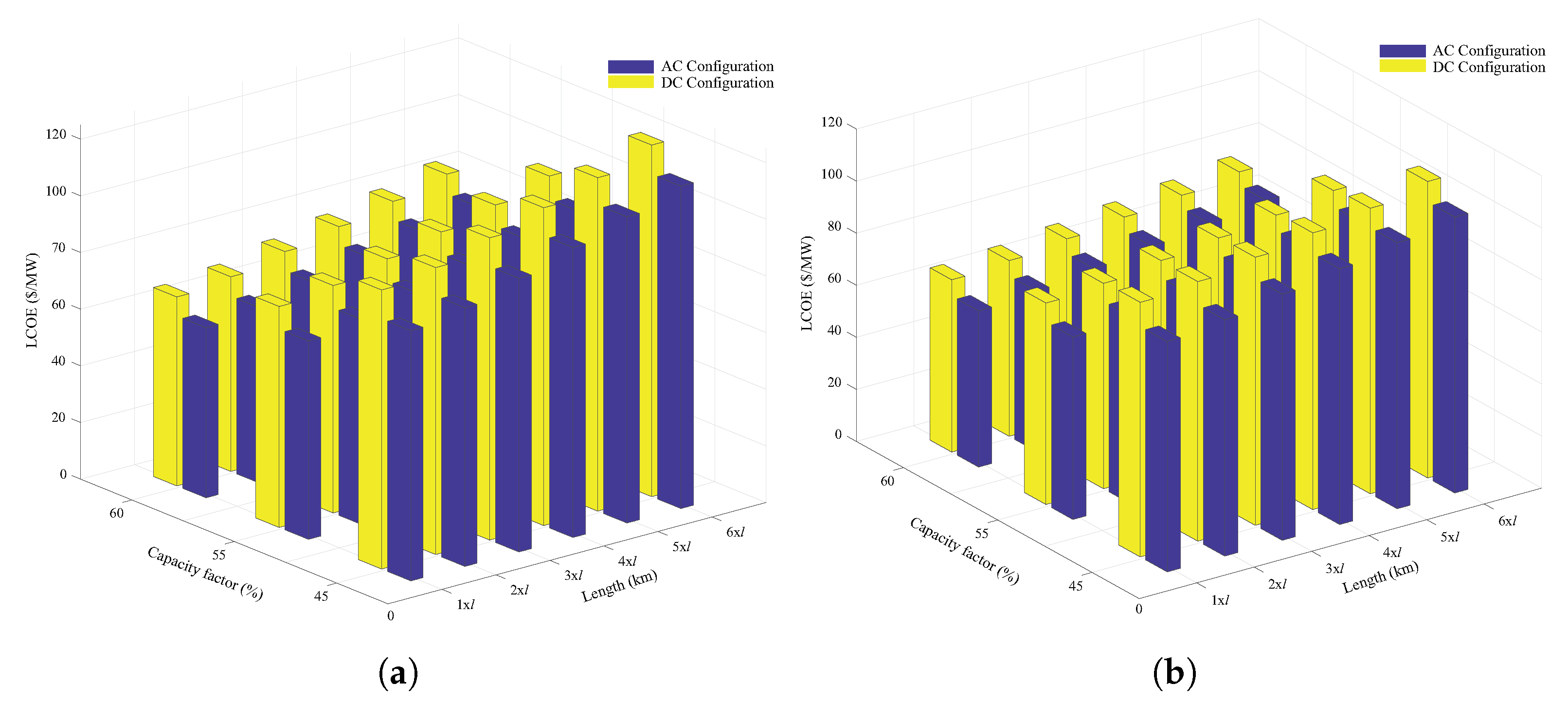
- Losses in the AC and DC configurations range from 3.75% to 5.86% and 3.75% to 5.34%, respectively, while LCOEs vary between 59.90 $/MWh and 113.76 $/MWh for the AC configuration and 66.21 $/MWh and 124.15 $/MWh for the DC configuration.
- It was found that the transmission line length parameter is more sensitive in loss estimation while the capacity factor parameter is more sensitive in LCOE estimation.
- It was proved that the superiority of AC configuration over the DC option in terms of LCOE decreases as capacity and transmission line length increase.
- It was also shown that the advantage of DC configuration over the AC option in terms of losses increased as capacity factor and transmission line length increased.
Author Contributions
Funding
Conflicts of Interest
References
- Enerdata. 2018 Global Energy Trends Report. Available online: http://www.enerdata.net (accessed on 28 May 2019).
- International Energy Agency (IEA). Available online: https://www.iea.org/geco/electricity/ (accessed on 10 August 2019).
- Saidur, R.; Islam, M.R.; Rahim, N.A.; Solangi, K.H. A review on global wind energy policy. Renew. Sustain. Energy Rev. 2010, 14, 1744–1762. [Google Scholar] [CrossRef]
- Argin, M.; Yerci, V.; Erdogan, N.; Kucuksari, S.; Cali, U. Exploring the offshore wind energy potential of Turkey based on multi-criteria site selection. Energy Strategy Rev. 2019, 23, 33–46. [Google Scholar] [CrossRef]
- Serrano Gonzalez, J.; Burgos Payan, M.; Riquelme Santos, J. Optimum design of transmissions systems for offshore wind farms including decision making under risk. Renew. Energy 2013, 59, 115–127. [Google Scholar] [CrossRef]
- Global Wind Energy Council (GWEC). Global Wind Report 2018. Available online: http://www.gwec.net (accessed on 30 April 2019).
- Salo, O.; Syri, S. What economic support is needed for Arctic offshore wind power? Renew. Sustain. Energy Rev. 2014, 31, 343–352. [Google Scholar] [CrossRef]
- Cali, U.; Erdogan, N.; Kucuksari, S.; Argin, M. Techno-economic analysis of high potential offshore wind farm locations in Turkey. Energy Strategy Rev. 2018, 22, 325–336. [Google Scholar] [CrossRef]
- Gardner, P. Offshore wind energy: Resources, technology and grid connection. In First International Workshop on Feasibility of HVDC Transmission for Offshore Wind Farms; KTH Royal Institute of Technology: Stockholm, Sweden, 2000. [Google Scholar]
- Houghton, T.; Bell, K.R.W.; Doquet, M. Offshore transmission for wind: Comparing the economic benefits of different offshore network configurations. Renew. Energy 2016, 94, 268–279. [Google Scholar] [CrossRef]
- Reed, G.F.; Hassan, H.A.A.; Korytowski, M.J.; Lewis, P.T.; Grainger, B.M. Comparison of HVAC and HVDC solutions for offshore wind farms with a procedure for system economic evaluation. In Proceedings of the IEEE Energytech, Cleveland, OH, USA, 21–23 May 2013; pp. 1–7. [Google Scholar]
- Morton, A.B.; Cowdroy, S.; Hill, J.R.A.; Halliday, M.; Nicholson, G.D. AC or DC? Economics of grid connection design for offshore wind farms. In Proceedings of the 8th IEE International Conference on AC and DC Power Transmission (ACDC 2006), London, UK, 28–31 March 2006; pp. 236–240. [Google Scholar]
- Ruddy, J.; Meere, R.; O’Donnell, T. Low Frequency AC transmission for offshore wind power: A review. Renew. Sustain. Energy Rev. 2016, 56, 75–86. [Google Scholar] [CrossRef]
- Gonzalez, J.S.; Payan, M.B.; Santos, J.M.R.; Gonzalez-Longatt, F. A review and recent developments in the optimal wind-turbine micro-siting problem. Renew. Sustain. Energy Rev. 2014, 30, 133–144. [Google Scholar] [CrossRef]
- Musasa, K.; Nwulu, N.I.; Gitau, M.N.; Bansal, R.C. Review on DC collection grids for offshore wind farms with high-voltage DC transmission system. IET Power Electron. 2017, 10, 2104–2115. [Google Scholar] [CrossRef]
- Gil, M.D.P.; Domínguez-García, J.L.; Díaz-González, F.; Aragüés-Peñalba, M.; Gomis-Bellmunt, O. Feasibility analysis of offshore wind power plants with DC collection grid. Renew. Energy 2015, 78, 467–477. [Google Scholar]
- Xu, L.; Yao, L. DC voltage control and power dispatch of a multi-terminal HVDC system for integrating large offshore wind farms. IET Renew. Power Gener. 2011, 5, 223–233. [Google Scholar] [CrossRef]
- Kong, X.; Jia, H. Techno-Economic Analysis of SVC-HVDC Transmission System for Offshore Wind. In Proceedings of the 2011 Asia-Pacific Power and Energy Engineering Conference, Wuhan, China, 25–28 March 2011; pp. 1–5. [Google Scholar]
- Xiang, X.; Merlin, M.M.C.; Green, T.C. Techno-Cost analysis and comparison of HVAC, LFAC and HVDC for offshore wind power connection. In Proceedings of the 12th IET International Conference on AC and DC Power Transmission (ACDC 2016), Beijing, China, 28–29 May 2016. [Google Scholar]
- Hassan, A. Hamdan and Brian Kinsella. Using a VSC Based HVDC Application to Energize Offshore Platforms from Onshore—A Life-cycle Economic Appraisal. Energy Procedia 2017, 105, 3101–3111. [Google Scholar]
- Eeckhout, B.V. The Economic Value of VSC HVDC Compared to HVAC for Offshore Wind Farms. Ph.D. Thesis, Katholieke Universiteit Leuven, Leuven, Belgium, 2007. [Google Scholar]
- Elliott, D.; Bell, K.R.W.; Finney, S.J.; Adapa, R.; Brozio, C.; Yu, J.; Hussain, K. A Comparison of AC and HVDC Options for the Connection of Offshore Wind Generation in Great Britain. IEEE Trans. Power Deliv. 2016, 31, 798–809. [Google Scholar] [CrossRef]
- Abdulrahman, A.; Santiago, B.; Omar, E.; Grain, A.; Callum, M. HVDC Transmission: Technology Review, Market Trends and Future Outlook. Renew. Sustain. Energy Rev. 2019, 112, 530–554. [Google Scholar]
- Johnson, M.H.; Aliprantis, D.C.; Chen, H. Offshore wind farm with DC collection system. In Proceedings of the 2013 IEEE Power and Energy Conference at Illinois (PECI), Champaign, IL, USA, 22 February 2013; pp. 53–59. [Google Scholar]
- Lakshmanan, P.; Liang, J.; Jenkins, N. Assessment of collection systems for HVDC connected offshore wind farms. Electr. Power Syst. Res. 2015, 129, 75–82. [Google Scholar] [CrossRef]
- Ebenhoch, R. Comparative Levelized Cost of Energy Analysis. Energy Procedia 2015, 80, 108–122. [Google Scholar] [CrossRef]
- Masters, G.M. Renewable and Efficient Electric Power Systems; John Wiley & Sons: Hoboken, NJ, USA, 2013. [Google Scholar]
- Cali, U. Grid and Market Integration of Large-Scale Wind Farms Using Advanced Wind Power Forecasting: Technical and Energy Economic Aspects; Kassel University Press GmbH: Kassel, Germany, 2011; pp. 1–156. [Google Scholar]
- Renewables.ninja. 2017. Available online: https://www.renewables.ninja/ (accessed on 29 January 2019).
- Staffell, I.; Pfenninger, S. Using bias-corrected reanalysis to simulate current and future wind power output. Energy 2016, 114, 1224–1239. [Google Scholar] [CrossRef]
- Siemens. Wind Turbine SWT-4.0-130 Technical Specifications. 2015. Available online: https://www.thewindpower.net/scripts/fpdf181/turbine.php?id=957 (accessed on 25 May 2019).
- Al Ameri, A.; Ounissa, A.; Nichita, C.; Djamal, A. Power Loss Analysis for Wind Power Grid Integration Based on Weibull Distribution. Energies 2017, 10, 463. [Google Scholar] [CrossRef]
- ABB. HiPak IGBT Modules Data Sheet. 2014. Available online: www.abb.com/semiconductors (accessed on 12 January 2019).
- Zhang, X.; Green, T.C. The modular multilevel converter for high step-up ratio DC–DC conversion. IEEE Trans. Ind. Electron. 2015, 62, 4925–4936. [Google Scholar] [CrossRef]
- Gultekin, B.; Gercek, C.O.; Atalik, T.; Deniz, M.; Bicer, N.; Ermis, M.; Kose, K.N.; Ermis, C.; Ko, E.; Cadirci, I.; et al. Design and Implementation of a 154-kV±50-Mvar Transmission STATCOM Based on 21-Level Cascaded Multilevel Converter. IEEE Trans. Ind. Appl. 2012, 48, 1030–1045. [Google Scholar] [CrossRef]
- Mamane, C. Transformer Loss Evaluation: User-Manufacturer Communications. IEEE Trans. Ind. Appl. 1984, 20, 11–15. [Google Scholar] [CrossRef]
- Lerch, M.; De-Prada-Gil, M.; Molins, C.; Benveniste, G. Sensitivity analysis on the levelized cost of energy for floating offshore wind farms. Sustain. Energy Technol. Assess. 2018, 30, 77–90. [Google Scholar] [CrossRef]
- Gonzalez-Rodrigue, A.G. Review of offshore wind farm cost components. Energy Sustain. Dev. 2017, 37, 10–19. [Google Scholar] [CrossRef]
- Dicorato, M.; Forte, G.; Pisani, M.; Trovato, M. Guidelines for assessment of investment cost for offshore wind generation. Renew. Energy 2011, 36, 2043–2051. [Google Scholar] [CrossRef]
- Wei, Q.; Wu, B.; Xu, D.; Zargari, N.R. IOP Conference Series: Earth and Environmental Science. In Proceedings of the 12th IET International Conference on AC and DC Power Transmission (ACDC 2016), Beijing, China, 28–29 May 2016. [Google Scholar]
- Koch, H.; Retzmann, D. Connecting large offshore wind farms to the transmission network. In Proceedings of the IEEE PES T&D 2010, New Orleans, LA, USA, 19–22 April 2010. [Google Scholar]
- Europa Cable. An Introduction to High Voltage Direct Current (HVDC) Underground Cables. Technical Brochure. Available online: www.europacable.eu (accessed on 12 January 2019).
- ENSO. Offshore Transmission Technology. 2011. Available online: https://www.entsoe.eu (accessed on 20 February 2019).
- Zaccone, E. High voltage underground and subsea cable technology options for future transmission in Europe. In Proceedings of the European Electricity Grid Initiative E-Highway 2050 Workshop, Brussels, Belgium, 15 April 2014. [Google Scholar]
- Lundberg, S. Performance Comparison of Wind Park Configurations; Technical Report; Chalmers University of Technology: Gothenburg, Sweden, 2003. [Google Scholar]
- ABB. HVDC Light. 2011. Available online: www.new.abb.com/docs/default-source/ewea-doc/hvdc-light.pdf (accessed on 20 February 2019).
- BS6622/BS7835 Three Core Armoured 33kV XLPE Stranded Copper Conductors. Prysmian. 2011. Available online: www.powerandcables.com (accessed on 20 February 2019).
- BS6622/BS7835 Three Core Armoured 33kV XLPE Stranded Copper Conductors. 6-36kV Medium Voltage Underground Power Cables XLPE Insulated Cables. 2019. Available online: www.nexans.co.uk (accessed on 20 February 2019).
- Nieradzinska, K.; MacIver, C.; Gill, S.; Agnew, G.A.; Anaya-Lara, O.; Bell, K.R.W. Optioneering analysis for connecting Dogger Bank offshore wind farms to the GB electricity network. Renew. Energy 2016, 91, 120–129. [Google Scholar] [CrossRef]
- Daniel Manrique, O. Design of the HVDC Connection of a 425 MW Offshore Wind Farm to the German Network; Technical Report; Universidad Pontificia: Madrid, Spain, 2017. [Google Scholar]
- Stamatiou, G. Techno-Economical Analysis of DC Collection Grid for Offshore Wind Parks. Master’s Thesis, The University of Nottingham, Nottingham, UK, 2010. [Google Scholar]
- Lazaridis, L.P. Economic Comparison of HVAC and HVDC Solutions for Large Offshore Wind Farms underSpecial Consideration of Reliability. Master’s Thesis, School of Electrical Engineering, KTH, Stockholm, Sweden, 2005. [Google Scholar]
- Stamatiou, G.; Srivastava, K.; Reza, M.; Zanchetta, P. Economics of DC Wind Collection Grid as Affected by Cost of Key Components. In Proceedings of the World Renewable Energy Congress-Sweden, Linköping, Sweden, 8–13 May 2011. [Google Scholar]
- Korompili, A.; Wu, Q.; Zhao, H. Review of VSC HVDC connection for offshore wind power integration. Renew. Sustain. Energy Rev. 2016, 59, 1405–1414. [Google Scholar] [CrossRef]
- Heimiller, D.; Ho, J.; Moné, C.; Hand, M. 2015 Cost of Wind Energy Review. In National Renewable Energy Laboratory/TP-6A20-66861 Technical Report; 2017; 115p. Available online: https://www.nrel.gov/docs/fy17osti/66861.pdf (accessed on 12 July 2019).
- Kempton, W.; McClellan, S.; Ozkan, D. Massachusetts offshore wind future cost study. Special Initiative on Offshore Wind; University of Delaware: Newark, DE, USA, 2016. [Google Scholar]
- Kim, J.-Y.; Oh, K.-Y.; Kang, K.-S.; Lee, J.-S. Site selection of offshore wind farms around the korean peninsula through economic evaluation. Renew. Energy 2013, 54, 189–195. [Google Scholar] [CrossRef]


| Parameter | 5SNA 3600E170300 | 5SNA 1200G450300 | 5SNA 0750G650300 |
|---|---|---|---|
| (V) | 1700 | 4500 | 6500 |
| (A) | 3600 | 1200 | 750 |
| (V) | 2.5 | 2.6 | 2.9 |
| (m) | 0.055 | 0.07 | 0.07 |
| (mJ) | 1100 | 4350 | 6400 |
| (mJ) | 1600 | 6000 | 5300 |
| (V) | 1.85 | 3.2 | 3.2 |
| (m) | 0.094 | 0.34 | 0.13 |
| (mJ) | 1080 | 2730 | 2700 |
| Voltage (kV) | Topology | Cable Cross-Section (mm) | Price (€/m) |
|---|---|---|---|
| 30 | Monopole | 95 | 50 |
| 30 | Monopole | 120 | 61 |
| 30 | Monopole | 185 | 86 |
| 30 | Monopole | 300 | 124 |
| 30 | Monopole | 400 | 147 |
| 30 | Monopole | 500 | 175 |
| 30 | Monopole | 630 | 207 |
| 30 | Monopole | 1000 | 279 |
| 30 | Monopole | 1400 | 339 |
| 30 | Monopole | 1600 | 368 |
| 150 | Bipole | 150 | 201 |
| 150 | Bipole | 630 | 479 |
| AC Configuration | 100 MW | 300 MW | ||
| (kWh) | (%) | (kWh) | (%) | |
| Collection cables | 190,564 | 0.05 | 700,393 | 0.06 |
| Transmission cable | 1,422,127 | 0.36 | 3,490,676 | 0.30 |
| Total line losses | 1,612,692 | 0.41 | 4,191,070 | 0.36 |
| Power electronics including transformer | 13,256,069 | 3.39 | 39,768,206 | 3,39 |
| Total energy losses | 14,868,760 | 3.80 | 43,959,276 | 3,75 |
| DC Configuration | 100 MW | 300 MW | ||
| (kWh) | (%) | (kWh) | (%) | |
| Collection cables | 129,018 | 0.03 | 515,944 | 0.04 |
| Transmission cable | 1,069,279 | 0.27 | 2,748,187 | 0.23 |
| Total line losses | 1,198,297 | 0.31 | 3,264,131 | 0.28 |
| Power electronics | 13,552,123 | 3.46 | 40,697,999 | 3.47 |
| Total energy losses | 14,750,420 | 3.77 | 43,962,129 | 3.75 |
| AC 100 MW | DC 100 MW | AC 300 MW | DC 300 MW | |
|---|---|---|---|---|
| Capacity factor at PCC (%) | 41.24 | 41.20 | 41.24 | 41.24 |
| Net AEP (kWh/year) | 361,344,935 | 361,194,688 | 1,084,598,234 | 1,084,598,234 |
| Annual Revenue with base FIT (million$) | 26.38 | 26.37 | 79,18 | 79,18 |
| Annual Revenue with max FIT (million$) | 39.75 | 39.73 | 119.31 | 119.31 |
| CAPEX (million$) | 300.59 | 335.01 | 903.88 | 998.72 |
| OPEX (million$/20 years) | 5.71 | 6.37 | 17.17 | 18.98 |
© 2019 by the authors. Licensee MDPI, Basel, Switzerland. This article is an open access article distributed under the terms and conditions of the Creative Commons Attribution (CC BY) license (http://creativecommons.org/licenses/by/4.0/).
Share and Cite
Kucuksari, S.; Erdogan, N.; Cali, U. Impact of Electrical Topology, Capacity Factor and Line Length on Economic Performance of Offshore Wind Investments. Energies 2019, 12, 3191. https://doi.org/10.3390/en12163191
Kucuksari S, Erdogan N, Cali U. Impact of Electrical Topology, Capacity Factor and Line Length on Economic Performance of Offshore Wind Investments. Energies. 2019; 12(16):3191. https://doi.org/10.3390/en12163191
Chicago/Turabian StyleKucuksari, Sadik, Nuh Erdogan, and Umit Cali. 2019. "Impact of Electrical Topology, Capacity Factor and Line Length on Economic Performance of Offshore Wind Investments" Energies 12, no. 16: 3191. https://doi.org/10.3390/en12163191
APA StyleKucuksari, S., Erdogan, N., & Cali, U. (2019). Impact of Electrical Topology, Capacity Factor and Line Length on Economic Performance of Offshore Wind Investments. Energies, 12(16), 3191. https://doi.org/10.3390/en12163191