Proton Exchange Membrane Fuel Cell Stack Design Optimization Using an Improved Jaya Algorithm

Abstract

Fuel cell stack configuration optimization is known to be a problem that, in addition to presenting engineering challenges, is computationally hard. This paper presents an improved computational heuristic for solving the problem. The problem addressed in this paper is one of constrained optimization, where the goal is to seek optimal (or near-optimal) values of (i) the number of proton exchange membrane fuel cells (PEMFCs) to be connected in series to form a group, (ii) the number of such groups to be connected in parallel, and (iii) the cell area, such that the PEMFC assembly delivers the rated voltage at the rated power while the cost of building the assembly is as low as possible. Simulation results show that the proposed method outperforms four of the best-known methods in the literature. The improvement in performance afforded by the proposed algorithm is validated with statistical tests of significance.

1. Introduction

Energy has been identified as “humanity’s number one problem for the next 50 years” [1]. Fuel cells [2,3,4,5,6], which are electrochemical devices that convert chemical energy to electrical energy, offer a viable alternative to fossil-fuel-based sources of energy. Of the various types of fuel cells (see, for example, references [6,7] for an overview), proton exchange membrane (or polymer electrolyte membrane) fuel cells, or PEMFCs, provide a relatively low-cost, low-temperature, high-efficiency and near-zero-pollution energy source for both stationary and portable applications. This paper uses a machine learning approach to address a PEM fuel cell problem of practical interest.

Fuel cells are complex systems whose electrochemistry, thermodynamics and engineering have not yet been fully understood. The complexity and non-linearity of the underlying processes in fuel cells (and many other areas of energy research) are often too hard for physics-, chemistry-, or engineering-based methods to build and interpret models that offer a balance between theoretical rigor and practical usefulness. It is here that data-driven or machine learning approaches come in handy, providing an alternative route to predictive analysis and parameter optimization.

The literature on the use of machine learning in energy research is vast; a few representative examples are mentioned below. A recent example of the use of deep learning (e.g., [8]) in nuclear fusion energy is found in [9] where a method has been developed for predicting disruptive instabilities in controlled fusion plasmas in magnetic-confinement tokamak reactors. Related work on the same type of problem has used machine learning strategies such as neural network [10,11,12], fuzzy logic and regression trees [13], support vector machine classification [14], and genetic algorithms [15]. Deep neural network is shown to outperform linear regression and (shallow) neural network for a short-term natural gas load forecasting application [16]. A problem of allocating optical links for connecting automatic circuit breakers in a utility power grid has been solved using a multi-objective genetic algorithm (NSGA-II) [17] in [18]. Energy optimization under performance constraints in chip multiprocessor systems has been addressed in [19] where deep neural network is shown to outperform reinforcement learning (e.g., [20]) and Kalman filtering (e.g., [21]). Training a neural network on weather and turbine data, Google’s DeepMind system predicted “wind power output 36 hours ahead of actual generation … [and] boosted the value of … wind energy by roughly 20 percent” [22]. A study of the prediction of hydrogen production via biomass gasification is undertaken in [23] where the following four algorithms (e.g., [24,25]) are used: linear regression, K-nearest neighbors regression, support vector machine regression, and decision tree regression.

Modeling, simulation, design, development and control of fuel cells and fuel cell-based systems present a variety of challenges, some of which have, in recent years, been formulated as classification, clustering, regression or optimization and addressed with computational (algorithmic) approaches based on machine learning. Examples abound; just a few illustrative ones are mentioned here. Genetic programming (e.g., [26,27]) is used in a supervised learning mode for static and dynamic (load-following) modeling of solid oxide fuel cells (SOFCs) [28] and also in the optimization of the forming process of bipolar plates of PEMFCs [29]. Differential evolution (e.g., [30,31]) is used to optimize seven parameters for modeling the polarization curve of a PEMFC stack [32]. An adaptive-neuro-fuzzy-inference-system-based maximum-power-point-tracking controller is designed [33] for a proton exchange membrane fuel cell system used in electric vehicle applications. Fault classification of PEMFCs that are used in trams is achieved by employing a hidden Markov model (HMM) approach (e.g., [25]) in [34] where K-means clustering (e.g., [24]) is used to eliminate singular data points as part of the preprocessing step before the HMM is applied; classification results produced by the HMM are shown to be better than those produced by the support vector machine method. Deep learning is applied [35] to sequence fault diagnosis of a PEMFC water management subsystem. Particle swarm optimization [36] is used in component sizing for a PEMFC-battery hybrid system for locomotive applications [37]. Adaptive neuro-fuzzy controllers are designed [38] for performance enhancement of PEMFCs. A prediction method for PEMFC performance degradation is proposed [39] using long short-term memory (LSTM) recurrent neural network [40] along with the auto-regressive integrated moving average (ARIMA) method.

In practical applications, for meeting specific output voltage, current or power requirements, a number of fuel cells are typically assembled in series and/or parallel connections. The design of the stack configuration of fuel cells for use as stand-alone power-supply systems presents engineering challenges and is a non-trivial computational problem (e.g., [41,42,43]). This paper addresses the design problem considered in [41,42,43]. Specifically, the problem is to find optimal (or near-optimal) values for (i) the number of PEMFCs to be connected in series in a group, (ii) the number of such groups to be connected in parallel, and (iii) the cell area, such that the assembly delivers the rated voltage at the rated power at the minimum possible cost. The current delivered by a cell depends on, among other factors, its active surface area. The total number of cells and the cell area determine the physical size of the stack and thus the space needed to install the stack in a household setting. A second motivation for seeking to reduce the total stack area is that Pt used in the electrodes is expensive [43]. In references [41,42], computational heuristics were used to solve this design optimization problem, with the heuristic of [42] shown to be better than the genetic algorithm of [41]. In the present paper, we develop an algorithm (heuristic), based on ideas from the population-based evolutionary algorithm (e.g., [44]) and the Jaya algorithm [45], producing results better than those reported in [41,42,43] and those produced by the Jaya algorithm [45].

The remainder of this paper is organized as follows. Section 2 provides the background along with a detailed description of the problem. Section 3 develops the new method and derives the computational complexity of the algorithm. Simulation results are presented in Section 4 where performance comparisons of the competing algorithms are provided using statistical tests of significance. Conclusions are drawn in Section 5.

2. The Problem

2.1. Theoretical Background

Part of this subsection is taken from [46,47]. The reversible thermodynamic potential or equilibrium voltage or open-circuit electromotive force (EMF) of the fuel cell is given by the Nernst equation, which is generally considered to be the cornerstone of fuel cell thermodynamics [2,46,47]:

$$E_{\mathrm{Nernst}}=E_0+\frac{RT}{nF}ln\left(\frac{{\prod }_i{a}_{{\mathrm{reactant}}_i}^{c_i}}{{\prod }_j{a}_{{\mathrm{product}}_j}^{c_j}}\right),$$

(1)

where $E_0$ is the reference (standard) EMF at unit activity and atmospheric pressure, i and j are the numbers of reactant and product species, a represents the activity, $c_i$ is the stoichiometric coefficient of species i, R is the universal gas constant, F is Faraday’s constant, n is the number of electrons transferred for each molecule of the fuel participating in the reaction, and T is the temperature [46,47]. For a hydrogen-oxygen fuel cell (e.g., SOFC or PEMFC), the reactants are hydrogen and oxygen, and water (steam) is the product. (This paper uses many of the notations of [42,46]. A nomenclature is provided at the end of the paper.)

The reference EMF, $E_0$, depends on temperature T:

$$E_0=E_0^0+(T-T_0)\frac{\Delta s}{nF},$$

(2)

where $E_0^0$ is the standard EMF at temperature $T_0$, and $\Delta s$ is the change in entropy. The activity a of an ideal gas is given in terms of its pressure (or partial pressure) p:

$$\begin{array}{ccc}\hfill a_{{\mathrm{H}}_2}& =& \frac{p_{{\mathrm{H}}_2}}{p^0},\hfill \end{array}$$

(3)

$$\begin{array}{ccc}\hfill a_{{\mathrm{O}}_2}& =& \frac{p_{{\mathrm{O}}_2}}{p^0},\hfill \end{array}$$

(4)

where $p^0$ is the standard-state pressure (1 atm).

When the fuel cell is operated below 100 °C, so that liquid water is produced (as in proton exchange membrane fuel cells), the activity of water can be taken to be unity ($a_{{\mathrm{H}}_2\mathrm{O}}$ = 1). In that case, the Nernst equation takes the form [46,47]

$$E_{\mathrm{Nernst}}=E_0+\frac{RT}{2F}ln\left(p_{{\mathrm{H}}_2}\sqrt{p_{{\mathrm{O}}_2}}\right).$$

(5)

where use has been made of the fact that $n=2$ for a hydrogen fuel cell.

The terminal (output) voltage is generally obtained by subtracting from $E_{\mathrm{Nernst}}$ the following types of losses (or “irreversibilities”) [46,47]:

• Activation loss
• Concentration loss
• Ohmic loss
• Fuel crossover and internal current loss

Defining the current density, $i_{\mathrm{den}}$, as

$$i_{\mathrm{den}}=\frac{i}{{\displaystyle A_{\mathrm{cell}}}},$$

where $A_{\mathrm{cell}}$ represents the cell active area, we can express the activation loss, caused by the slowness of the electrochemical reactions taking place on the surface of the electrode [6], as

$${\eta }_{\mathrm{act}}=\frac{{\displaystyle RT}}{{\displaystyle \alpha nF}}ln\left(\frac{{\displaystyle i_{\mathrm{den}}}}{{\displaystyle i_{0,\mathrm{den}}}}\right),$$

where $\alpha$ is the electron transfer coefficient, $i_{\mathrm{den}}$ is the current density, and $i_{0,\mathrm{den}}$ the exchange current density (with $i_{\mathrm{den}}>i_{0,\mathrm{den}}$, so that the logarithm is positive). Since the Tafel constant (Tafel slope) A [2] is given by

$$A=\frac{{\displaystyle RT}}{{\displaystyle \alpha nF}},$$

this loss can be expressed as

$${\eta }_{\mathrm{act}}=Aln\left(\frac{{\displaystyle i_{\mathrm{den}}}}{{\displaystyle i_{0,\mathrm{den}}}}\right).$$

(6)

Concentration loss or mass transport loss results from the decrease in concentration of the reactants at the triple-phase-boundaries as the fuel is used:

$${\eta }_{\mathrm{conc}}=-Bln\left(1-\frac{i_{\mathrm{den}}}{i_{\mathrm{limit},\mathrm{den}}}\right),$$

(7)

where B is a parametric coefficient (V), and $i_{\mathrm{limit},\mathrm{den}}$ (>$i_{\mathrm{den}}$) is the limiting current density.

Ohmic loss is caused by the electrical resistance of the electrodes, the polymer membrane, and the conducting resistance between the membrane and the electrodes [2]:

$${\eta }_{\mathrm{ohm}}=i_{\mathrm{den}}{r}_{\mathrm{area}},$$

(8)

where $r_{\mathrm{area}}$ is the area-specific resistance.

Losses also occur because of the leakage of fuel through the electrolyte and because of internal currents [48]. This type of loss is usually modeled by an additional component of current, called the fuel crossover and internal current.

As mentioned above, the terminal voltage of a single cell is obtained by subtracting the four losses from $E_{\mathrm{Nernst}}$. This simple, lumped, zero-dimensional [46] model leaves out the issues of, for example, parasitic power, aspect ratio, heat diffusion, water blockage, and flow channel effects.

2.2. Problem Statement

When a number of (identical) fuel cells are connected in series, the equivalent voltage of the group is the sum of the voltages of the individual cells, while the same amount of current flows through each cell. For a parallel connection of the cells, on the other hand, the total current is given by the sum of the individual currents, while the voltage of the group is the same as that of an individual cell.

Consider a group of $N_{\mathrm{s}}$ cells connected in series and $N_{\mathrm{p}}$ such groups connected in parallel. Let the entire assembly be called a stack. If $i_{\mathrm{load},\mathrm{den}}$ represents the load current density for the entire assembly (stack), the stack terminal voltage is given by [42]

$$\begin{array}{ccc}\hfill V_{\mathrm{stack}}& =& N_{\mathrm{s}}\left\{E_{\mathrm{Nernst}}-Aln\left(\frac{{\displaystyle i_{\mathrm{load},\mathrm{den}}/N_{\mathrm{p}}+i_{\mathrm{n},\mathrm{den}}}}{{\displaystyle i_{0,\mathrm{den}}}}\right)+\right.\hfill \\ & & \left.Bln\left(1-\frac{{\displaystyle i_{\mathrm{load},\mathrm{den}}/N_{\mathrm{p}}+i_{\mathrm{n},\mathrm{den}}}}{{\displaystyle i_{\mathrm{limit},\mathrm{den}}}}\right)-(i_{\mathrm{load},\mathrm{den}}/N_{\mathrm{p}}+i_{\mathrm{n},\mathrm{den}})r_{\mathrm{area}}\right\},\hfill \end{array}$$

(9)

where $i_{\mathrm{n},\mathrm{den}}$ is an additional component of current density brought into the equation to account for the combined effect of fuel crossover and internal current. The fuel crossover and internal current (the “leakage” or “lost” current) does not “flow” through the same path that the “regular” current follows [48], and therefore the ohmic loss for a cell should be modeled by the expression $i_{\mathrm{load},\mathrm{den}}/N_{\mathrm{p}}\times r_{\mathrm{area}}$. For conformity with the treatment in Ref. [42] (this is a primary reference against which comparative results are studied later in this paper), however, the expression for $V_{\mathrm{stack}}$ in Equation (9) retains the inexact inclusion [48] of $i_{\mathrm{n},\mathrm{den}}$ in the calculation of the ohmic loss term. Table 1 shows the values of the cell parameters used in this problem.

Table 1. PEMFC single cell parameters (from Refs. [41,42]).

Parameter	Value
$E_{\mathrm{Nernst}}$	1.04 V
$r_{\mathrm{area}}$	$98.0\times {10}^{-6}$ KΩ cm2
$i_{\mathrm{n},\mathrm{den}}$	1.26 mA/cm2
$i_{\mathrm{limit},\mathrm{den}}$	129 mA/cm2
A	0.05 V
B	0.08 V
$i_{0,\mathrm{den}}$	0.21 mA/cm2

Given the cell parameters (except for the cell area) and the lower and upper bounds on the number of cells and also on the cell area, the problem is to produce an optimal stack design that minimizes the number of cells in series in each group, the number of such groups in parallel, and the cell area such that the rated load voltage at the maximum power point of the stack is 12 V and the maximum power is at least 200 W (corresponding to 730 kWh per year) [41,42]. These requirements come from a “research project aimed to design a power supply system to provide dc electricity to a single dwelling in a remote area of a developing country” [41]. As in references [41,42,43], the rated load voltage and the rated power come from the problem statement.

2.3. Previous Work on This Problem

A simple selection-crossover-mutation genetic algorithm was applied [41] to find (near-)optimal values of the three variables $N_{\mathrm{s}}$, $N_{\mathrm{p}}$ and $A_{\mathrm{cell}}$. The linear ranking selection used in that work favored trial solutions with a low difference between the rated voltage (12 V) and the trial solution’s maximum-power-point voltage (the sampling method accompanying the selection strategy was stochastic universal sampling). A penalty was applied to trial solutions not meeting the stipulated power of 200 W. The exact definitions of the objective function and the penalty function, however, are not provided in that paper.

A stochastic heuristic was developed in [42] to solve this problem. That method searched for the three variables $N_{\mathrm{s}}$, $N_{\mathrm{p}}$ and $A_{\mathrm{cell}}$ by minimizing an objective function that linearly combined several terms, favoring low values for all the three variables, in addition to favoring small absolute differences between the problem-specified rated voltage and the trial solution’s output voltage at the maximum power point. An additive component of the objective function was a penalty term applicable to trial solutions producing a maximum power below the stipulated power (200 W). Two different penalty schemes were used: static (stationary) and dynamic (time-variant). For varying the relative importance of the different components of the objective function, different numerical constants were used, with values chosen heuristically. Unlike the genetic algorithm or any other member of the evolutionary computation family, that heuristic was point-based, not population-based.

Techniques from qualimetric engineering and extremal analysis were employed [43] to attack this problem by minimizing the total stack area $N_{\mathrm{s}}{N}_{\mathrm{p}}{A}_{\mathrm{cell}}$. Unlike the previous two methods (and unlike the present paper’s approach), that approach used the data provided in the problem statement on the rated voltage and the rated power to simplify (reduce) the problem to one where the load current at the maximum power point was calculated simply as 200 W/12 V ≈ 16.667 A and was held fixed at this value for the rest of the computation (never revised to obtain the true current at the maximum power point). A second major simplification was achieved by using the Taguchi method [49] to set $N_{\mathrm{p}}$ to its minimum possible value, namely unity. Finally, values of $N_{\mathrm{s}}$ and $A_{\mathrm{cell}}$ were determined by using a quasi-analytical approach involving a mix of numerical estimation, approximation and curve-fitting.

The authors of [41,42] obtained a trial solution’s maximum-power-point voltage numerically from Equation (9), by iterating over current. That iterative computation was avoided in [43] through the use of the fixed value of 16.667 A as an estimate of the current corresponding to the maximum power point.

2.4. Cost Function

Following reference [42], the objective or cost function to be minimized is given by

$$\begin{array}{c}\hfill \mathrm{cost}(N_{\mathrm{p}},N_{\mathrm{s}},A_{\mathrm{cell}})=K_{\mathrm{num}}\times N_{\mathrm{p}}\times N_{\mathrm{s}}+K_{\mathrm{vdiff}}\times \left|V_{\mathrm{load},\mathrm{rated}}-V_{\mathrm{load},\mathrm{maxpp}}\right|+K_{\mathrm{area}}\times A_{\mathrm{cell}}+\mathrm{penalty},\end{array}$$

(10)

where $V_{\mathrm{load},\mathrm{rated}}$ = 12 V represents the rated output terminal voltage of the PEMFC stack; $V_{\mathrm{load},\mathrm{maxpp}}$ stands for the output voltage at the maximum power point of the stack; $P_{\mathrm{load},\mathrm{rated}}$ = 200 W is the rated output power of the stack; $P_{\mathrm{load},\max }$ is the maximum output power of the stack; $K_{\mathrm{num}}=0.5$, $K_{\mathrm{vdiff}}=10$, and $K_{\mathrm{area}}$ = 0.001 are (heuristically chosen) positive constants [42] that allow us to vary the relative weights of the different components of the cost function; and the penalty term is zero if $P_{\mathrm{load},\max }$ is at least $P_{\mathrm{load},\mathrm{rated}}$ but positive otherwise. $P_{\mathrm{load},\max }$ and $V_{\mathrm{load},\mathrm{maxpp}}$ are obtained numerically from Equation (9), via iterations over current (see Section 4.2).

The cost function can be considered an anti-fitness function where the fitness function is traditionally maximized in the evolutionary computation literature. For the values in Table 1 and Table 2, the cost function is positive. Fewer cells and smaller cell areas lead to lower costs. A larger deviation (in either direction) of the maximum-power-point voltage from the rated voltage makes the cost higher (worse). For a penalty-free solution vector ($N_{\mathrm{p}},N_{\mathrm{s}},A_{\mathrm{cell}}$) (i.e., one for which $P_{\mathrm{load},\max }\ge P_{\mathrm{load},\mathrm{rated}}$), the above cost function is some measure of the monetary cost of building the stack. The present paper uses the adaptive penalty method (Section 3.6 of [42]) along with the coefficients/constants (Table 3 of [42]) of [42].

Table 2. Bounds of the design variables (from references [41,42]).

Variable	Lower Bound	Upper Bound
Number of cells in series in a group	1	50
Number of parallel groups	1	50
Cell area (cm2)	10	400

3. The Improved Algorithm

The proposed algorithm is based on the general concept of evolutionary algorithms (e.g., [44]) and particularly on the Jaya algorithm [45]. The pseudocode of the original Jaya [45] is shown in Algorithm 1.

Algorithm 1: Jaya.

The improved method modifies the Jaya algorithm in two ways. The first of these two modifications causes a major change in the algorithm design, while the second is relatively minor. The outline pseudocode of the improved algorithm is presented in Algorithm 2.

Algorithm 2: Pseudocode of the improved algorithm.

The first modification introduces a new policy for updating (and using) the best and the worst individuals. In a population of size N, the individuals (trial solutions) can be thought of as occupying N consecutive positions (slots or locations) in an array or some other data structure. Each individual is a vector of three variables (parameters): an integer representing the number of cells in series in a group ($N_{\mathrm{s}}$), a second integer for the number of parallel groups ($N_{\mathrm{p}}$), and a floating-point number representing the cell area ($A_{\mathrm{cell}}$). Population initialization is done by choosing values for each of the three problem parameters ($N_{\mathrm{s}}$, $N_{\mathrm{p}}$, $A_{\mathrm{cell}}$) uniformly randomly from the interval defined by their respective lower and upper bounds (Table 2).

A new individual $x^{\mathrm{new}}$ is produced from the current individual $x^{\mathrm{current}}$ at generation g (see Line 9 in Algorithm 2) as follows:

for i = 1 to 3:

$$x_i^{\mathrm{new}}=x_i^{\mathrm{current}}+r_{g,i,1}(x_i^{\mathrm{bestPosition}}-|x_i^{\mathrm{current}}\left|\right)-r_{g,i,2}(x_i^{\mathrm{last}}-|x_i^{\mathrm{current}}\left|\right)$$

where $x_i$, i = 1 to 3, represent the three variables ($N_{\mathrm{s}}$, $N_{\mathrm{p}}$, $A_{\mathrm{cell}}$) to be optimized; $r_{g,i,1}$ and $r_{g,i,2}$ are random numbers between 0.0 and 1.0; and $x^{\mathrm{bestPosition}}$ and $x^{\mathrm{last}}$ represent, respectively, the best and the worst individual in the population at the time of the creation of $x^{\mathrm{new}}$ from $x^{\mathrm{current}}$. If $x_i^{\mathrm{new}}$ happens to fall outside its bounds, it is clamped at the appropriate (lower or upper) bound.

In the standard Jaya algorithm, the population’s best individual and the worst individual are determined once at every new generation and are not updated during the course of a generation; that is, they are determined again at the next generation.

In the improved algorithm, however, whenever a new individual replaces an existing individual, we check whether the new individual is better (less costly) than the current best individual, and if it is, it (the new individual) becomes the current best, outsmarting the previous (most recent) best individual. By (conditionally) updating the best individual as soon a new individual appears in the population, our method is able to utilize the new (hitherto unavailable) information at the earliest possible opportunity, without having to wait for the entire (new) population to be created. This demonstrably leads to a better search for the (near-)optimal solution.

A similar strategy can in principle be used to continually update the worst individual in the population. That, however, turns out to be computationally expensive because finding the worst individual is an $\mathcal{O}\left(N\right)$ operation (where N is the population size), which would entail a total additional cost of $\mathcal{O}\left(N^2\right)$ per generation. We bypass this problem by putting, at each generation, the population’s worst individual at a location (position in the population) that we know will be the last one to be accessed during the course of any given generation. Since, at any generation, the individuals in a population are processed sequentially, starting with the first and ending with the last, the last position is a sensible choice for holding the worst individual. At each generation, just before the beginning of the loop over all individuals, we swap the population’s worst individual with the one at the last location (position) in the population.

The proposed algorithm’s policy of continual update of the best and the worst individuals in the population renders the concept of the generation unnecessary or irrelevant. The proposed method thus implements a “steady-state” [50,51] mechanism of sorts. The reasons we still keep the generation loop are twofold: (i) we need to keep the worst individual at the last position; and (ii) the Jaya algorithm resets the random parameters ($r_{g,i,1}$, etc.) exactly once every generation, and therefore for a head-to-head comparison with Jaya, the proposed algorithm needs to do the same.

The second modification consists in altering the acceptance criterion for the new individual. The standard Jaya algorithm accepts the new individual (the child) only if it is better than the original individual (the parent). The proposed method accepts the new individual if it is better than or equal in cost to the original. This keeps the search process moving even on a flat landscape ([31,52]).

Note that inside the for-loop spanning Lines 8–22 in Algorithm 2, we do not need to check if the “incoming individual” is worse than the current individual because the “incoming individual” is guaranteed to be at least as good as the one that it replaces. Note also that the if-statement on Lines 25–27 is required because, after the completion of the for-loop (on Lines 8–22), the best individual in the entire population may reside at the “last position” and thus take part in the swap operation (on Line 24). This is essentially the same reason why the finding of the best individual and the initialization of bestPosition to the location (position) of the best individual (Line 4) must follow, not precede, the swap statement on Line 3 of the pseudocode.

Computational Complexity

The improved method (Algorithm 2) incurs nominal extra computational cost compared to Jaya. The additional computation involves:

• the swap operation in Line 3;
• the assignment in Line 7;
• the two conditional updates of bestPosition (Lines 16–18) and newWorstPosition (Lines 19–21) inside the for-loop; and
• the if-statement (Lines 23–28), with the swap (Line 24) and the conditional update of bestPosition (Lines 25–27) within it.

For an entire generation, therefore, the total additional cost is no more than linear in the population size, or $\mathcal{O}\left(N\right)$.

4. Simulation Results

The relative effectiveness of five methods in optimizing the stack design are studied in this section. We present simulation results of head-to-head comparisons between the proposed algorithm and Jaya, between the proposed algorithm and the stochastic heuristic of [42], between the proposed algorithm and the genetic algorithm of [41], between the proposed algorithm and the quasi-analytical method of [43], and between Jaya and the heuristic of [42].

For a comparative analysis, the performances of the competing algorithms were observed at the same number of objective function evaluations; this number is given by the parameter maxEvals, which is the product of the number of generations (maxGen) for which the algorithm was run and the population size (popSize). Thirteen configurations were randomly chosen to cover maxEvals values from 200 to 10,000 (see Table 3).

Table 3. Parameter settings used in different runs of the competing algorithms.

Configuration	Algorithm Parameters
	maxEvals	popSize	maxGen
1	200	20	10
2	300	15	20
3	400	20	20
4	500	20	25
5	1000	25	40
6	1000	40	25
7	2000	20	100
8	2000	100	20
9	3000	30	100
10	3000	100	30
11	4000	40	100
12	4000	100	40
13	10,000	100	100

4.1. Proposed Algorithm vs. Jaya

The proposed algorithm and Jaya were coded in Java, and for each of the thirteen configurations in Table 3, 100 independent runs of either method were executed. The best, mean, and standard deviation of the best-of-run costs from 100 independent runs of either algorithm are presented in Table 4 for each of the thirteen configurations. Since this is a problem of minimization, numerically lower values of the cost function indicate better performance.

Table 4. Comparison of the solution quality between Jaya and the proposed method (each row corresponds to 100 independent runs).

Configuration	Jaya			Proposed Algorithm
	Best	Mean	Std Dev	Best	Mean	Std Dev
1	13.46458	14.11734	2.32067	13.45527	13.91559	1.57158
2	13.43860	14.63995	10.66056	13.44402	15.34058	12.76681
3	13.44378	13.70035	1.20077	13.43853	13.53320	0.08780
4	13.43876	13.66235	1.20323	13.43445	13.48589	0.06638
5	13.43355	13.46284	0.06434	13.43382	13.44942	0.03600
6	13.43353	13.47529	0.04865	13.43408	13.47151	0.03935
7	13.43241	13.60962	1.20592	13.43235	13.43978	0.03559
8	13.43663	13.48929	0.05440	13.43372	13.48364	0.04763
9	13.43233	13.43971	0.03411	13.43233	13.43895	0.03604
10	13.43355	13.45338	0.03172	13.43321	13.44835	0.02237
11	13.43230	13.43574	0.00298	13.43234	13.43506	0.00214
12	13.43285	13.44264	0.01220	13.43232	13.44024	0.00651
13	13.43231	13.43453	0.00287	13.43230	13.43425	0.00267

The proposed method outperforms Jaya in the majority of cases on each of the following three metrics: (a) the mean of the 100 best-of-run costs; (b) the best of the 100 best-of-run costs; and (c) the standard deviation of the hundred best-of-run costs.

Results of large-sample unpaired tests between the two means of the best-of-run costs in Table 4 are shown in Table 5, where the difference was obtained by subtracting the proposed method’s cost from the corresponding cost produced by the Jaya algorithm. The sample size is 100 for either algorithm for each of the thirteen configurations. For all configurations but one, the proposed method is apparently better, judging by the sign of the z-score. The p-values (not shown in this table) corresponding to many of the z-scores are small, but it is arguable whether they are small enough for the difference to be statistically significant (much depends on the choice, arguably arbitrary, of the level of significance). For the lone negative z-score, the relatively high value of p implies that the proposed method is certainly not inferior to Jaya.

Table 5. Large-sample unpaired tests between the two means of best-of-run costs in Table 4.

Configuration	Std Dev of Difference	z-Score
1	0.280274	0.71983
2	1.663247	−0.42124
3	0.120398	1.388317
4	0.120506	1.464326
5	0.007373	1.820235
6	0.006257	0.604105
7	0.120645	1.407772
8	0.00723	0.781415
9	0.004962	0.153157
10	0.003881	1.295903
11	0.000367	1.853474
12	0.001383	1.735579
13	0.000392	0.7143

That each configuration in Table 3 represents a certain fixed set of algorithm parameter values implies that a performance comparison confined to any one configuration presents only a fragmented picture of the capabilities of the competing algorithms. For a more meaningful analysis, therefore, a configuration ensemble must be studied. This is what is done in Table 6 where Wilcoxon signed-rank tests are performed on the data of Table 4. The thirteen configurations yield as many independent samples of each algorithm’s performance in Table 6 where two performance metrics are considered separately: the average of the 100 best-of-run costs and the best of the 100 best-of-run costs.

Table 6. Wilcoxon signed rank tests on the data in Table 4 (sample size = 13).

Test Description	Average of Best-of-Run Costs	Best of Best-of-Run Costs
Null hypothesis	Jaya mean-Proposed mean = 0	Jaya best-Proposed best = 0
Alternative hypothesis	Jaya mean-Proposed mean > 0	Jaya best-Proposed best > 0
No. of zero differences	0	1
n	13	12
$W+$	78	54
$W-$	13	24
W-statistic	13	24
Significance level $\alpha$	0.05	0.05
Critical W for n at $\alpha$ ≤ 0.05	21	17
Mean of W-statistic	45.5	39
Std. dev. of W-statistic	14.309088	12.747549
z-score	−2.271284	−1.176697
p-value (left-tail probability)	0.011565	0.119658

A comparison of the means of the best-of-run costs of the two methods (the “Mean” column under Jaya versus the “Mean” column under “Proposed Algorithm” in Table 4) is shown in the second column of Table 6 where a two-sample paired test was performed to test the null hypothesis

Jaya mean - Proposed algorithm mean = 0

against the one-sided alternative

Jaya mean > Proposed algorithm mean.

In this table, n denotes the effective sample size, obtained by ignoring the zero differences, if any. The W-statistic was obtained as min($W+,W-$). The critical W was obtained from standard tables [53]. The z-score was obtained (using the normal distribution approximation) as

$$z=\frac{W-\mathrm{mean}}{\mathrm{std}\mathrm{dev}},$$

where

$$\mathrm{mean}=\frac{n(n+1)}{4},$$

and

$$\mathrm{std}\mathrm{dev}=\sqrt{\frac{n(n+1)(2n+1)}{24}}.$$

The p-value was calculated from standard tables of the unit normal distribution. The data in the second column of Table 6 show that, for the given sample size and the given significance level, the W-statistic (=13) is less than the critical W (=21), a fact that allows us to reject the null hypothesis in favor of the alternate hypothesis. Again, the p-value is less than 0.05; thus, the difference, Jaya mean—Proposed algorithm mean, is significant at the 5% significance level.

The last column of Table 6 shows the comparison between the two best values. The effective number of samples, n, is 12 in this case. Unlike the comparison in the second column of the table, the W statistic (=24) in the last column is larger than the corresponding critical W (=17), which means that the null hypothesis cannot be rejected at the 5% level. The z-score and the p-value, however, do not establish any superiority of Jaya over the proposed method at the 5% level.

The results in Table 4, Table 5 and Table 6 are all about the quality (cost) of the solution without any reference to the computation time needed to obtain that quality. In the next three tables, we present a comparative study of the time (as measured by the number of cost function evaluations) taken by the algorithms to obtain solutions of a given quality. Specifically, we set a cut-off or target cost of 13.5 (following [42]) and record, for each run of the algorithm, the number of cost evaluations needed to produce, for the very first time in the run, a solution better (that is, numerically smaller) than or equal to that target cost. Let us denote by firstHitEvals the number of evaluations needed by an algorithm to hit (meet or beat) the target for the very first time in a given run (execution) of the algorithm. Given that the algorithms discussed here are really heuristics, once an algorithm hits the target for the very first time in a run, it is generally likely (but never guaranteed) that it will produce better solutions than the target value if the run is allowed to proceed further, that is, if the run consumes more evaluations than firstHitEvals. Note also that it is possible for an algorithm to never hit the target in a given (finite) number of evaluations.

Comparative results on the firstHitEvals metric are presented in Table 7 where each row was obtained from 100 independent runs of either algorithm. For each of the two competing algorithms, the #Success column shows the number of runs (out of the 100) that did hit the target within the maximum quota of maxEvals evaluations (recall that the maxEvals values for different configurations are given in Table 3). The proposed method’s success rate is better than its competitor’s in all thirteen cases. Again, the mean of firstHitEvals is smaller (better) for the proposed method in the majority of configurations; the pattern with the standard deviation of firstHitEvals is similar.

Table 7. Mean and standard deviation of firstHitEvals (each row is obtained from 100 independent runs for each algorithm).

Configuration	Jaya			Proposed Algorithm
	#Success	Mean	Std Dev	#Success	Mean	Std Dev
1	1	194	-	3	154.33333	41.41122
2	34	222.64706	58.94508	42	228.7381	51.78116
3	43	324.44186	50.83366	51	317.82353	64.01921
4	69	370.49275	73.51183	81	364.46914	80.95252
5	93	530.30108	155.58877	99	493.77778	148.9878
6	84	672.2619	183.18077	84	694.89286	180.33164
7	96	444.80208	163.05007	99	409.59596	126.78184
8	75	1386.12	420.57063	75	1390.48	437.36854
9	99	624.46465	308.05707	99	571.32323	177.35668
10	95	1575.04211	533.61934	99	1607.25253	553.33584
11	100	769.58	308.1991	100	769.95	248.48651
12	99	1659.38384	668.01261	100	1624.34	576.21606
13	100	1690.78	734.41447	100	1624.34	576.21606

Table 8 shows the results of large-sample unpaired tests on the two means of firstHitEvals in Table 7. Unlike Table 5, which has a sample size of 100 for either algorithm for each of the 13 configurations, Table 8 does not in general have the same sample size for the two algorithms for a given configuration, and the sample sizes are not always 100 (this is simply because not all runs in Table 7 were successful). For example, the sample sizes for the second configuration in Table 7 (and also in Table 8) are 34 and 42.

Table 8. Large-sample unpaired tests on the two means of firstHitEvals from Table 7.

Configuration	Std Dev of Difference	z-Score
1	-	-
2	12.88534206	−0.472710772
3	11.85142977	0.558441481
4	12.6183894	0.477367579
5	22.01171122	1.659266725
6	28.04645273	−0.806909887
7	20.95925622	1.679740905
8	70.06386559	−0.062228939
9	35.72546136	1.487494296
10	78.03907392	−0.412747338
11	39.58942168	−0.009345931
12	88.47447531	0.396089831
13	93.34824913	0.711743398

The use of the sample standard deviation in lieu of the population standard deviation in the calculation of the z-statistic in Table 8 is not inappropriate because the sample sizes, with the exception of the first configuration, are greater than 30, so that the central limit theorem may be used to justify the normal distribution approximation [54].

With a few exceptions, the p-values corresponding to the z-scores in Table 8 cannot be used to show the superiority (in a statistically significant way) of the proposed method for individual configurations. As discussed earlier, the overall algorithm behavior across different configurations can be captured by the configuration ensemble. This is done in Table 9 where Wilcoxon signed rank tests conducted on the data in Table 7 are presented. The results in Table 9 show that not only does the proposed algorithm succeed in hitting the target significantly more often than its competitor, it also needs significantly fewer evaluations to achieve that feat.

Table 9. Wilcoxon signed rank tests on the data in Table 7 (sample size = 13).

Test Description	Average of firstHitEvals	Number of Successful Runs
Null hypothesis	Jaya mean-Proposed mean = 0	Jaya successes-Proposed successes = 0
Alternative hypothesis	Jaya mean-Proposed mean > 0	Jaya successes-Proposed successes < 0
Significance level $\alpha$	0.05	0.05
No. of zero differences	0	5
		Ignore zero diff.	Include zero diff.
n	13	8	13
$W+$	71	0	7.5
$W-$	20	36	83.5
W-statistic	20	0	7.5
Critical W for n at $\alpha$ ≤ 0.05	21	6	21
Mean of W-statistic	45.5	18	45.5
Std. dev. of W-statistic	14.309088	7.141428	14.309088
z-score	−1.782084	−2.520504	−2.655655
p-value (left-tail probability)	0.037368	0.005859	0.003958

The next three tables show the performance of the algorithms on the metric of firstHitCost, which is the cost of the solution obtained at firstHitEvals; clearly, firstHitCost is less than or equal to the target cost. The mean and standard deviation of firstHitCost values obtained from 100 independent runs (these runs are the same as the ones used to obtain firstHitEvals in Table 7) are shown for each of the two competing methods in Table 10.

Table 10. Mean and standard deviation of firstHitCost (each row is obtained from the same set of 100 independent runs used in Table 7 for each algorithm).

Configuration	Jaya			Proposed Algorithm
	#Success	Mean	Std Dev	#Success	Mean	Std Dev
1	1	13.48265	-	3	13.47298	0.01254
2	34	13.48288	0.01324	42	13.48122	0.01337
3	43	13.4811	0.01262	51	13.48025	0.0143
4	69	13.48336	0.01141	81	13.48022	0.01493
5	93	13.48132	0.01551	99	13.47878	0.01449
6	84	13.47901	0.01727	84	13.48003	0.01551
7	96	13.4818	0.0134	99	13.47925	0.0155
8	75	13.48018	0.01425	75	13.47956	0.01508
9	99	13.48094	0.01446	99	13.47887	0.01412
10	95	13.47938	0.01477	99	13.47919	0.0153
11	100	13.47907	0.01705	100	13.48038	0.01586
12	99	13.47932	0.0151	100	13.47918	0.01522
13	100	13.4793	0.01502	100	13.47918	0.01522

Table 11 shows results of large-sample unpaired tests on the two means of firstHitCost in Table 10. As before, the one-tailed p-values (not shown in Table 11) produced by the z-scores fail to establish a statistically significant outcome with respect to individual configurations, a fact that leads us to the statistical analysis of the configuration ensemble in Table 12, which presents the results of the Wilcoxon signed rank test on the set of 13 samples in Table 10. Table 12 shows that the average cost of the solution produced after consuming firstHitEvals evaluations is statistically significantly better (at the 5% level) for the proposed method.

Table 11. Large-sample unpaired tests on the two means of firstHitCost in Table 10.

Configuration	Std Dev of Difference	z-Score
1	-	-
2	0.003067887	0.541089093
3	0.002777306	0.306051931
4	0.002153763	1.457913218
5	0.002169672	1.170683833
6	0.002532675	−0.402736306
7	0.002072965	1.230122007
8	0.002395743	0.258792348
9	0.002031236	1.019084008
10	0.00215891	0.08800738
11	0.002328609	−0.562567552
12	0.002149329	0.065136607
13	0.002138338	0.056118358

Table 12. Wilcoxon signed rank test on the data in Table 10 (sample size = 13).

Comparison of the Average of firstHitCost
Null hypothesis	Jaya average-Proposed average = 0
Alternative hypothesis	Jaya average-Proposed average > 0
Number of zero differences	0
n	13
$W+$	78
$W-$	13
W-statistic	13
Critical W for n = 13 at significance level $\alpha$ ≤ 0.05	21
Mean of W-statistic	45.5
Standard deviation of W-statistic	14.309088
z-score	−2.271284
p-value (left-tail probability)	0.011565

The best stack designs produced by Jaya and the proposed algorithm, given by the solution vectors ($N_{\mathrm{s}}$, $N_{\mathrm{p}}$, $A_{\mathrm{cell}}$) and the corresponding $P_{\mathrm{load},\max }$, $V_{\mathrm{load},\mathrm{maxpp}}$ and cost, are shown in Table 13 where each row corresponds to a given configuration (popSize-maxGen combination). A solution in this table represents, for the corresponding algorithm and the corresponding configuration, the best of all the solutions produced in the 100-run suite. While the proposed method’s best solution produces a better (lower) cost in the majority of cases in Table 13, neither algorithm is statistically significantly better than the other on this particular metric (as seen in the results of Table 6). The mean best solution of the proposed method, however, was found to be statistically significantly better than that of Jaya (Table 6).

Table 13. Best of best-of-run solutions (stack designs).

Config.	Jaya						Proposed Algorithm
	Cost	${\mathit{N}}_{\mathbf{s}}$	${\mathit{N}}_{\mathbf{p}}$	${\mathit{A}}_{\mathbf{cell}}$, cm2	${\mathit{P}}_{\mathbf{load},\mathbf{max}}$, W	${\mathit{V}}_{\mathbf{load},\mathbf{maxpp}}$, V	Cost	${\mathit{N}}_{\mathbf{s}}$	${\mathit{N}}_{\mathbf{p}}$	${\mathit{A}}_{\mathbf{cell}}$, cm2	${\mathit{P}}_{\mathbf{load},\mathbf{max}}$, W	${\mathit{V}}_{\mathbf{load},\mathbf{maxpp}}$, V
1	13.46458	22	1	153.72065	207.11242	12.23109	13.45527	22	1	149.16721	200.97736	12.23061
2	13.43860	22	1	149.14708	200.94995	12.22895	13.44402	22	1	149.15362	200.95886	12.22949
3	13.44378	22	1	153.24063	206.46533	12.22905	13.43853	22	1	148.69285	200.33796	12.22898
4	13.43876	22	1	148.69313	200.33835	12.22901	13.43445	22	1	149.59619	201.55498	12.22849
5	13.43355	22	1	148.68686	200.32981	12.22849	13.43382	22	1	149.14130	200.94209	12.22847
6	13.43353	22	1	148.68683	200.32977	12.22848	13.43408	22	1	149.14162	200.94253	12.22849
7	13.43241	22	1	148.68548	200.32793	12.22837	13.43235	22	1	148.68541	200.32784	12.22837
8	13.43663	22	1	149.14470	200.94672	12.22875	13.43372	22	1	149.14118	200.94192	12.22846
9	13.43233	22	1	148.68539	200.32781	12.22836	13.43233	22	1	148.68538	200.32780	12.22836
10	13.43355	22	1	149.14098	200.94165	12.22844	13.43321	22	1	148.68645	200.32925	12.22845
11	13.43230	22	1	148.68535	200.32775	12.22836	13.43234	22	1	148.68540	200.32782	12.22837
12	13.43285	22	1	148.68601	200.32865	12.22842	13.43232	22	1	148.68538	200.32779	12.22836
13	13.43231	22	1	148.68537	200.32777	12.22836	13.43230	22	1	148.68536	200.32776	12.22836

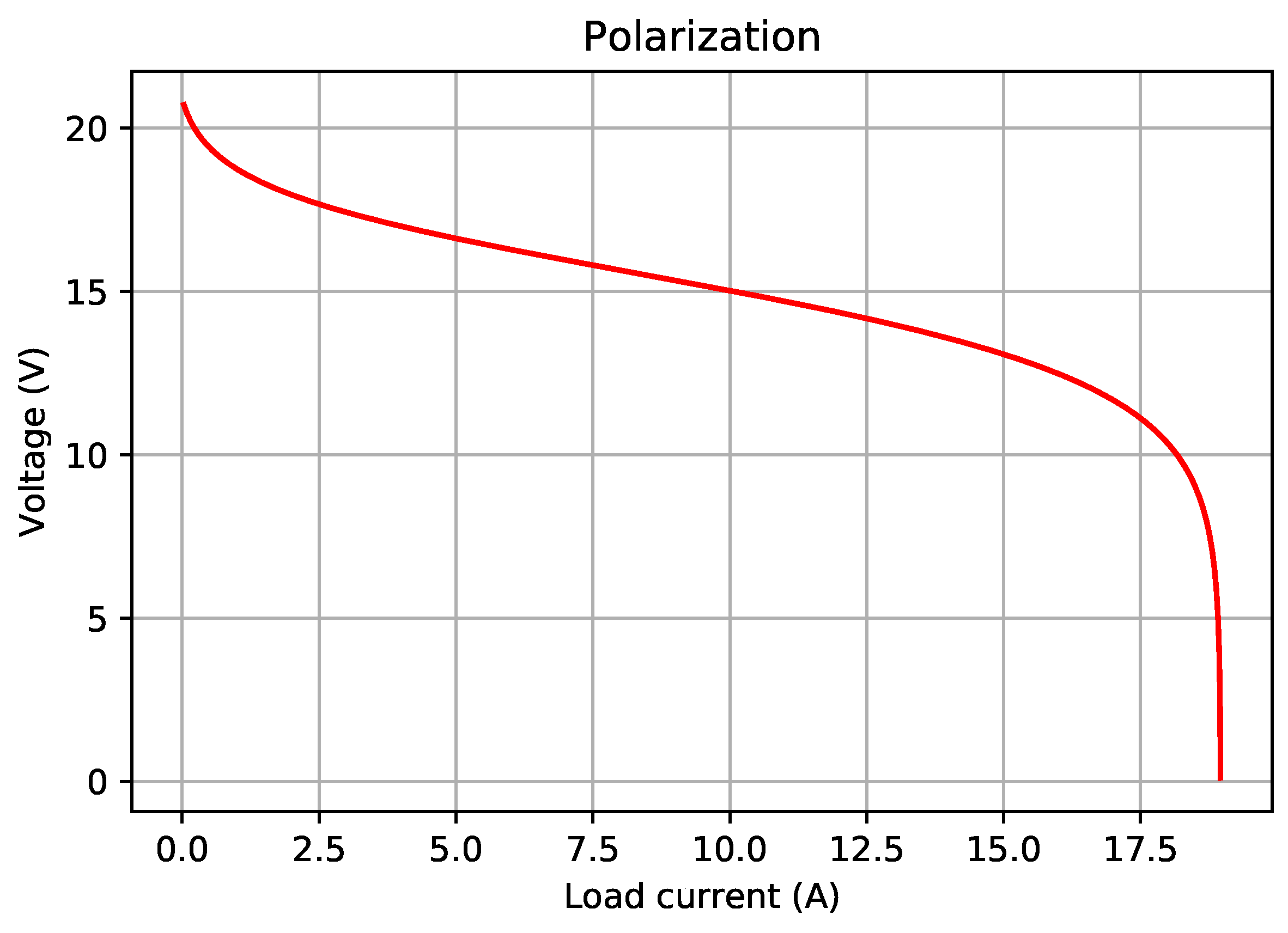
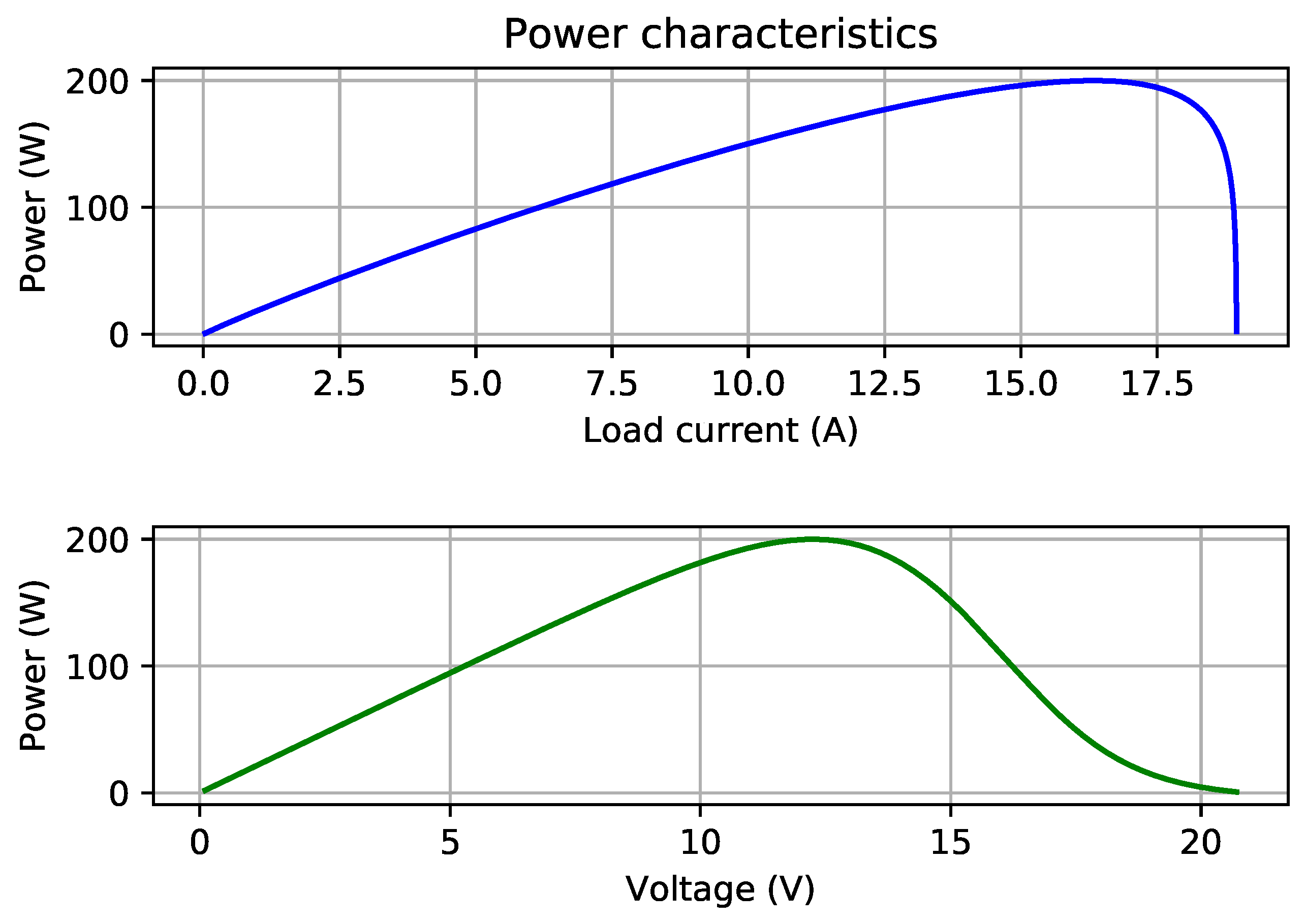
4.2. Effect of Current Step Size on Numerical Calculations of $P_{\mathrm{load},\max }$ and $V_{\mathrm{load},\mathrm{maxpp}}$

The maximum power point corresponding to a given stack configuration vector ($N_{\mathrm{s}},N_{\mathrm{p}},A_{\mathrm{cell}}$) and a given set of cell-parameter values ($i_{0,\mathrm{den}}$, etc.) cannot be obtained analytically. In other words, the problem of finding

$$\underset{i_{\mathrm{load},\mathrm{den}}}{argmax}\{V_{\mathrm{stack}}\times i_{\mathrm{load},\mathrm{den}}\},$$

with $V_{\mathrm{stack}}$ given by Equation (9), is not analytically solvable. A numerical, iterative method has been used in this paper, where a loop over current values is executed in order to numerically find an approximation to the maximum power point. Since the maximum power point needs to be determined for every single cost (objective function) evaluation, the total computation time to complete all such iterations for all runs in a test suite may not be trivial. It is, therefore, good to be able to use a relatively large step size in incrementing the current value in the loop. A large step size, however, reduces the accuracy of the computed $P_{\mathrm{load},\max }$ and $V_{\mathrm{load},\mathrm{maxpp}}$. The results presented so far in this paper used a current step of 50 mA. To study whether the step size affects the conclusions about the relative performance of the algorithms, we obtain a new set of results using a step size of 1 mA. These results, arguably more accurate than their 50 mA counterparts, are presented in Table 14, Table 15 and Table 16. A target cost of 13.62 is used in Table 15 because the previously used target of 13.5 was met by no run in the new set of results. Results of Wilcoxon signed-rank tests on the new set of data are shown in Table 17 which establishes the proposed method as significantly better than Jaya on the success rate as well as on the mean of best-of-run costs. Jaya is significantly better on the best of best-of-run costs metric, while the methods are statistically tied (the one-tail p-value is close to 0.5) on the remaining two metrics. Given the vagaries of chance, for stochastic heuristics, the average performance rather than the single best performance is generally considered to be a reliable indicator of a method’s performance. The new data, therefore, do not offer a convincing reason to argue that Jaya performs better than the proposed method. Combining the new results with the old ones for all five performance metrics, we conclude that the proposed heuristic meets or beats the Jaya algorithm.

Table 14. Comparison of the solution quality between Jaya and the proposed method. Each row corresponds to 100 independent runs. Current step size = 1 mA.

Configuration	Jaya		Proposed Algorithm
	Mean	Std Dev	Mean	Std Dev
1	14.16054	2.33381	13.95325	1.57569
2	14.78316	10.66273	15.43659	12.74582
3	13.80889	1.20404	13.63618	0.04099
4	13.79572	1.20465	13.62192	0.02035
5	13.62593	0.04068	13.61670	0.00261
6	13.62177	0.01535	13.61843	0.00338
7	13.78312	1.20555	13.61579	0.00007
8	13.62378	0.01720	13.62528	0.01814
9	13.61766	0.01845	13.61590	0.00052
10	13.61824	0.00648	13.61747	0.00191
11	13.61590	0.00056	13.61582	0.00029
12	13.61702	0.00257	13.61691	0.00180
13	13.61602	0.00112	13.61612	0.00102

Table 15. Comparison between Jaya and the proposed method on firstHitEvals and firstHitCost (each row corresponds to 100 independent runs). Current step size = 1 mA, target cost = 13.62.

Config.	Jaya					Proposed Algorithm
	#Success	firstHitEvals		firstHitCost		#Success	firstHitEvals		firstHitCost
		Mean	Std Dev	Mean	Std Dev		Mean	Std Dev	Mean	Std Dev
1	1	189.00000	-	13.61694	-	2	150.50000	47.5	13.61894	0.00076
2	44	250.11364	36.0298	13.61874	0.00093	46	242.71739	45.01288	13.61854	0.00094
3	35	327.34286	54.71795	13.61868	0.00094	48	328.79167	59.28777	13.61855	0.00092
4	69	386.49275	73.70262	13.61872	0.00093	79	373.78481	74.22778	13.61844	0.00107
5	91	539.02198	148.24289	13.61875	0.00088	95	544.06316	158.43669	13.61859	0.001
6	72	677.69444	179.15811	13.61847	0.00102	86	733.56977	168.45726	13.61869	0.001
7	97	491.21649	243.41641	13.61871	0.00095	100	424.39000	129.95975	13.61845	0.00103
8	55	1493.90909	370.95304	13.61860	0.00106	51	1469.15686	340.85891	13.61866	0.001
9	99	695.75758	351.41685	13.61851	0.00104	100	638.80000	257.61685	13.61867	0.00093
10	85	1783.22353	510.88268	13.61865	0.00101	90	1868.81111	556.65231	13.61869	0.00098
11	100	872.37000	414.07945	13.61857	0.00097	100	888.09000	548.58391	13.61867	0.00105
12	92	1904.11957	652.41631	13.61867	0.001	93	1928.41935	637.795	13.61872	0.00098
13	98	2072.31633	917.8234	13.61868	0.00099	99	2213.10101	1368.50318	13.61875	0.00098

Table 16. Best of best-of-run solutions (stack designs). Current step size = 1 mA.

Config.	Jaya						Proposed Algorithm
	Cost	${\mathit{N}}_{\mathbf{s}}$	${\mathit{N}}_{\mathbf{p}}$	${\mathit{A}}_{\mathbf{cell}}$, cm2	${\mathit{P}}_{\mathbf{load},\mathbf{max}}$, W	${\mathit{V}}_{\mathbf{load},\mathbf{maxpp}}$, V	Cost	${\mathit{N}}_{\mathbf{s}}$	${\mathit{N}}_{\mathbf{p}}$	${\mathit{A}}_{\mathbf{cell}}$, cm2	${\mathit{P}}_{\mathbf{load},\mathbf{max}}$, W	${\mathit{V}}_{\mathbf{load},\mathbf{maxpp}}$, V
1	13.61694	22	1	148.87233	200.58142	12.24681	13.61818	22	1	150.22004	202.39724	12.24680
2	13.61620	22	1	148.89873	200.61698	12.24673	13.61625	22	1	148.64410	200.27391	12.24676
3	13.61581	22	1	148.44346	200.00358	12.24674	13.61595	22	1	148.53458	200.12635	12.24674
4	13.61581	22	1	148.51622	200.10161	12.24673	13.61580	22	1	148.50711	200.08934	12.24673
5	13.61575	22	1	148.47067	200.04024	12.24673	13.61573	22	1	148.45245	200.01570	12.24673
6	13.61580	22	1	148.47983	200.05258	12.24673	13.61583	22	1	148.54354	200.13842	12.24673
7	13.61571	22	1	148.44334	200.00342	12.24673	13.61571	22	1	148.44334	200.00342	12.24673
8	13.61588	22	1	148.51630	200.10173	12.24674	13.61599	22	1	148.66197	200.29799	12.24673
9	13.61572	22	1	148.44334	200.00342	12.24673	13.61572	22	1	148.44334	200.00342	12.24673
10	13.61575	22	1	148.44338	200.00348	12.24673	13.61575	22	1	148.47067	200.04024	12.24673
11	13.61571	22	1	148.44334	200.00342	12.24673	13.61572	22	1	148.44334	200.00343	12.24673
12	13.61571	22	1	148.44334	200.00342	12.24673	13.61572	22	1	148.44334	200.00342	12.24673
13	13.61571	22	1	148.44334	200.00342	12.24673	13.61571	22	1	148.44334	200.00342	12.24673

Table 17. Wilcoxon signed rank tests on the data in Table 14, Table 15 and Table 16.

Test Description	Average of Best-of-Run Costs	No. of Successes	Mean of firstHitEvals	Mean of firstHitCost	Best of Best-of-Run Costs
Null hypothesis	Jaya-Proposed = 0	Jaya-Proposed = 0	Jaya-Proposed = 0	Jaya-Proposed = 0	Jaya-Proposed = 0
Alternative hypothesis	Jaya-Proposed > 0	Jaya-Proposed < 0	Jaya-Proposed > 0	Jaya-Proposed > 0	Jaya-Proposed > 0
No. of zero differences	0	1	0	0	4
n	13	12	13	13	9
$W+$	71	7.5	43	46	6
$W-$	20	70.5	48	45	39
W-statistic	20	7.5	43	45	6
Significance level $\alpha$	0.05	0.05	0.05	0.05	0.05
Critical W for n at $\alpha$ ≤ 0.05	21	17	21	21	8
Mean of W-statistic	45.5	39	45.5	45.5	22.5
Std. dev. of W-statistic	14.309088	12.747549	14.309088	14.309088	8.440972
z-score	−1.782084	−2.471063	−0.174714	−0.034943	−1.954751
p-value (left-tail probability)	0.037368	0.006736	0.430652	0.486063	0.025306

4.3. Proposed Algorithm vs. Point-Based Stochastic Heuristic

We now present performance comparisons of the proposed method against the heuristic of [42]. Each of the four maxEvals values reported in Table 9 of [42] corresponds to two different configurations in Table 3 of the present paper (see Table 18).

Table 18. Correspondence between [42] and the present paper on algorithm parameter settings.

maxEvals in Reference [42]	Configurations in the Present Paper
1000	5 and 6
2000	7 and 8
3000	9 and 10
4000	11 and 12

The best-cost solution vector from Table 4 on p. 536 of reference [42] is shown in Table 19 where the values of $N_{\mathrm{s}}$, $N_{\mathrm{p}}$ and $A_{\mathrm{cell}}$ are copied from [42], $P_{\mathrm{load},\max }$ and $V_{\mathrm{load},\mathrm{maxpp}}$ are computed by the iterative numerical method described in Section 4.2 (using two different values of the current step size), and the cost is computed from Equation (10).

Table 19. Best solution (stack design) of [42].

Current Step Size, mA	${\mathit{N}}_{\mathbf{s}}$	${\mathit{N}}_{\mathbf{p}}$	${\mathit{A}}_{\mathbf{cell}}$, cm2	${\mathit{P}}_{\mathbf{load},\mathbf{max}}$, W	${\mathit{V}}_{\mathbf{load},\mathbf{maxpp}}$, V	Cost
50	22	1	149.59700	201.55608	12.22855	13.43512
1	22	1	149.59700	201.55779	12.24723	13.62192

The first row of Table 19 shows that the current step of 50 mA produces a close agreement of $P_{\mathrm{load},\max }$, $V_{\mathrm{load},\mathrm{maxpp}}$ and cost values in this table with the corresponding values in Table 4 of [42]. For the rest of this subsection, therefore, results corresponding to only the 50 mA step size are used.

Table 9 of [42] and Table 4 and Table 10 of the present paper show that the proposed algorithm outperforms the algorithm of [42] in all of the following metrics: (i) best of the 100 best-of-run costs; (ii) mean of the 100 best-of-run costs; (iii) standard deviation of the 100 best-of-run costs; (iv) count (out of the one hundred) of successful runs; and (v) mean firstHitCost obtained from the successful runs (the mean firstHitCost of [42] is slightly better for one of the two cases—Configuration 11—of maxEvals = 4000).

To investigate the statistical significance, if any, of the difference between the means of the best-of-run costs of the two algorithms, we performed unpaired t-tests, the results of which are presented in Table 20. We tested the null hypothesis ${\mu }_1-{\mu }_2=0$ against the one-sided alternative ${\mu }_1-{\mu }_2>0$, where ${\mu }_1$ and ${\mu }_2$ are the (population) means of the method in [42] and the proposed method, respectively. We chose a level of significance of 0.05. Since the sample variances differ by a factor of about 10,000, the standard two-sample t-test cannot be used. We, therefore, used the Smith–Satterthwaite test [32,54] corresponding to unequal variances. The test statistic is given by

$$t-\mathrm{statistic}=\frac{{\displaystyle {\overline{x}}_1-{\overline{x}}_2-0}}{{\displaystyle \sqrt{\frac{s_1^2}{n_1}+\frac{s_2^2}{n_2}}}},$$

and its sampling distribution can be approximated by the t-distribution with

$$\frac{{\displaystyle {\left(\frac{s_1^2}{n_1}+\frac{s_2^2}{n_2}\right)}^2}}{{\displaystyle \frac{{(s_1^2/n_1)}^2}{n_1-1}+\frac{{(s_2^2/n_2)}^2}{n_2-1}}}$$

degrees of freedom (rounded down to the nearest integer), where ${\overline{x}}_1$ and ${\overline{x}}_2$ represent the two sample means, $s_1$ and $s_2$ are the two sample standard deviations, and $n_1$ and $n_2$ are the two sample sizes (100 each).

Table 20. The method in [42] versus the proposed method: results of Smith–Satterthwaite tests for comparing the means of 100 best-of-run costs for each configuration.

Configuration	Reference [42] Table 9 Row#	d.f.	t-Statistic	Critical ${\mathit{t}}_{0.05}$	95% Conf Intvl
5	1	99	3.801772	1.660	1.566897–4.987263
6	1	99	3.776139	1.660	1.544804–4.965176
7	2	99	5.193092	1.660	1.635489–3.657751
8	2	99	5.106933	1.660	1.591610–3.613910
9	3	99	4.973979	1.660	1.455472–3.387028
10	3	99	4.954752	1.660	1.446088–3.377612
11	4	99	5.112608	1.660	1.573628–3.569452
12	4	99	5.102306	1.660	1.568447–3.564273

Table 20 presents, for each configuration, the following:

• t-statistic;
• degrees of freedom (d.f.);
• the critical t value (obtained from standard tables of t-distribution) at 95% (right-tail probability of 0.05) and for the specified degrees of freedom; and
• 95% confidence interval for the difference of the two means,
  ${\overline{x}}_1-{\overline{x}}_2\pm t_{0.025}$ at the specified degrees of freedom $\times \sqrt{{\displaystyle \frac{s_1^2}{n_1}+\frac{s_2^2}{n_2}}}$.

The results show that, for each case, the t-statistic exceeds $t_{0.05}$ for the relevant degrees of freedom. Therefore, the null hypothesis is rejected in all of these cases. Furthermore, none of the confidence intervals contains zero. We thus conclude that the improvements produced by the proposed method are statistically significant.

Smith–Satterthwaite tests were also performed for comparing [42] against Jaya, and the results (see Table 21) establish Jaya as significantly better than [42].

Table 21. The method in [42] versus Jaya: results of Smith–Satterthwaite tests for comparing the means of 100 best-of-run costs for each configuration.

Configuration	Reference [42] Table 9 Row#	d.f.	t-Statistic	Critical ${\mathit{t}}_{0.05}$	95% Conf Intvl
5	1	99	3.786131	1.660	1.553444–4.973876
6	1	99	3.771733	1.660	1.541014–4.961406
7	2	110	4.729357	1.645	1.450321–3.503239
8	2	99	5.095779	1.660	1.585946–3.608274
9	3	99	4.972432	1.660	1.454715–3.386265
10	3	99	4.944366	1.660	1.441048–3.372592
11	4	99	5.111256	1.660	1.572948–3.568772
12	4	99	5.097524	1.660	1.566045–3.561875

4.4. Proposed Algorithm vs. Genetic Algorithm

The best solution produced by the genetic algorithm in [41] recommends the following stack design: $N_{\mathrm{s}}$ = 21, $N_{\mathrm{p}}$ = 1, $A_{\mathrm{cell}}$ = 156.25 cm². Plugged into Equations (9) and (10), this design yields the maximum power point value and the corresponding cost shown in Table 22 where two sets of calculations (for the two step sizes for current) were used. The proposed method’s best solutions outperform both cases in Table 22 not only on the objective function (cost) but also on the output voltage at the maximum power point: the $V_{\mathrm{load},\mathrm{maxpp}}$ values in Table 22 are less than the rated voltage of 12 V.

Table 22. Best solution (stack design) of [41].

Current Step Size, mA	${\mathit{N}}_{\mathbf{s}}$	${\mathit{N}}_{\mathbf{p}}$	${\mathit{A}}_{\mathbf{cell}}$, cm2	${\mathit{P}}_{\mathbf{load},\mathbf{max}}$, W	${\mathit{V}}_{\mathbf{load},\mathbf{maxpp}}$, V	Cost
50	21	1	156.25000	200.95239	11.69428	13.71341
1	21	1	156.25000	200.95247	11.69021	13.75418

4.5. Proposed Algorithm vs. Quasi-Analytical Approach

The best solution produced by the quasi-analytical method in [43] yields the following stack design: $N_{\mathrm{s}}$ = 22, $N_{\mathrm{p}}$ = 1, $A_{\mathrm{cell}}$ = 151.4 cm². Plugging these values into Equations (9) and (10) gives the maximum power point values and the corresponding costs in Table 23. All of the best solutions of the proposed method in Table 13 and Table 16 have a better (lower) cost than those in Table 23. The objective function minimized in [43] is the total stack area given by $N_{\mathrm{s}}{N}_{\mathrm{p}}{A}_{\mathrm{cell}}$, and yet the proposed method’s best solutions produce better (smaller) total areas, while meeting the requirements of the rated voltage and rated power.

Table 23. Best solution (stack design) of [43].

Current Step Size, mA	${\mathit{N}}_{\mathbf{s}}$	${\mathit{N}}_{\mathbf{p}}$	${\mathit{A}}_{\mathbf{cell}}$, cm2	${\mathit{P}}_{\mathbf{load},\mathbf{max}}$, W	${\mathit{V}}_{\mathbf{load},\mathbf{maxpp}}$, V	Cost
50	22	1	151.40000	203.98559	12.26406	13.79200
1	22	1	151.40000	203.98705	12.24721	13.62352

The characterization in [43] of the design vector (22, 1, 154.16) as the best design in [42] does not seem to be correct. The vector (22, 1, 154.16) is mentioned in [42] as a “typical” design, not the best or optimal design. In fact, several of the designs in Table 4 of [42] have cell areas that are smaller than 154.16 cm², with two of them even smaller than the “optimal” area of 151.4 cm² in [43]. The design (22, 1, 149.597) from Ref. [42] outperforms the “optimal” design of (22, 1, 151.4) of [43] on the cell area metric as well as on the objective (cost) function for both the step sizes (see Table 19 and Table 23).

4.6. Polarization and Power Characteristics

Figure 1 shows the polarization curve for the stack design produced by the best of best-of-run solutions of the proposed algorithm for Configuration 13 (the last row of Table 16). The corresponding power characteristics are plotted in Figure 2. The nature of these plots agrees well with that of polarization and power characteristics of typical PEM fuel cells in the literature.

Figure 1. Stack voltage vs. load current plot for the stack given by $N_{\mathrm{s}}$ = 22, $N_{\mathrm{p}}$ = 1, $A_{\mathrm{cell}}$ = 148.443337 cm², and the single-cell parameter values from Table 1.

Figure 2. Power vs. load current (top) and power vs. voltage (bottom) plots corresponding to the polarization in Figure 1. $P_{\mathrm{load},\max }$ = 200.003419 W, $V_{\mathrm{load},\mathrm{maxpp}}$ = 12.246727 V.

5. Conclusions

A PEMFC stack design problem of practical importance has been addressed in this paper. This constrained optimization problem requires finding optimal values of three parameters of the stack configuration (namely, the number of cells in series, the number of groups in parallel, and the cell area) such that the configuration delivers the rated voltage at the rated power (the load voltage at the maximum power point is to be 12 V and the maximum power is to be at least 200 W), while keeping the total cost at a minimum. A new approach has been developed, based on the Jaya algorithm and ideas from evolutionary computation, and the new approach has been empirically (that is, via numerical simulation) compared with the Jaya algorithm and with the methods in [41,42,43], using the following performance measures: (a) the best of best-of-run costs from 100 independent runs; (b) the average of the 100 best-of-run costs; (c) the standard deviation of the 100 best-of-run costs; (d) the number of cost function evaluations needed to reach a pre-determined target cost for the very first time in a run of the algorithm; and (e) the cost of the very first (earliest) solution in a run that meets (or beats) the target cost. The proposed method has been shown to outperform the three methods in [41,42,43] and is competitive with Jaya. The improvement in performance provided by the proposed algorithm has been substantiated with statistical tests of significance.

Following the authors of [41,42,43], this paper considered only a stand-alone PEM fuel cell stack. Auxiliary systems, such as heat exchangers, compressors, etc. that often significantly affect the mass, size and cost of the entire system, were not considered; the membrane type, the type of the bipolar plate material, and many operating and constructive parameters were not considered, either. Inclusion of some of these issues would be in the agenda for future research.