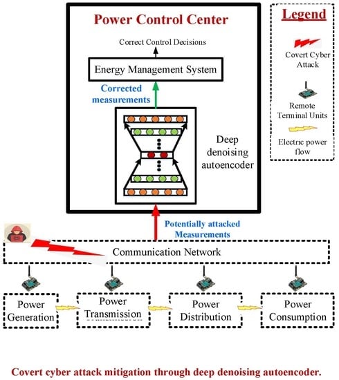
Article

Mitigating the Impacts of Covert Cyber Attacks in Smart Grids Via Reconstruction of Measurement Data Utilizing Deep Denoising Autoencoders

School of Electrical Engineering, University of Ulsan, Ulsan 44610, Korea
*
Author to whom correspondence should be addressed.
Energies 2019, 12(16), 3091; https://doi.org/10.3390/en12163091
Submission received: 5 July 2019 / Revised: 23 July 2019 / Accepted: 7 August 2019 / Published: 11 August 2019
(This article belongs to the Special Issue Cyber-Physical Systems for Smart Grids)

Abstract

:
As one of the most diversified cyber-physical systems, the smart grid has become more decumbent to cyber vulnerabilities. An intelligently crafted, covert, data-integrity assault can insert biased values into the measurements collected by a sensor network, to elude the bad data detector in the state estimator, resulting in fallacious control decisions. Thus, such an attack can compromise the secure and reliable operations of smart grids, leading to power network disruptions, economic loss, or a combination of both. To this end, in this paper, we propose a novel idea for the reconstruction of sensor-collected measurement data from power networks, by removing the impacts of the covert data-integrity attack. The proposed reconstruction scheme is based on a latterly developed, unsupervised learning algorithm called a denoising autoencoder, which learns about the robust nonlinear representations from the data to root out the bias added into the sensor measurements by a smart attacker. For a robust, multivariate reconstruction of the attacked measurements from multiple sensors, the denoising autoencoder is used. The proposed scheme was evaluated utilizing standard IEEE 14-bus, 39-bus, 57-bus, and 118-bus systems. Simulation results confirm that the proposed scheme can handle labeled and non-labeled historical measurement data and results in a reasonably good reconstruction of the measurements affected by attacks.

Graphical Abstract

1. Introduction

Integration of state-of-the-art computing and bi-directional communications technologies with the existing power infrastructure realizes the concept of the smart grid (SG) [1,2]. However, increased dependence on communications technologies is intensifying the SG’s vulnerability to cyber-attacks. Typically, a supervisory control and data acquisition (SCADA) system is employed to periodically collect data from electric power grids. The SCADA system consists of communications networks and remote terminal units (RTUs) that include sensors and actuators. At the power control center (PCC), the collected data are applied to initiate command and control decisions by the energy management system (EMS). The fitness and health of the collected data are inordinately significant when making precise and correct control decisions. Therefore, conventionally, the consistency of the sensor-collected measurement data is checked by a data detector (BDD) before being utilized in the EMS. However, a recently discovered covert cyber-deception attack (CCDA) [3] is considered competent at deceiving the conventional BDD. Smartly designing the attack vector, a malicious user can compromise the integrity of the SG by injecting biased values into the sensor measurement data to dodge the BDD with a false, yet feasible system state [3]. Thus, initiating the CCDA through biased data may end in financial loss, partial disruption in power system operations, or a compound of economic loss and disruptions [4,5]. Owing to the harmful impacts of such attacks on the reliable and secure operations of SGs, there is a need to investigate counter attack measures.
Generally, the defense measures reported in the literature can be organized into three layers: protection, detection, and mitigation [6].
Extensive investigations have been reported in the literature on the detection layer of the defense mechanism. Table 1 shows a summary of the research works carried out on the detection and mitigation tiers. In Table 1, it can be seen that less attention has been paid by researchers to the mitigation tier. Particularly, in the context of CCDA attack mitigation through the reconstruction of sensor collected measurement data, there is no existing work to the best of our knowledge. In the context of self-healing [7], which is a significant characteristic of an SG, there is a need to focus on mitigation layer and neutralize or minimize the impacts of a CCDA.
Figure 1 explains the prevailing circumstances and conceivable mitigations for CCDAs. We can see in Figure 1 that the sensor-collected data samples are scrutinized by the intrusion detection system (IDS). The data identified as normal by the IDS are considered reliable enough to employ in the EMS to make control decisions. On the other hand, the data sample detected by IDS as attacked cannot be applied to the decision process. Due to the lack of any convincing solution, the attacked data sample is currently dropped, and the next sample is awaited, as depicted by Scheme-I in Figure 1. The same procedure is repeated, delaying control decisions until attack-free samples are received. However, due to the introduction of distributed generation and dynamically varying load conditions, taking immediate control decisions is desired for reliable and economic operations of power grids. Therefore, removing the impacts of a CCDA from corrupted measurement data is a more valuable solution than discarding samples. In this context, there is a need to establish a mechanism to induce a self-healing capability [7,32,33] in the PCC, which removes bias added by an intruder. As shown by Scheme-II in Figure 1, one possible option is to reconstruct the corrupted sample after its detection, which involves both detection and reconstruction time. An alternative is to reconstruct the data sample directly, omitting the detection stage, as shown by Scheme-III in Figure 1. Thus, the time consumed in detection can be saved; however, all measurement samples are reconstructed in this scheme, whether they were attacked or not. Table 2 shows a comparison of the above-mentioned mitigation schemes.
To extend our previous work from detection [6,25,26] to mitigation, in this paper, we propose a deep neural network (DNN)-based data reconstruction scheme (Scheme-III) to mitigate the impacts of a CCDA on the SG’s measurement dataset.

1.1. Motivation

Due to the vast geographical spans of power transmission networks, many sensors are deployed to collect the state data. Machine learning (ML)-based approaches may directly utilize the sensor measurements to mitigate the effects of CCDAs without requiring precise mathematical modeling. Additionally, ML-based mitigation through the reconstruction of the data does not need antecedent information of the power network. Furthermore, the state estimation (SE) measurement features (MF) data from power transmission networks via multiple sensors are multivariate and extremely correlated due to synergy and interaction between interconnected buses. Legacy multivariate-procedure monitoring techniques, such as principal component analysis (PCA) and an autoencoder (AE) with linear activation, assume linear process behavior that may not be suitable for SE-MF data. Moreover, PCA and AE are more sensitive to corruption in the data, and they have not adapted to learning robust representation from data corrupted due to attacks. In this paper, we present an SE-MF data reconstruction scheme based on a recently developed denoising autoencoder (DAE) to address the aforesaid challenges. Recent studies [34,35,36] have shown that a DAE can reconstruct the original signal by learning more robust representations from the attacked data. A comparison between the DAE and PCA is presented in Table 3. Inspired by its efficient application and magnificent characteristics for dealing with corrupted multivariate SE-MF data, we utilize the DAE for the robust reconstruction of attacked measurement samples while learning the nonlinear correlations embedded in an SE-MF dataset.

1.2. Contributions

In this paper, we consider multivariate SE-MF data affected by a CCDA. To reconstruct data by removing bias added by an attacker, we employ a state-of-the-art anomaly reconstruction method: the denoising autoencoder. The major technical contributions of this paper are summarized as follows.
  • We investigate the impacts of smartly crafted CCDA on SG measurements, and study how such an attack can sidestep a BDD in typical power systems.
  • We introduce the DAE algorithm to capture in a more robust way nonlinear correlations in multivariate SE-MF data corrupted by CCDA attacks while setting out robust signal reconstruction. To the best of our knowledge, this is the first paper to employ a DAE for reconstruction of corrupted sensor measurements in SE-MF data from SGs.
  • To train the DAE model, commonly used choices for the addition of corruption are the zero-masking DAE (ZDAE) and the additive Gaussian DAE (GDAE) [27]. In addition to these schemes, we have introduced another corruption-addition scheme termed estimated DAE (EDAE). A comparison of these schemes shows that the newly introduced EDAE trains the denoising autoencoder model to obtain robust and powerful representations from the raw attacked data and results in a low reconstruction error.
  • We employ IEEE standard 14-bus, 39-bus, 57-bus, and 118-bus test systems to gauge the performance of the proposed approach. Performance evaluations show that the proposed EDAE scheme results in reasonably good reconstruction with little loss of accuracy.

1.3. Paper Organization

The rest of this paper is organized as follows. In Section 2, state estimation, conventional bad data detection, and the nature of a CCD attack on an SG network are presented. In Section 3, we explain the fundamentals of the DAE, followed in Section 4 by an explanation of the proposed scheme to reconstruct the sensor measurements corrupted by a CCDA. Simulation results are presented in Section 5. We conclude the paper in Section 6.

2. System Model

2.1. Electric Power Network

The power transmission system connects various electrical generators across a vast geographic region with a host of customers. Multiple routes and lines contribute to securing the routing of the power from any generating source to any consumer, considering the economy of the transmission route. For effective monitoring and control of the power infrastructure, a communications network linking the power system components to the PCC is employed.

2.2. State Estimation

For the purpose of efficient monitoring, bi-directional RTUs, consisting of sensors and actuators, are employed in the power network. The readings of the sensors are collected at the PCC, which estimates the states (bus voltage angles and magnitudes) of the power system variables by utilizing the sensor measurements. The problem is to estimate the state variables, θ = x 1 , x 2 , , x n T , considering the sensor-collected measurements, Z = m 1 , m 2 , , m m T , of the power system, where n and m are positive integers, and x i , m j I R for i = 1 , 2 , , n and j = 1 , 2 , , m . More specifically, the state variables are connected with the measurements in a nonlinear or alternating current (AC) model as follows:
Z = h ( θ ) + e
where h is a nonlinear relationship between measurement vector Z and state vector, and e = [ e 1 , e 2 , , e m ] T is a Gaussian measurement noise vector with standard deviation σ . On the assumption that the voltage magnitude at each bus remains close to its rated value, the model in Equation (1) can be described utilizing direct current (DC) model as follows:
Z = H θ + e
where H is the Jacobian matrix in DC power flow problems and is approximated as follows [40,41]:
H = h ( θ ) θ θ = 0 .
H is composed of topology and impedance data only. To find the estimate, θ ^ , of the θ that is the best fit of the measurements, three statistical criteria are utilized in state estimation: maximum likelihood, minimum variance and weighted least squares (WLS) [42]. On the assumption that sensor error is normally distributed with a zero mean, the above-mentioned criteria result in an identical voltage phase estimation, as follows:
x ^ = ( H T Ω H ) 1 H T Ω Z = G Z ,
where G = ( H T Ω H ) 1 H T Ω , and Ω is a diagonal matrix where the elements are reciprocals of the variances in meter errors.
Ω = σ 1 2 . . . σ m 2 ,

2.3. Conventional Bad Data Detection

The sensor-collected measurement data may become corrupted for many reasons, such as sensor faults, communication medium noise, and cyber attacks. Sensor-collected measurements result in an estimate of the state variables that is close to their true values under normal conditions, whereas a CCDA attack may result in shifted state variables, introducing a contrariety between the normal and attacked measurements. Typical power systems employ a residual-based detector to identify corruptions in the sensor measurements [3]. The residual, R, is the difference between sensor collected measurements, Z , and the estimated measurements, Z ^ , at the PCC, and is described as follows:
R = Z Z ^ = Z H θ ^ .
Then, L 2 n o r m   Z H θ ^ is compared with a deliberately selected threshold, τ [11], to detect the presence of bad measurements. Therefore, the hypothesis of not being attacked is accepted if we have
max i R i < τ ,
where R i is the element of residual vector R. Otherwise, an alarm indicating existence of bad measurements is raised.

2.4. Covert Cyber Deception Attack: Basic Principle

From a complete (or even partial) familiarity with the power network topology, a smart attacker can add biased data to meter or sensor-collected measurements Z by forming an attack vector, a = [ a 1 , a 2 , , a m ] T , to deceive the bad data detector [27]. Let Z a = Z + a be the measurements containing the attacked data. In attack vector a, the attacker enjoys the liberty of selecting any non-zero arbitrary element. Thus, the i th non-zero element, a i , of attack vector a, allows that the attacker to alter the i th sensor measurement, Z i , with a forged measurement: Z i + a i .
As discussed above, the conventional bad data detector computes the L 2 norm of measurement residual R, to determine the presence of attacked or bad measurements. However, if the attacker designs attack vector a, such that a = H c , where c is a non-zero vector of length n, the measurement vector containing the attacks Z a can circumvent the traditional detection as long as the measurement vector containing the normal measurements can pass.
Let θ ^ a denote an estimate of state variables using attacked sensor measurements Z a such that we have
θ ^ a = G Z + G a = θ ^ + G H c = θ ^ + c .
Now, the L 2 norm of attacked measurements residual R a is
R a 2 = Z a H θ ^ a 2 = ( Z + a ) H ( θ ^ a + c ) = Z H θ ^ + a H c 2 = Z H θ ^ 2 = R 2 < τ .

2.5. Covert Cyber Deception Attack Model

Broadly speaking, there are two kinds of CCD attack: (1) the load redistribution attack; and (2) the load change attack [43,44,45]. With the ultimate objective being to dodge the conventional BDD and pass the operator at the PCC, the attacker may craft the attack aiming at altering one or more measurements. In this paper, our main objective is real-time reconstruction of corrupted sensor measurements. Therefore, our approach is to formulate the most generalized attack, and thereby to come up with robust reconstruction of the attacked measurements. For the construction of the attack, we assumed that the assailant has enough knowledge about the power network topology.
During the CCD attack, the malicious user embeds a forged value in the sensor measurements, altering the real power injection and real power flows to project the desired changed state variables for the system operator. For instance, to change state variable x 2 by adding a corruption of −12%, a ( 1 × ( n 1 ) ) attack vector c can be formulated by considering the following equation:
c = [ 0.12 x 2 , 0 , , 0 ] .
Utilizing the power flow equations and state vector x a = x ^ + c , the corrupted measurements are calculated as follows:
Z a = H θ a + e .

3. Reference Model Learning

In this section, we first briefly describe the AE and denoising autoencoder (DAE) algorithm, and then, we explain the proposed data reconstruction scheme.

3.1. Autoencoder: Basic Principle

Autoencoders (AEs) are a specific type of fully connected feed-forward neural networks where the inputs are equal to the output, and therefore, the AE is trained in an unsupervised way without any label information. Fundamentally, an AE consists of three elements: an encoder, the code, and a decoder. The encoder compresses the input into a lower-dimensional code or latent-space representation, and then, the decoder reconstructs the output from this representation. Analogous to PCA, the AE aims to encode the input data into an intermediate representation that preserves most of the information in the input data to allow reconstructing it. In this paper, to capture the hidden nonlinear correlations more robustly, and to tackle a CCDA in complex multivariate data, we employ a recently developed algorithm in the field of deep learning, the DAE [39]. The DAE is an expansion of the AE and has multiple advantages over the conventional PCA-based dimension-reduction method, as explained in Table 2.

3.2. Denoising Autoencoder: Basic Principle

The fundamental concept of the DAE is to reconstruct the primary input from corrupted or attacked input [39]. Thus, it can stop an AE from just learning identity mapping between the input and the reconstructed output, can apprehend more informational latent-space patterns, and can gather a strong and robust representation from raw, attacked data. Two primary choices for addition of corruption are additive Gaussian noise (the GDAE) and zero-masking noise (the ZDAE) [34].
Similar to AE, a DAE is composed of three parts: the encoder, code or latent space, and the decoder. Given an input, x, the encoder typically transforms its corrupted or attacked input data, x ˜ , instead of original input data x, into a hidden or latent-space representation, h, employing nonlinear mapping as follows:
h = f W 1 x + b ,
where f ( . ) is a nonlinear activation function, such as the sigmoid function. W 1 I R m × n is the weight matrix, and b I R m is optimized in the encoding with m nodes in latent space. Then, the decoder unfolds the latent space into a reconstructed vector, x ^ , at the output layer, utilizing nonlinear transformation as follows:
x ^ = g W 1 x + c ,
where g ( . ) is a nonlinear activation function, such as the sigmoid function. For better learning efficiency, we employed the tied weights as W 1 = W 2 T [39]. The reconstruction error can be computed for a given input training set, x i i = 1 m , as follows: i = 1 m x i x ^ i 2 . The objective training of the DAE is to find optimal parameters, ψ = W 1 , b , c that minimize the reconstruction error, as given below:
min ψ i = 1 m x i x ^ i 2 .
It is obvious from Equation (13) that the reconstruction error is the difference between the reconstructed output and the actual meter measurements instead of the attacked measurements. In other words, the DAE is trained to produce output closer to the original input x, even when employing the attacked input, x ˜ .

4. Proposed CCDA Mitigation–Data Reconstruction Scheme

Recovering the original sensor measurements from the attacked signals is required for a self-healing SG. In this section, we propose a scheme utilizing a DAE for the reconstruction of measurements corrupted due to a CCDA in an SG communications network. Figure 2 illustrates the reference model’s learning process. The bulk power-generated at the power producing plants is transported to consumers via the power transmission and distribution networks. The RTUs collect measurement data X 0 from the power network and transmit the collected data over wireless media. A smart attacker can compromise the integrity of the data by adding biased values to the collected data. At the power control center, the proposed DAE-based reconstruction scheme attempts to reconstruct the attacked data, X ˜ 0 , by removing any bias added by the attacker. A healthy DAE model reconstructs the data well enough to be employed in the EMS for initiating command and control decisions. The proposed reconstruction scheme is explained in the following subsection. Figure 3 shows the flowchart of the proposed scheme.

4.1. Proposed Corruption Addition Scheme: EDAE

As mentioned above, there are two common choices of adding corruption to the DAE model for training: the ZDAE and GDAE [34]. In the ZDAE scheme, some features of each sample are set to zero randomly with probability v. Practically speaking, zero-masking can be viewed as the nonexistence of sensor measurements (due to attack or noise). In addition to the above-mentioned choices, in this paper, we introduce another corruption addition scheme EDAE, in which the noise is generated based on Gaussian distribution with mean and variance obtained from analysis of the SE-MF data. The corruption addition procedure following the EDAE is explained as follows.
To train the DAE model, we insert noise or corruption to the SE-MF training data X = x 1 , x 2 , , x m , where m is the number of measurement samples, and x i X , where i 1 , 2 , , m . The x i is a sample consisting of n features, x i = f i 1 , f i 2 , , f i n . The corruption or noise data δ follows a normal distribution N μ , ν , where μ is a vector of mean values μ = μ 1 , μ 2 , , μ n , which is calculated as μ j = 1 m i = 1 m f i j . The ν is a variance vector ν = ν 1 , ν 2 , , ν n where ν j = 1 m i = 1 m μ j f i j 2 . Finally, the training data are obtained as X 0 = X + δ , and used for training the DAE model.

4.2. DAE Model Training

Let x 0 X 0 be the historical SE-MF input data, where X 0 I R m × n . To train the DAE model to minimize any loss in the reconstruction process, we insert normal (attack-free) data, y 0 Y 0 , as labels, where Y 0 I R m × n , in which m is the number of measurement samples, and n is the number of measurement features in a sample.
Before employing the input data to train the learning model (i.e., the DAE), data normalization is required as a pre-processing step; otherwise, the data are not reconstructed well enough. Data normalization means converting all variables in the data within a particular range. Normalization is essential for steady convergence of weights and biases. There are several types of normalization, such as min-max normalization, decimal scaling, and the standard deviation method [46,47]. Choosing a suitable normalization method depends on the application and the algorithm in which the normalized data will be used. The min-max normalization approach is a simple normalization technique and is usually more efficient. To linearly scale each feature to the range 0 1 , in this paper, we employ a min-max normalization function as follows [46]:
f ˜ i = f i f min f max f min ,
where f ˜ i is the normalized, or scaled, value of feature i, and f min and f max are the minimum and maximum values, respectively, of feature i in the dataset. Normalization of training and testing data according to the same scale helps in a good reconstruction. After normalization, the data are inserted to train the DAE model. Equations (1)–(3) are applied to the input data to find the optimal parameters defined by ψ , and to acquire the hidden representation h and the rebuilt output by minimizing the reconstruction error as follows: min x ^ 0 y 0 f o r X 0 , Y 0 .

4.3. DAE Model Testing

During the testing phase, online data are inserted to the trained DAE model. The test samples are also rescaled according to the minimum and maximum values of the training data, ensuring both datasets are in a similar range. A trained DAE model attempts to reconstruct the test data identical to the normal data. Each feature in the reconstructed data is denormalized using the inverse transformation, as follows:
f i = f ˜ i f max f min + f min .
A well-trained, healthy DAE will generate the reconstructed data as close to the original input as possible and the reconstructed data can be employed in the EMS with high enough level of confidence to initiate control decisions.

5. Experimental Results

In this section, we gauge the performance of the proposed reconstruction scheme for CCDA-corrupted data.

5.1. Power System Data and Attack Data Generation

We utilized various power system test cases, from standard IEEE 14-, 39-, 57-, and 118-bus systems, to endorse the performance of the proposed mitigation scheme. To set up the configuration of these standard IEEE test systems, and explicitly the Jacobian matrix, we applied the Matpower 6.0 toolbox [48]. To generate the measurements, Z, operating points of the test systems provided in Matpower case files were employed. We used the DC power flow analysis to approximate the state vectors employed in the AC power flow model. The state variable vector θ , for a B-bus system, consists of ( B 1 ) bus voltage phase angles, and measurement vector Z comprises of active power flows in the lines and active power injections into the buses. To carry out a fair comparison with a real-world power system, we adopted stochastic loads with uniform load distributions identical to those in [24], i.e., ranging from 0.9 × Q 0 to 1.1 × Q 0 , where Q 0 is the base load. The features employed in these simulations were the active power flows in the branches and active power injections into the buses.
As mentioned above, the CCDA can be modeled to deceive the BDD with the ultimate objective being to falsify single or multiple system states. We assumed that the attacker has complete knowledge of the topology of the power network, and the attack is initiated following the model described in [6]. The attack formulation is explained in Section 2. In the simulations, we considered various attack scenarios, described as follows.
Scenario 1: The attacker is stationary and has access to specific RTUs or meters only. Thus, the attacker can initiate a fixed attack, i.e., fixed or the same features in the measurement samples are corrupted with the attack.
Scenario 2: The attacker is moving and can randomly access different RTUs or meters. Initiating such an attack, the attacker randomly adds biased values into the features or meter measurements. This sort of attack is stronger than a fixed attack, and arduous for the recovery of the original data through reconstruction. For the above-mentioned fixed- and random-attack scenarios, the measurement data attacks were on 40% of the features and 20% of the features.

5.2. Parameter Tuning for the DAE Structure

We employed multiple power system test cases to validate the performance of the proposed SG data-reconstruction scheme. Power variable states and measurement features for standard IEEE systems increase as the size of the power system increases. Therefore, for each power system test case, the DAE structure has a different number of input nodes. The DAE reconstructs the output so it is identical to original input; therefore, the number of input and output nodes in a DAE structure is the same. We used 50% of the historical SE-MF data for training the DAE model and 50% for testing it. For each standard IEEE test bus system employed in this work, tuning parameters were chosen based on optimal reconstructed data. The simulation parameters for the DAE structure in various test bus cases are shown in Table 5. If familiar with the topology of the power system network, an attacker can adopt various strategies to dilute SG measurements. Keeping in mind an expanded attack choice for of the attacker, we employed different corruption addition schemes: the GDAE, ZDAE, and EDAE. In the following subsection, we present the simulation results for various standard IEEE test bus systems.

5.3. Simulation Results

The accuracy of the reconstructed measurements is significantly important for making correct decisions at the PCC. Therefore, the reconstruction error and error average sum (EAS) were considered performance measuring metrics for the proposed data reconstruction schemes. We simulated the system for standard IEEE 14-, 39-, 57-, and 118-bus systems, as mentioned above. However, we present simulation results only from the standard IEEE 14- and 39-bus systems due to space limitations.

5.3.1. Reconstruction Errors for Fixed- and Random-Attack Dataset

As mentioned in Table 4 and Table 5, the IEEE 14-bus system has 53 measurement features, and it is challenging to present reconstruction of all the features in the dataset due to space limitations. Therefore, to show the performance of the proposed cyber-attack-mitigation scheme, the seven best and the seven worst reconstructed features are presented for the proposed EDAE and the existing ZDAE and GDAE schemes. The fixed and random attacks targeted either 20% or 40% features in the dataset. Furthermore, fixed- and random-attack scenarios were also considered in the simulations. The seven best-reconstructed features for the measurement data, in which a fixed attack was initiated on 20% of the features, are shown in Table 6 for the EDAE model. Actual values of the features and the reconstructed values (along with the reconstruction error) are shown. The error ratio is also presented in the table. A reduced error ratio is essential for attack mitigation in the SG measurement data. We see that features have been reconstructed well, because the reconstruction error and the error ratio are very small. The seven worst-reconstructed features are depicted in Table 7 for the EDAE scheme when 20% of the features were targeted in a fixed attack. We see that the reconstruction error and the error ratio are low for the reconstructed features, except for features with values closer to zero. Table 8 and Table 9, respectively, show the seven best- and worst-reconstructed features with the EDAE scheme for the data in which 40% of the features were subjected to a fixed attack. Similarly, Table 10, Table 11, Table 12 and Table 13 show the reconstruction of the data affected from a fixed attack on 20% of the features and 40% of the features, for the ZDAE schemes. In addition, Table 14, Table 15, Table 16 and Table 17 show GDAE scheme’s reconstructed data that were subjected to fixed attack. Similarly, from random attacks, the seven best-, and worst-reconstructed features are shown in Table 18, Table 19, Table 20, Table 21, Table 22, Table 23, Table 24, Table 25, Table 26, Table 27, Table 28 and Table 29 for the earlier-mentioned DAE schemes. We see that features have been reconstructed well, because the reconstruction error and the error ratio are small for the EDAE scheme, compared to the other schemes.
Discussion: In Table 6, Table 7, Table 8, Table 9, Table 10, Table 11, Table 12, Table 13, Table 14, Table 15, Table 16, Table 17, Table 18, Table 19, Table 20, Table 21, Table 22, Table 23, Table 24, Table 25, Table 26, Table 27, Table 28 and Table 29, it is observed that all features have been reconstructed well with the EDAE scheme, compared to other schemes. However, the error ratio is high for the features with values closer to zero. These results were obtained by using the mean squared error (MSE) objective function. It would be interesting future work to reduce the error ratio by investigating more objective functions.

5.3.2. Error Average Sum (EAS)

Next, to show the reconstruction performance in the overall dataset, we present average error sum (EAS) as another performance gauge. The average error sum is given as follows: 1 m i = 1 m e i , where m is the number of features and e i is the reconstruction error for the ith feature. The EAS is measured in megawatts (MW). Figure 4, Figure 5, Figure 6, Figure 7, Figure 8, Figure 9, Figure 10 and Figure 11 show the EAS for the various DAE schemes for the 20% and 40% fixed-attacked features from the standard IEEE 14-, and 39-bus systems.
Discussion: It is observed that the proposed EDAE scheme has the lowest reconstruction error, compared to the other schemes. The ZDAE outperforms the GDAE, which has the highest reconstruction error.

5.3.3. Training and Validation Costs

Figure 12, Figure 13, Figure 14, Figure 15, Figure 16, Figure 17, Figure 18 and Figure 19 show the reconstruction error on the training data as a function of the number of epochs for 20% and 40% fixed- and random-attack datasets. These results are shown for standard IEEE 14- and 39-bus systems. The training and validation cost is measured in megawatts (MW).
Discussion: The results of the training and validation cost show that the proposed EDAE scheme results in much less reconstruction error, compared to the ZDAE and GDAE schemes for all test bus cases. It is also observed in the figures that the reconstruction performance of ZDAE is better as compared to the one achieved by the GDAE scheme.
From the overall results, we also observe that, during the reconstruction process, the EDAE scheme performs better than other schemes. The reconstruction error, EAS, and training and validation costs are the lowest in the case of the proposed EDAE-based reconstruction scheme.

6. Conclusions

In this paper, we propose a DAE-based scheme to reconstruct the measurements affected by a covert cyber-deception attack while removing the added biased values. We considered different corruption-addition schemes, such as zero-masking (the ZDAE), additive Gaussian noise (the GDAE), and an estimated corruption-addition (termed the EDEA), under diverse attack scenarios. The performance of the proposed scheme was evaluated by employing standard IEEE 14-bus, 39-bus, 57-bus, and 118-bus systems. Active power injections into the buses and active power flow measurements in the branches are the main features of the dataset. The test results show that the proposed EDAE-based reconstruction scheme results in a reasonably low reconstruction error from CCDAs on SG measurement features. Furthermore, the proposed EDAE-based reconstruction scheme results in a low error ratio, compared to the other schemes. However, the features with values closer to zero are reconstructed with a high error ratio. The results were obtained using an MSE objective function. In the future, to further reduce the error ratio for features with small values, we intend to investigate more objective functions in order to increase the reconstruction accuracy.

Author Contributions

All authors conceived and proposed the research idea. S.A. and Y.L. designed the experiments; S.A. performed the experiments; S.-H.H. and I.K. analyzed experimental results; and S.A. wrote the paper in the supervision of S.-H.H. and I.K.

Funding

This research was funded by Basic Science Research Program through the National Research Foundation of Korea (NRF) funded by the Ministry of Education (2016R1A6A3A11932461).

Conflicts of Interest

The authors declare no conflict of interest.

References

  1. Ahmed, S.; Lee, Y.D.; Hyun, S.H.; Koo, I. A Cognitive Radio-Based Energy-Efficient System for Power Transmission Line Monitoring in Smart Grids. J. Sens. 2017, 2017, 3862375. [Google Scholar] [CrossRef]
  2. Ahmed, S.; Usman, M.; Koo, I. Sensor node selection-based lifetime maximization in sensor network assisted cognitive radio networks. Adv. Sci. Lett. 2016, 22, 2432–2437. [Google Scholar] [CrossRef]
  3. Liu, Y.; Ning, P.; Reiter, M.K. False data injection attacks against state estimation in electric power grids. ACM Trans. Inf. Syst. Secur. (TISSEC) 2011, 14, 13. [Google Scholar] [CrossRef]
  4. Khanna, K.; Panigrahi, B.K.; Joshi, A. Data integrity attack in smart grid: Optimised attack to gain momentary economic profit. IET Gener. Transm. Distrib. 2016, 10, 4032–4039. [Google Scholar] [CrossRef]
  5. Liu, X.; Li, Z. Local load redistribution attacks in power systems with incomplete network information. IEEE Trans. Smart Grid 2014, 5, 1665–1676. [Google Scholar] [CrossRef]
  6. Ahmed, S.; Lee, Y.; Seung-Ho, H.; Koo, I. Unsupervised Machine Learning—Based Detection of Covert Data Integrity Assault in Smart Grid Networks Utilizing Isolation Forest. IEEE Trans. Inf. Forensics Secur. 2019, 14, 2765–2777. [Google Scholar] [CrossRef]
  7. Cinar, M.; Kaygusuz, A. Self-Healing in Smart Grid: A Review. Bitlis Eren Üniversitesi Fen Bilimleri Dergisi 2018, 7, 492–503. [Google Scholar] [CrossRef]
  8. Mo, Y.; Chabukswar, R.; Sinopoli, B. Detecting integrity attacks on SCADA systems. IEEE Trans. Control Syst. Technol. 2014, 22, 1396–1407. [Google Scholar]
  9. Vamvoudakis, K.G.; Hespanha, J.P.; Sinopoli, B.; Mo, Y. Detection in adversarial environments. IEEE Trans. Autom. Control 2014, 59, 3209–3223. [Google Scholar] [CrossRef]
  10. Mo, Y.; Weerakkody, S.; Sinopoli, B. Physical authentication of control systems: Designing watermarked control inputs to detect counterfeit sensor outputs. IEEE Control Syst. 2015, 35, 93–109. [Google Scholar]
  11. Lin, H.; Slagell, A.; Kalbarczyk, Z.; Sauer, P.; Iyer, R. Runtime semantic security analysis to detect and mitigate control-related attacks in power grids. IEEE Trans. Smart Grid 2016, 9, 163–178. [Google Scholar] [CrossRef]
  12. Sridhar, S.; Govindarasu, M. Model-based attack detection and mitigation for automatic generation control. IEEE Trans. Smart Grid 2014, 5, 580–591. [Google Scholar] [CrossRef]
  13. Hong, J.; Liu, C.C.; Govindarasu, M. Integrated anomaly detection for cyber security of the substations. IEEE Trans. Smart Grid 2014, 5, 1643–1653. [Google Scholar] [CrossRef]
  14. Yang, Y.; McLaughlin, K.; Sezer, S.; Littler, T.; Pranggono, B.; Brogan, P.; Wang, H. Intrusion detection system for network security in synchrophasor systems. In Proceedings of the IET International Conference on Information and Communications Technologies (IETICT 2013), Beijing, China, 27–29 April 2013. [Google Scholar]
  15. Fan, Y.; Zhang, Z.; Trinkle, M.; Dimitrovski, A.D.; Song, J.B.; Li, H. A cross-layer defense mechanism against GPS spoofing attacks on PMUs in smart grids. IEEE Trans. Smart Grid 2015, 6, 2659–2668. [Google Scholar] [CrossRef]
  16. Mitchell, R.; Chen, R. Behavior-rule based intrusion detection systems for safety critical smart grid applications. IEEE Trans. Smart Grid 2013, 4, 1254–1263. [Google Scholar] [CrossRef]
  17. Zhang, Y.; Wang, L.; Sun, W.; Green, R.C., II; Alam, M. Distributed intrusion detection system in a multi-layer network architecture of smart grids. IEEE Trans. Smart Grid 2011, 2, 796–808. [Google Scholar] [CrossRef]
  18. Fadlullah, Z.M.; Fouda, M.M.; Kato, N.; Shen, X.; Nozaki, Y. An early warning system against malicious activities for smart grid communications. IEEE Netw. 2011, 25, 50–55. [Google Scholar] [CrossRef] [Green Version]
  19. Huang, Y.; Tang, J.; Cheng, Y.; Li, H.; Campbell, K.A.; Han, Z. Real-time detection of false data injection in smart grid networks: An adaptive CUSUM method and analysis. IEEE Syst. J. 2014, 10, 532–543. [Google Scholar] [CrossRef]
  20. Sial, A.; Singh, A.; Mahanti, A.; Gong, M. Heuristics-Based Detection of Abnormal Energy Consumption. In Proceedings of the International Conference on Smart Grid Inspired Future Technologies, Auckland, New Zealand, 23–24 April 2018; pp. 21–31. [Google Scholar]
  21. Sial, A.; Singh, A.; Mahanti, A. Detecting anomalous energy consumption using contextual analysis of smart meter data. Wirel. Netw. 2019. [Google Scholar] [CrossRef]
  22. Saini, S.; Arjunan, P.; Singh, A.; Nambiar, U. E-adivino: A novel framework for electricity consumption prediction based on historical trends. In Proceedings of the 2015 ACM Sixth International Conference on Future Energy Systems, Bangalore, India, 14–17 July 2015; pp. 213–214. [Google Scholar]
  23. Ozay, M.; Esnaola, I.; Vural, F.T.Y.; Kulkarni, S.R.; Poor, H.V. Machine learning methods for attack detection in the smart grid. IEEE Trans. Neural Netw. Learn. Syst. 2016, 27, 1773–1786. [Google Scholar] [CrossRef]
  24. Esmalifalak, M.; Liu, L.; Nguyen, N.; Zheng, R.; Han, Z. Detecting stealthy false data injection using machine learning in smart grid. IEEE Syst. J. 2014, 11, 1644–1652. [Google Scholar] [CrossRef]
  25. Ahmed, S.; Lee, Y.; Hyun, S.H.; Koo, I. Covert Cyber Assault Detection in Smart Grid Networks Utilizing Feature Selection and Euclidean Distance-Based Machine Learning. Appl. Sci. 2018, 8, 772. [Google Scholar] [CrossRef]
  26. Ahmed, S.; Lee, Y.; Hyun, S.H.; Koo, I. Feature Selection—Based Detection of Covert Cyber Deception Assaults in Smart Grid Communications Networks using Machine Learning. IEEE Access 2018, 6, 27518–27529. [Google Scholar] [CrossRef]
  27. Singh, S.K.; Khanna, K.; Bose, R.; Panigrahi, B.K.; Joshi, A. Joint-Transformation-Based Detection of False Data Injection Attacks in Smart Grid. IEEE Trans. Ind. Inform. 2018, 14, 89–97. [Google Scholar] [CrossRef]
  28. He, Y.; Mendis, G.J.; Wei, J. Real-time detection of false data injection attacks in smart grid: A deep learning-based intelligent mechanism. IEEE Trans. Smart Grid 2017, 8, 2505–2516. [Google Scholar] [CrossRef]
  29. Chen, G.; Dong, Z.Y.; Hill, D.J.; Xue, Y.S. Exploring reliable strategies for defending power systems against targeted attacks. IEEE Trans. Power Syst. 2010, 26, 1000–1009. [Google Scholar] [CrossRef]
  30. Chen, P.Y.; Cheng, S.M.; Chen, K.C. Smart attacks in smart grid communication networks. IEEE Commun. Mag. 2012, 50, 24–29. [Google Scholar] [CrossRef]
  31. Ma, C.Y.; Yau, D.K.; Lou, X.; Rao, N.S. Markov game analysis for attack-defense of power networks under possible misinformation. IEEE Trans. Power Syst. 2012, 28, 1676–1686. [Google Scholar] [CrossRef]
  32. Framework, N. Roadmap for Smart Grid Interoperability Standards; National Institute of Standards and Technology: Gaithersburg, MD, USA, 2010.
  33. El-Hawary, M.E. The smart grid—State-of-the-art and future trends. Electr. Power Compon. Syst. 2014, 42, 239–250. [Google Scholar] [CrossRef]
  34. Jiang, G.; Xie, P.; He, H.; Yan, J. Wind turbine fault detection using a denoising autoencoder with temporal information. IEEE/ASME Trans. Mechatron. 2018, 23, 89–100. [Google Scholar] [CrossRef]
  35. Ohki, T.; Otsuka, A. A Study on Autoencoder-based Reconstruction Method for Wi-Fi Location Data with Erasures. In Proceedings of the 2017 on Multimedia Privacy and Security, Dallas, TX, USA, 30 October–3 November 2017; pp. 13–18. [Google Scholar]
  36. Tschannen, M.; Bachem, O.; Lucic, M. Recent Advances in Autoencoder-Based Representation Learning. arXiv 2018, arXiv:1812.05069. [Google Scholar]
  37. Huang, R.; Liu, C.; Li, G.; Zhou, J. Adaptive deep supervised autoencoder based image reconstruction for face recognition. Math. Probl. Eng. 2016, 2016, 6795352. [Google Scholar] [CrossRef]
  38. Jiang, G.; He, H.; Xie, P.; Tang, Y. Stacked multilevel-denoising autoencoders: A new representation learning approach for wind turbine gearbox fault diagnosis. IEEE Trans. Instrum. Meas. 2017, 66, 2391–2402. [Google Scholar] [CrossRef]
  39. Vincent, P.; Larochelle, H.; Bengio, Y.; Manzagol, P.A. Extracting and composing robust features with denoising autoencoders. In Proceedings of the 25th international conference on Machine Learning, Helsinki, Finland, 5–9 July 2008; pp. 1096–1103. [Google Scholar]
  40. Gomez-Exposito, A.; Abur, A. Power System State Estimation: Theory and Implementation; CRC Press: Boca Raton, FL, USA, 2004. [Google Scholar]
  41. Casazza, J.; Casazza, J.; Delea, F. Understanding Electric Power Systems: An Overview of the Technology and the Marketplace; John Wiley & Sons: Hoboken, NJ, USA, 2003; Volume 13. [Google Scholar]
  42. Abdallah, A.; Shen, X. Security and Privacy in Smart Grid; Springer: Cham, Switzerland, 2018. [Google Scholar]
  43. Yuan, Y.; Li, Z.; Ren, K. Modeling load redistribution attacks in power systems. IEEE Trans. Smart Grid 2011, 2, 382–390. [Google Scholar] [CrossRef]
  44. Bi, S.; Zhang, Y.J. Using covert topological information for defense against malicious attacks on DC state estimation. IEEE J. Sel. Areas Commun. 2014, 32, 1471–1485. [Google Scholar] [CrossRef]
  45. Deng, R.; Xiao, G.; Lu, R. Defending against false data injection attacks on power system state estimation. IEEE Trans. Ind. Inform. 2017, 13, 198–207. [Google Scholar] [CrossRef]
  46. Patro, S.; Sahu, K.K. Normalization: A preprocessing stage. arXiv 2015, arXiv:1503.06462. [Google Scholar] [CrossRef]
  47. Sze, V.; Chen, Y.H.; Yang, T.J.; Emer, J.S. Efficient processing of deep neural networks: A tutorial and survey. Proc. IEEE 2017, 105, 2295–2329. [Google Scholar] [CrossRef]
  48. Zimmerman, R.D.; Murillo-Sánchez, C.E.; Thomas, R.J. MATPOWER: Steady-state operations, planning, and analysis tools for power systems research and education. IEEE Trans. Power Syst. 2011, 26, 12–19. [Google Scholar] [CrossRef]
Figure 1. SG data reconstruction options against CCDA attacks.
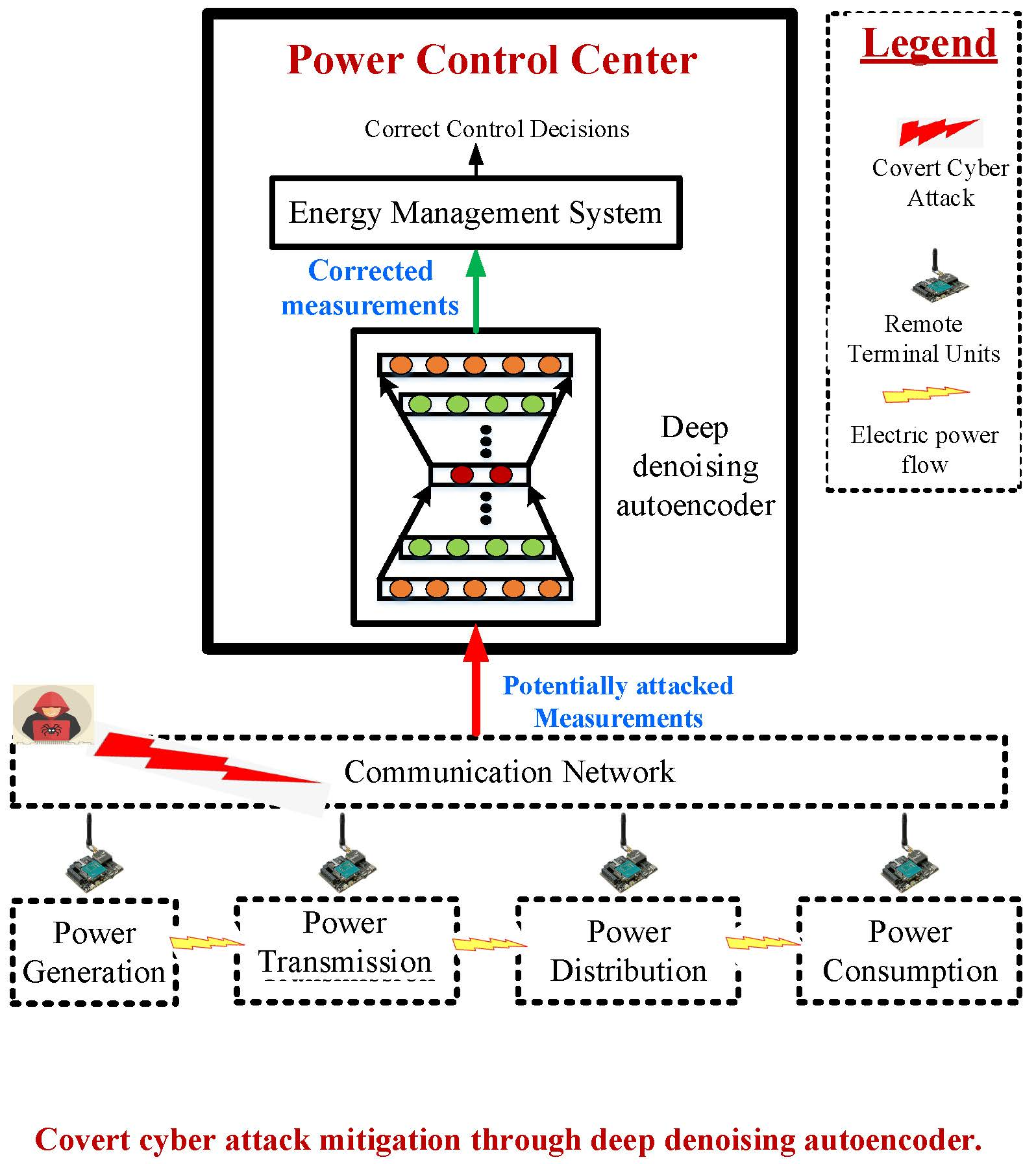
Energies 12 03091 g001
Figure 2. SG Data reconstruction options against CCDA attacks.
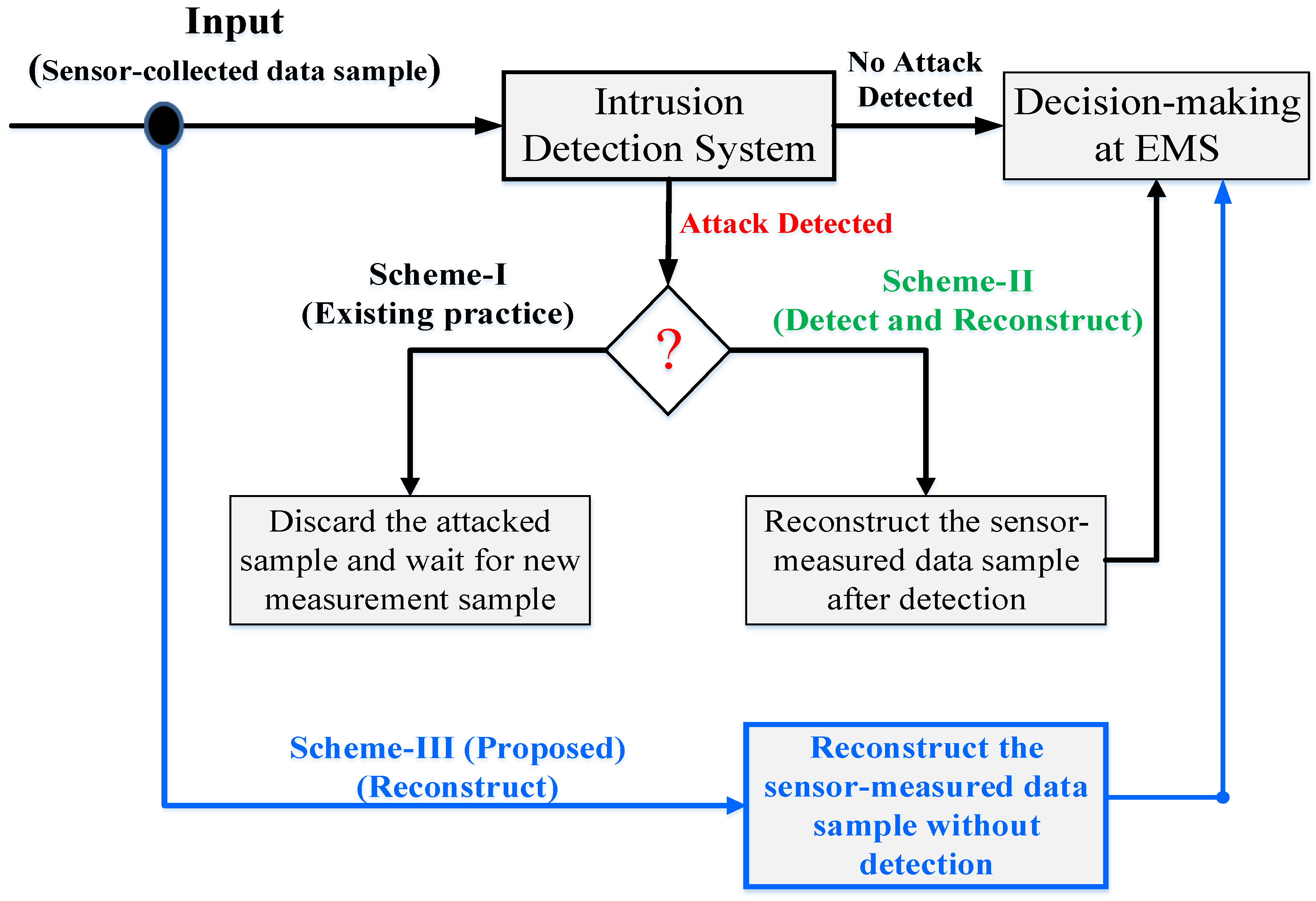
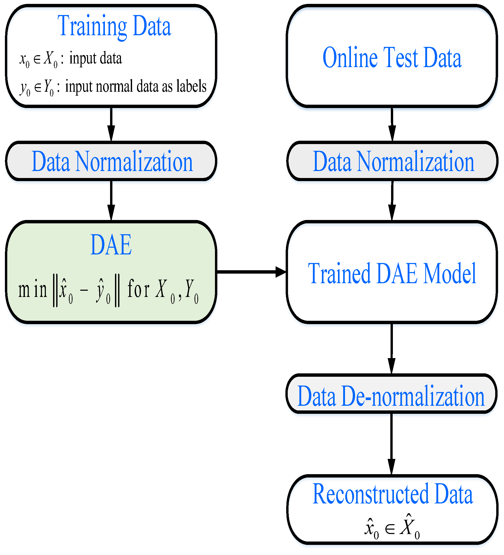
Energies 12 03091 g002
Figure 3. A flowchart of the proposed scheme for reconstruction of data affected by CCDA.
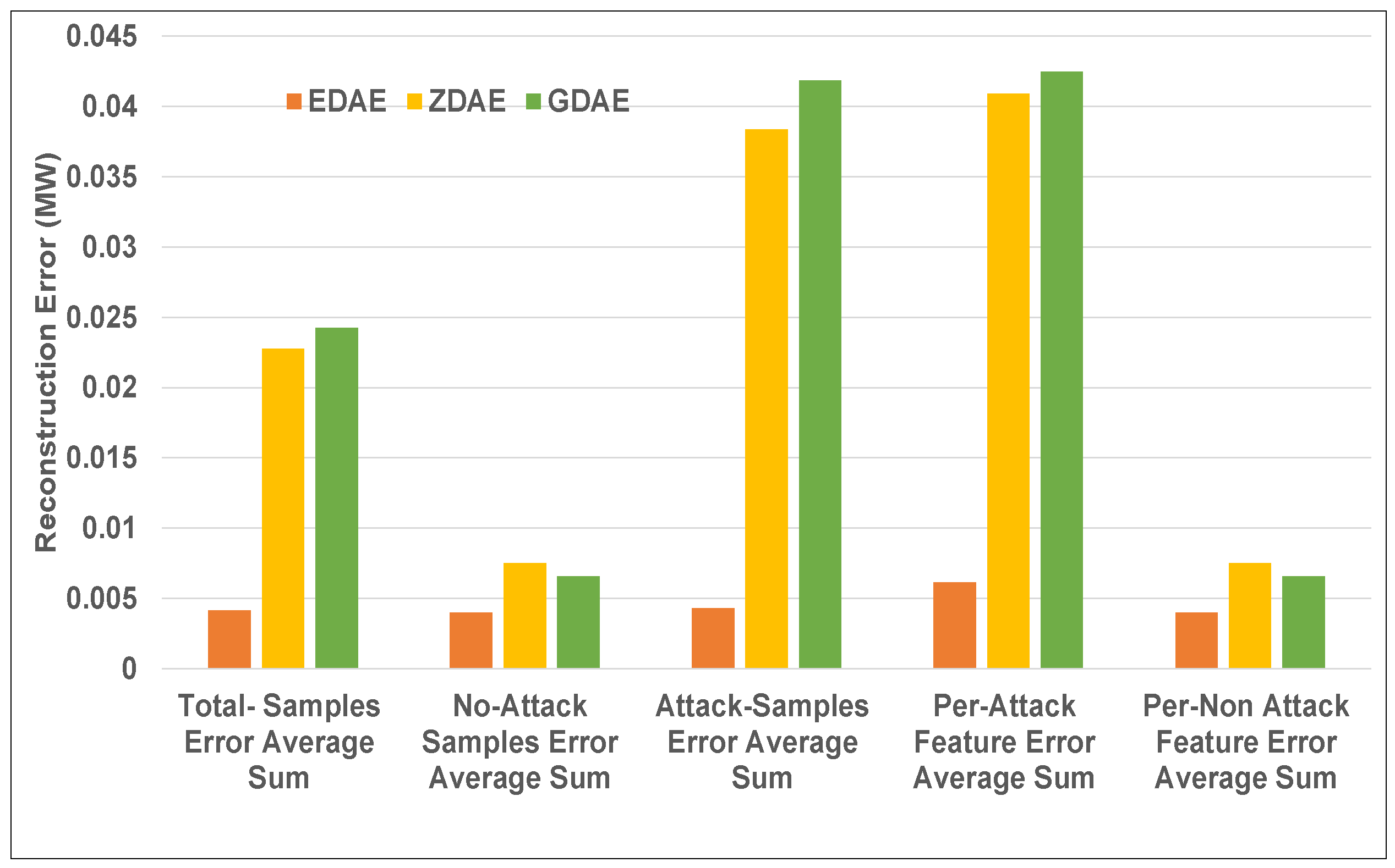
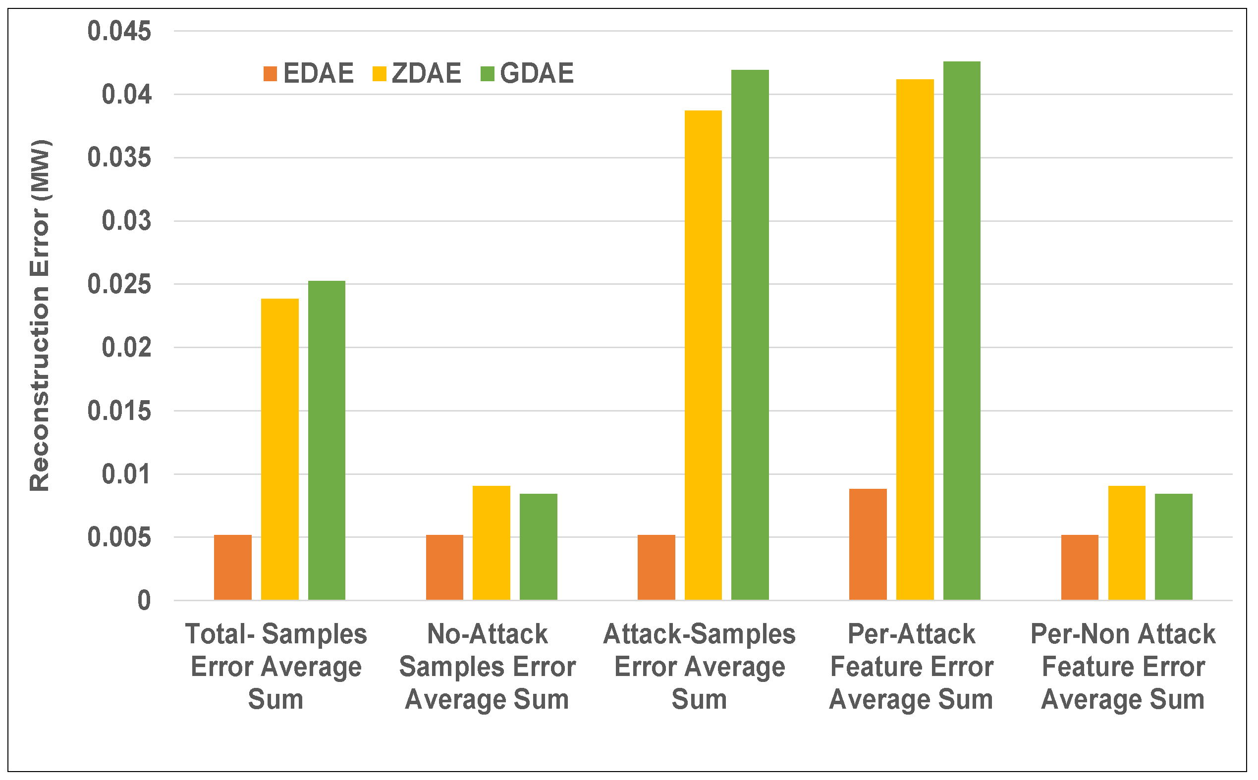
Energies 12 03091 g003
Figure 4. Error average sum for various DAE schemes in a standard IEEE 14-bus system from a 20% fixed-attack dataset.
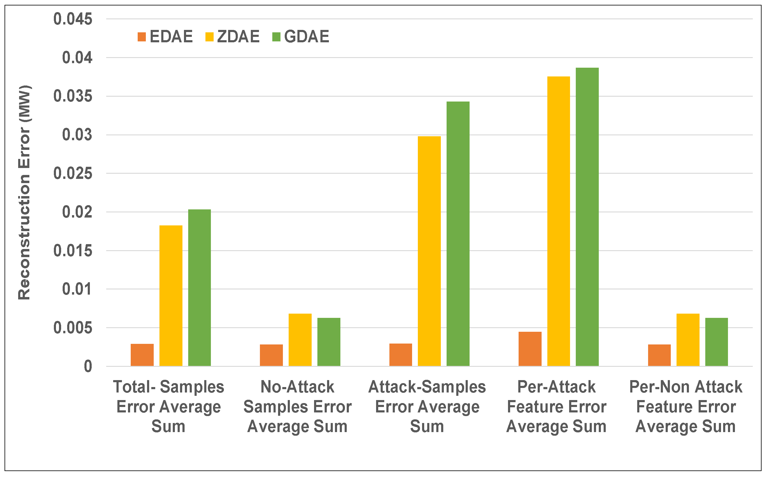
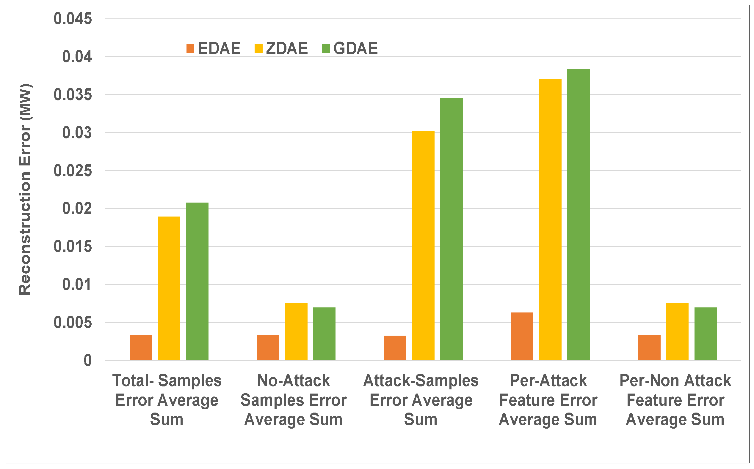
Energies 12 03091 g004
Figure 5. Error average sum for various DAE schemes in a standard IEEE 14-bus system from a 40% fixed-attack dataset.
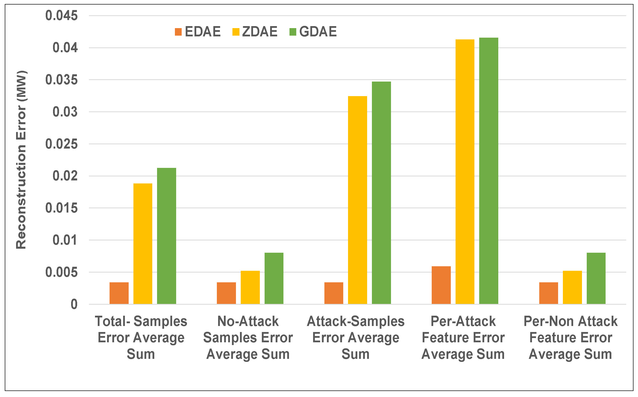
Energies 12 03091 g005
Figure 6. Error average sum for various DAE schemes in a standard IEEE 39-bus system from a 20% fixed-attack dataset.
Energies 12 03091 g006
Figure 7. Error average sum for various DAE schemes in a standard IEEE 39-bus system from a 40% fixed-attack dataset.
Energies 12 03091 g007
Figure 8. Error average sum for various DAE schemes in a standard IEEE 14-bus system from a 20% random-attack dataset.
Energies 12 03091 g008
Figure 9. Error average sum for various DAE schemes in a standard IEEE 14-bus system from a 40% random-attack dataset.
Energies 12 03091 g009
Figure 10. Error average sum for various DAE schemes in a standard IEEE 39-bus system from a 20% random-attack dataset.
Energies 12 03091 g010
Figure 11. Error average sum for various DAE schemes in a standard IEEE 39-bus system from a 40% random-attack dataset.
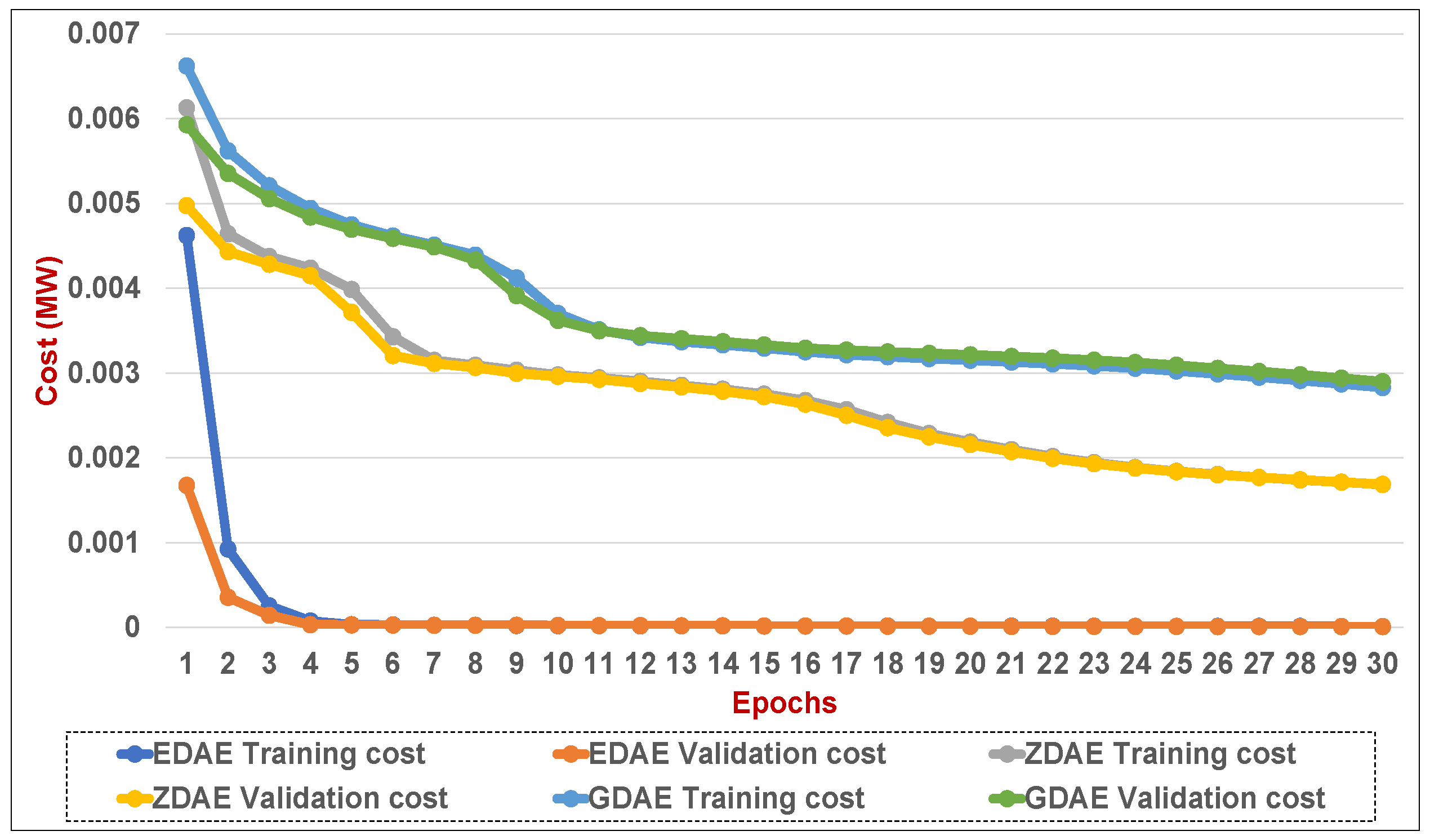
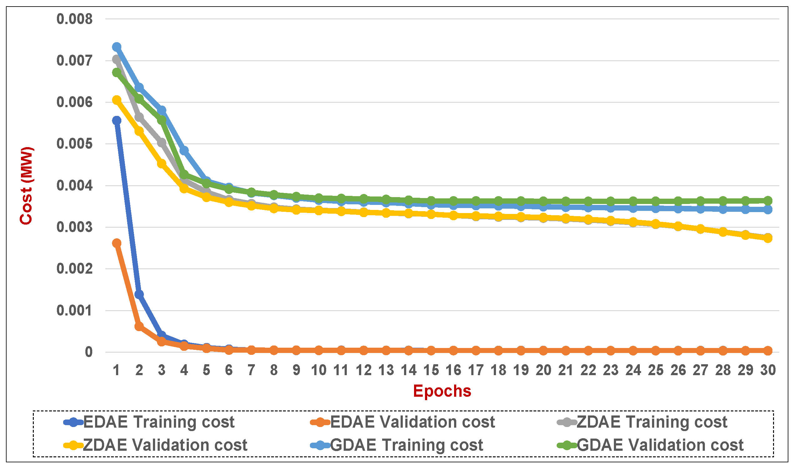
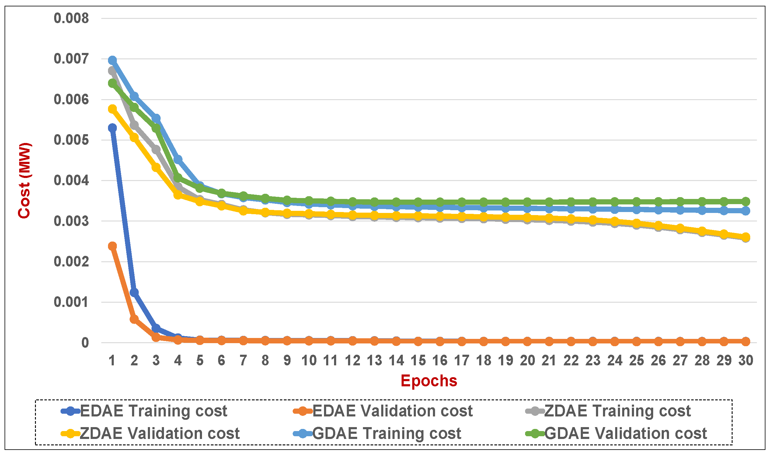
Energies 12 03091 g011
Figure 12. Training and validation costs for various DAE corruption-addition schemes (20% of the features in a fixed attack) in a standard IEEE 14-bus system.
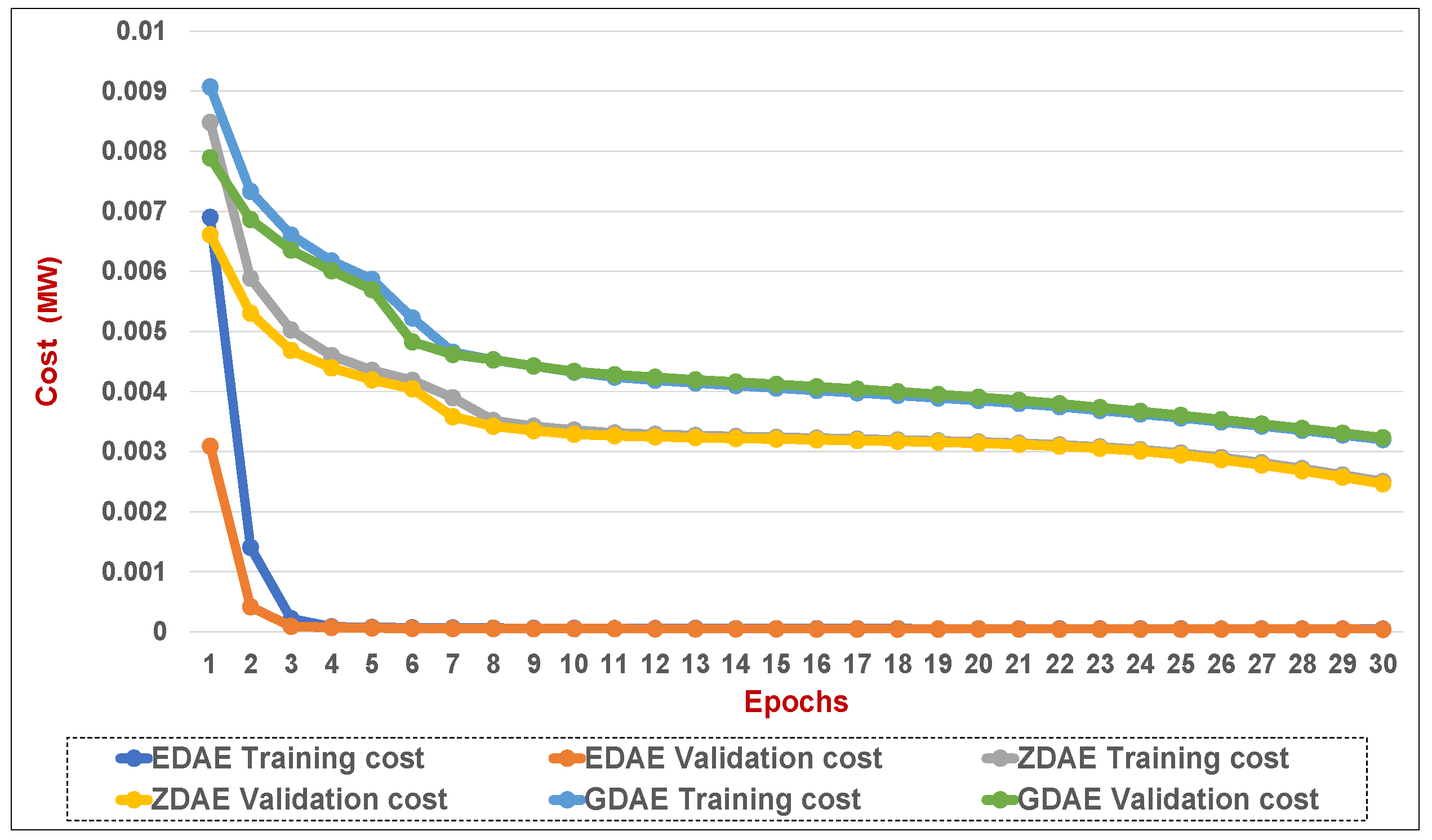
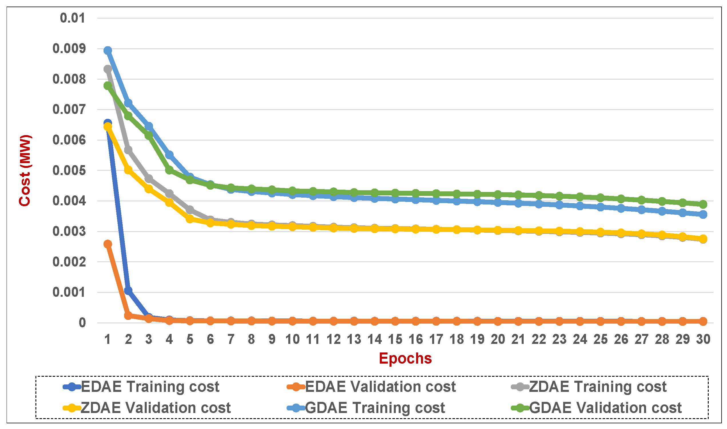
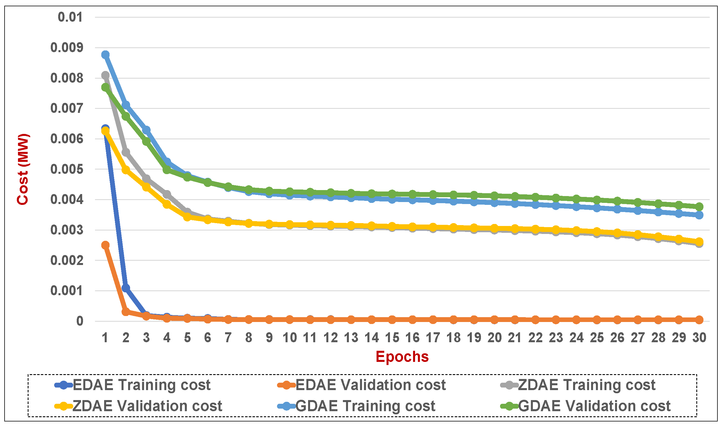
Energies 12 03091 g012
Figure 13. Training and validation costs for various DAE corruption-addition schemes (40% of the features in a fixed attack) in a standard IEEE 14-bus system.
Energies 12 03091 g013
Figure 14. Training and validation costs for various DAE corruption-addition schemes (20% of the features in a fixed attack) in a standard IEEE 39-bus system.
Energies 12 03091 g014
Figure 15. Training and validation costs for various DAE corruption-addition schemes (40% of the features in a fixed attack) in a standard IEEE 39-bus system.
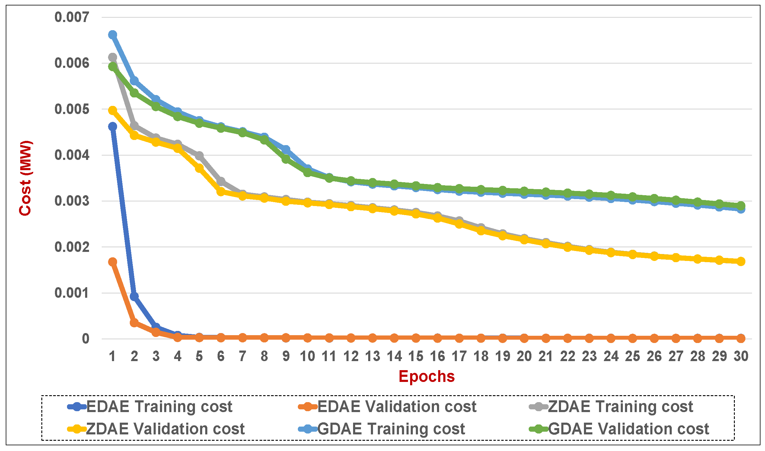
Energies 12 03091 g015
Figure 16. Training and validation costs for various DAE corruption-addition schemes (20% of the features in a random attack) in a standard IEEE 14-bus system.
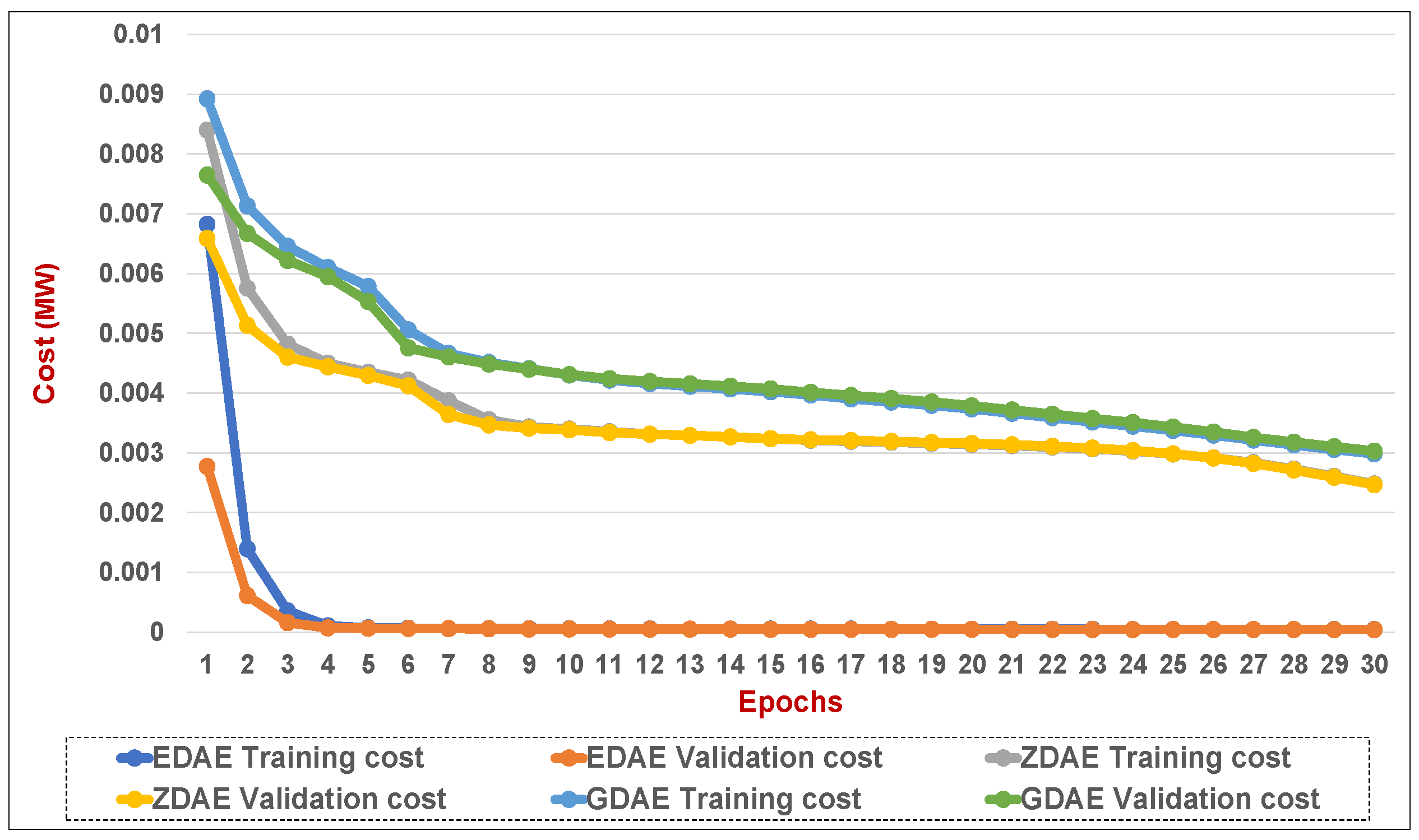
Energies 12 03091 g016
Figure 17. Training and validation costs for various DAE corruption-addition schemes (40% of the features in a random attack) in a standard IEEE 14-bus system.
Energies 12 03091 g017
Figure 18. Training and validation costs for various DAE corruption-addition schemes (20% of the features in a random attack) in a standard IEEE 39-bus system.
Energies 12 03091 g018
Figure 19. Training and validation costs for various DAE corruption-addition schemes (40% of the features in a random attack) in a standard IEEE 39-bus system.
Energies 12 03091 g019
Table 1. A summary of research works on the detection and mitigation tier of defense mechanism in SGs.
Defense TierApplication Area
Detection Tier
(Intrusion detection system (IDS) without utilizing machine learning)
Model-based techniques and game-theoretic methods for security [8,9]EMS
Physical watermarking of control inputs [10]PCC
Integration of run-time semantic analysis with efficient look-ahead PF analysis [11]SCADA
Model-based IDS system to tackle attacks on auto generation control [12]EMS
Integration of host-, and network-based IDS substations [13]SCADA
Generic use of phasor measurement units (PMU) data considering white-list behavior and network topology [14]PMU
IDS to detect PMU data assaulted by the GPS spoofing [15]PMU
Detection of CP assaults on advanced metering network (AMI) systems based on behavior rules [16]AMI
Distributed multi-layered IDS and early warning system [17,18]AMI
Stealth attack identification with cumulative sum and quickest detection [19]EMS and PCC
Abnormal energy consumption detection in smart meters using heuristic methods and contextual analysis of data [20,21,22]Smart meters
Detection Tier
(Intrusion detection system (IDS) utilizing machine learning)
Utilizing machine learning methods for CCDA detection [23,24]PCC/ EMS
Feature selection and supervised learning-based CCDA detection [25,26]PCC
feature extraction and unsupervised learning-based CCDA detection [6]PCC
Identification of CCDA utilizing joint transformation and Kullback–Leibler distance [27]PCC
Deep learning-based recognition of the behavior features for CCDA [28]PCC
Mitigation Tier
(Restoration mechanism to eliminate impacts of attack)
Game theroy-based mitigation (attacker-defender, zero-sum) game [29,30] and zero-sum Markov game-based mitigation [31]Substation
Physical watermarking of control inputs [10]Substation
Integration of run-time semantic analysis with efficient look-ahead PF analysis [11]Substation
Table 2. Possible options for mitigating attacks.
Detect and Discard (Scheme-I)Detect and Reconstruct (Scheme-II)Reconstruct (Scheme-III)
- Attacked samples are dropped- Attacked samples are reconstructed- Reconstruct without detection
- Wait for normal samples to be received- Requires detection and reconstruction time- Requires reconstruction time
Table 3. Advantages of the denoising autoencoder over principal component analysis.
Denoising AutoencoderPrincipal Component Analysis
The DAE can learn nonlinear and linear correlations in the multivariate sensor-collected data from the power grid [34,35,37,38]PCA requires linear and Gaussian assumption about the data [34].
The DAE does not need dictionary elements to be orthogonal, making it adaptable to fluctuations in the representation of data. Thus signal reconstruction capability is improved [34,36,39].PCA reduces the data frame by orthogonally transforming the data into a set of principal components. This limits the performance of PCA in reconstruction of data [34].
By restricting removed variables to be rebuilt from the remaining data, the DAE learns to convolute variables that tend to be correlated. This enhances robustness against noise and local fluctuations in the primary multivariate measurement data [36,39].Reconstruction of noisy or corrupted nonlinear data is much too lossy as compared to PCA [34,35].
Table 4. Dimension growth with increasing sizes of power systems.
SystemStatesDAE Nodes
(Input and Output)
IEEE 14-bus1353
IEEE 39-bus38130
IEEE 57-bus56216
IEEE 118-bus117489
Table 5. Simulation parameters for DAE model.
SystemIEEE
14-Bus
IEEE
39-Bus
IEEE
57-Bus
IEEE
118-Bus
Input and Output Nodes531301353
DAE Layers3222
Code Layer size3475140318
Total Data200,000200,000200,000200,000
Training Data100,000100,000100,000100,000
Test Data100,000100,000100,000100,000
OptimizerMSEMSEMSEMSE
NormalizationMin-MaxMin-MaxMin-MaxMin-Max
Batch Size1111
Epochs30303030
Table 6. Seven best-reconstructed features (20% fixed-attack on 20% of the features in a standard IEEE 14-bus system) with the EDAE scheme.
Feature Number19473846492418
Feature Value−24.31−0.10896−42−17.574−6.86498.0950.4
Reconstructed Value−2.43 × 101−1.09 × 10⁻¹−4.20 × 101−1.76 × 101−6.86 × 1008.09 × 1005.04 × 101
Error5.88 × 10 6 1.39 × 10 5 5.18 × 10 5 6.14 × 10 5 6.47 × 10 5 8.01 × 10 5 0.00010462
Error Ratio8.50 × 10 8 3.84 × 10 6 6.75 × 10 7 7.19 × 10 6 1.12 × 10 6 4.24 × 10 6 6.09 × 10 6
Table 7. Seven worst-reconstructed features( fixed attack on 20% of the features in a standard IEEE 14-bus system) with the EDAE scheme.
Feature Number33819134450
Feature Value5.2503−35.86216.015−10.707−15.029−6.7417−11.735
Reconstructed Value5.25731468−35.8580567216.01861077−10.70396887−15.02630777−6.739086843−11.73276872
Error5.25731468−35.8580567216.01861077−10.70396887−15.02630777−6.739086843−11.73276872
Error Ratio0.0013360530.0001099570.0002254620.0002830980.0001791350.0003876110.000190139
Table 8. Seven best-reconstructed features (fixed attack on 40% of the features in a standard IEEE 14-bus system) with the EDAE scheme.
Feature Number16241844364338
Feature Value71.2486.778550.363−8.1342−71.248−52.386−41.969
Reconstructed Value7.12 × 10 1 6.78 × 10 0 5.04 × 10 1 −8.13 × 10 0 −7.12 × 10 1 −5.24 × 10 1 −4.20 × 10 1
Error6.05 × 10 6 2.60 × 10 5 3.40 × 10 5 5.84 × 10 5 7.95 × 10 5 0.0002218830.000255396
Error Ratio8.50 × 10 8 3.84 × 10 6 6.75 × 10 7 7.19 × 10 6 1.12 × 10 6 4.24 × 10 6 6.09 × 10 6
Table 9. Seven worst-reconstructed features (fixed attack on 40% of the features in a standard IEEE 14-bus system) with the EDAE scheme.
Feature Number4287132335
Feature Value−9.310228.447−0.21257−15.038−114.815.2384−11.576
Reconstructed Value−9.30542371928.45157074−0.208140482−15.03418581−114.8066195.241757108−11.57308739
Error0.0047762810.0045707440.0044295180.0038141950.0033810420.0033571080.002912608
Error Ratio0.0005130160.0001606760.0208379260.0002536372.9449 × 10 5 0.0006408650.000251607
Table 10. Seven best-reconstructed features (fixed attack on 20% of the features in a standard IEEE 14-bus system) with the ZDAE scheme.
Feature Number2149294193515
Feature Value29.115−5.7354−5.7354−29.115−10.608−73.44373.443
Reconstructed Value29.11551588−5.73057252−5.729508174−29.10641015−10.59362174−73.4270163973.46094698
Error0.000515880.004827480.0058918260.0085898510.014378260.0159836060.017946978
Error Ratio1.77187 × 10 5 0.0008416990.0010272740.0002950320.0013554170.0002176330.000244366
Table 11. Seven worst-reconstructed features (fixed attack on 20% of the features in a standard IEEE 14-bus system) with the ZDAE scheme.
Feature Number22424151217
Feature Value16.856−20.227−9.310216.01−11.576−13.83456.302
Reconstructed Value17.3320005−19.75872138−9.01586187716.29326843−11.40118695−13.6673870356.46786937
Error0.4760005010.4682786210.2943381230.2832684280.1748130470.1666129740.165869371
Error Ratio0.0282392320.0231511650.0316145870.0176932180.0151013340.0120437310.002946065
Table 12. Seven best-reconstructed features (fixed attack on 40% of the features in a standard IEEE 14-bus system) with the ZDAE scheme.
Feature Number3993515325219
Feature Value24.31−10.707−73.4788.1641.7611−1.4676−24.31
Reconstructed Value2.43 × 10 1 −1.07 × 10 1 −7.35 × 10 1 8.82 × 10 1 1.77 × 10 0 −1.45 × 10 0 −2.43 × 10 1
Error9.29 × 10 5 0.0039139560.0092653810.0096738240.0108494090.0135018050.021025564
Error Ratio3.82 × 10 6 3.66 × 10 4 1.26 × 10 4 1.10 × 10 4 6.16 × 10 3 9.20 × 10 3 8.65 × 10 4
Table 13. Seven worst-reconstructed features (fixed attack on 40% of the features in a standard IEEE 14-bus system) with the ZDAE scheme.
Feature Number224211171148
Feature Value16.855−20.226−6.33556.34616.015153.52−35.862
Reconstructed Value17.2521351−19.8600899−5.97621665556.675706916.30432973153.773394−35.6177516
Error0.3971350990.3659100950.3587833450.3297068980.2893297310.2533939630.244248405
Error Ratio3.82 × 10 6 3.66 × 10 4 1.26 × 10 4 1.10 × 10 4 6.16 × 10 3 9.20 × 10 3 8.65 × 10 4
Table 14. Seven best-reconstructed features (fixed attack on 20% of the features in a standard IEEE 14-bus system) with the GDAE scheme.
Feature Number23384712271825
Feature Value6.778524.427−28.447−15.03828.447−24.42717.551
Reconstructed Value6.78 × 10 0 2.44 × 10 1 −2.84 × 10 1 −1.50 × 10 1 2.84 × 10 1 −2.44 × 10 1 1.76 × 10 1
Error2.40 × 10 5 0.0001351490.0002416910.0003304280.0006857050.0007730760.001103067
Error Ratio3.55 × 10 6 5.53 × 10 6 8.50 × 10 6 2.20 × 10 5 2.41 × 10 5 3.16 × 10 5 6.28 × 10 5
Table 15. Seven worst-reconstructed features (fixed attack on 20% of the features in a standard IEEE 14-bus system) with the GDAE scheme.
Feature Number310728483151
Feature Value−9.3102−6.2287−29.7675.7354−5.73541.5209−1.5209
Reconstructed Value−9.271860897−6.190712099−29.737004565.75936093−5.7117314961.543764792−1.498413224
Error0.0383391030.0379879010.029995440.023960930.0236685040.0228647920.022486776
Error Ratio0.0041179680.0060988490.0010076740.0041777260.004126740.0150337250.014785177
Table 16. Seven best-reconstructed features (fixed attack on 40% of the features in a standard IEEE 14-bus system) with the GDAE scheme.
Feature Number482237281716
Feature Value−5.735443.655−41.9695.735441.969−95.675−0.21257
Reconstructed Value−5.73478155843.6563242−41.9669895.73871376541.97239975−95.67142491−0.207780056
Error0.1598769430.1450200780.131724840.1311273640.104959390.0866725870.083504682
Error Ratio−0.0001078293.03333 × 10 5 −4.79163 × 10 5 0.0005777748.10061 × 10 5 −3.73671 × 10 5 −0.022533488
Table 17. Seven worst-reconstructed features (fixed attack on 40% of the features in a standard IEEE 14-bus system) with the GDAE scheme.
Feature Number4113333711
Feature Value−5.735443.655−41.9695.735441.969−95.675−0.21257
Reconstructed Value−5.73478155843.6563242−41.9669895.73871376541.97239975−95.67142491−0.207780056
Error0.0006184420.0013242010.0020109980.0033137650.0033997460.0035750930.004789944
Error Ratio0.0001078293.03333 × 10 5 4.79163 × 10 5 0.0005777748.10061 × 10 5 3.73671 × 10 5 0.022533488
Table 18. Seven best-reconstructed features (random attack on 20% of the features in a standard IEEE 14-bus system) with the EDAE scheme.
Feature Number25412450215215
Feature Value1.76 × 10 1 −1.69 × 10 1 7.73 × 10 0 2.99 × 10 0 1.69 × 10 1 −5.27 × 10 0 7.36 × 10 1
Reconstructed Value1.76 × 10 1 −1.69 × 10 1 7.73 × 10 0 2.99 × 10 0 1.69 × 10 1 −5.27 × 10 0 7.36 × 10 1
Error2.42 × 10 5 3.72 × 10 5 0.0001219650.0001456020.0002262260.0002325320.000244578
Error Ratio1.38 × 10 6 2.20 × 10 6 1.58 × 10 5 4.88 × 10 5 1.34 × 10 5 4.41 × 10 5 3.33 × 10 6
Table 19. Seven worst-reconstructed features (random attack on 20% of the features in a standard IEEE 14-bus system) with the EDAE scheme.
Feature Number49814381845
Feature Value−9.9661−8.6655−95.556−11.794−42.103−24.313−7.734
Reconstructed Value−9.960711568−8.660489164−95.55141419−11.78952318−42.09859985−24.3087889−7.730274573
Error0.0053884320.0050108360.004585810.0044768240.0044001520.0042110970.003725427
Error Ratio0.0005406760.0005782514.79908 × 10 5 0.0003795850.0001045090.0001732030.000481695
Table 20. Seven best-reconstructed features (random attack on 40% of the features in a standard IEEE 14-bus system) with the EDAE scheme.
Feature Number20352932434014
Feature Value29.111−73.5545.67985.2682−6.7198−29.11173.554
Reconstructed Value2.91 × 10 1 −7.36 × 10 1 5.68 × 10 0 5.27 × 10 0 −6.72 × 10 0 −2.91 × 10 1 7.36 × 10 1
Error4.64 × 10 5 5.41 × 10 5 6.26 × 10 5 0.0002242460.0004065350.0004908510.000534421
Error Ratio1.59 × 10 6 7.36 × 10 7 1.10 × 10 5 4.26 × 10 5 6.05 × 10 5 1.69 × 10 5 7.27 × 10 6
Table 21. Seven worst-reconstructed features (random attack on 40% of the features in a standard IEEE 14-bus system) with the EDAE scheme.
Feature Number7114744991
Feature Value0.046326−13.885−28.613−11.794−9.9661−3.734−95.556
Reconstructed Value0.05920957−13.87618859−28.60460809−11.78692803−9.959870581−3.728092846−95.55035503
Error0.012883570.0088114120.0083919090.0070719680.0062294190.0059071540.005644974
Error Ratio0.278106670.0006345990.000293290.0005996240.0006250610.0015819915.9075 × 10 5
Table 22. Seven best-reconstructed features (random attack on 20% of the features in a standard IEEE 14-bus system) with the ZDAE scheme.
Feature Number41142144422449
Feature Value−16.88873.55416.888−7.734−43.8367.734−9.9661
Reconstructed Value−16.8865953673.5557495716.88984495−7.732058335−43.834051517.736052894−9.963812929
Error0.0014046360.0017495670.0018449530.0019416650.001948490.0020528940.002287071
Error Ratio8.31736 × 10 5 2.37862 × 10 5 0.0001092460.0002510564.44496 × 10 5 0.0002654380.000229485
Table 23. Seven worst-reconstructed features (random attack on 20% of the features in a standard IEEE 14-bus system) with the ZDAE scheme.
Feature Number52747721140
Feature Value−0.5438−0.046326−29.855−48.433−6.169−29.11129.111
Reconstructed Value−0.4024963850.062047902−29.74962789−48.35341728−6.09788107−29.0439860229.17169563
Error0.1413036150.1083739020.1053721070.0795827250.071118930.0670139830.06069563
Error Ratio0.2598448242.3393753450.0035294630.0016431510.0115284370.0023020160.002084972
Table 24. Seven best-reconstructed features (random attack on 40% of the features in a standard IEEE 14-bus system) with the ZDAE scheme.
Feature Number42221814384424
Feature Value−43.83616.888−24.31373.55424.313−7.7347.734
Reconstructed Value−43.8357859816.88835338−24.3109117373.556166124.31673587−7.7294020897.739212442
Error0.0002140250.0003533780.0020882710.0021660960.0037358690.0045979110.005212442
Error Ratio4.88239 × 10 6 2.09248 × 10 5 8.58911 × 10 5 2.94491 × 10 5 0.0001536570.0005945060.000673965
Table 25. Seven worst-reconstructed features (random attack on 40% of the features in a standard IEEE 14-bus system) with the ZDAE scheme.
Feature Number12197473352
Feature Value−15.23416.22−3.734−29.8556.71985.2682−1.565
Reconstructed Value−15.1436023516.30842128−3.673237667−29.805707946.7649579185.312002445−1.523176287
Error0.0903976480.0884212840.0607623330.0492920570.0451579180.0438024450.041823713
Error Ratio0.005933940.0054513740.0162727190.0016510490.0067201280.0083144990.026724418
Table 26. Seven best-reconstructed features (random attack on 20% of the features in a standard IEEE 14-bus system) with the GDAE scheme.
Feature Number1241212024304
Feature Value−13.885−29.11116.88829.1116.71989.9661−11.794
Reconstructed Value−13.88377492−29.1095701716.8896596929.112748246.7216329539.967963504−11.79191121
Error0.0012250770.0014298320.0016596870.0017482390.0018329530.0018635040.002088788
Error Ratio8.82302 × 10 5 4.91165 × 10 5 9.82761 × 10 5 6.00542 × 10 5 0.0002727690.0001869840.000177106
Table 27. Seven worst-reconstructed features (random attack on 20% of the features in a standard IEEE 14-bus system) with the GDAE scheme.
Feature Number1733130218
Feature Value−95.556−95.556−153.53153.5316.22−95.556−24.313
Reconstructed Value−95.48854845−95.49835622−153.4731469153.585980116.27401379−95.50443633−24.27054722
Error0.0674515530.0576437750.0568531030.0559801480.0540137950.0515636690.042452777
Error Ratio0.0007058850.0006032460.0003703060.000364620.0033300740.0005396170.001746094
Table 28. Seven best-reconstructed features (random attack on 40% of the features in a standard IEEE 14-bus system) with the GDAE scheme.
Feature Number14422213331938
Feature Value73.554-43.83643.836153.53−153.5342.103−42.103
Reconstructed Value73.55511276−43.8336646343.83835556153.5325412−153.525855142.10726753−42.09863462
Error0.0011127640.0023353710.0023555630.002541210.0041449260.0042675310.004365384
Error Ratio1.51285 × 10 5 5.32752 × 10 5 5.37358 × 10 5 1.65519 × 10 5 2.69975 × 10 5 0.0001013590.000103683
Table 29. Seven worst-reconstructed features (random attack on 40% of the features in a standard IEEE 14-bus system) with the GDAE scheme.
Feature Number2117128019
Feature Value−48.433−13.885−95.556−13.885−8.665516.22−62.336
Reconstructed Value−48.30994115−13.79823827−95.47778432−13.80909392−8.59167469616.2896147−62.26993855
Error0.1230588540.0867617320.0782156810.0759060780.0738253040.0696146990.066061451
Error Ratio0.0025408060.0062485940.0008185320.0054667680.0085194510.0042919050.001059764

