Condition Monitoring for the Roller Bearings of Wind Turbines under Variable Working Conditions Based on the Fisher Score and Permutation Entropy

Abstract

Condition monitoring is used to assess the reliability and equipment efficiency of wind turbines. Feature extraction is an essential preprocessing step to achieve a high level of performance in condition monitoring. However, the fluctuating conditions of wind turbines usually cause sudden variations in the monitored features, which may lead to an inaccurate prediction and maintenance schedule. In this scenario, this article proposed a novel methodology to detect the multiple levels of faults of rolling bearings in variable operating conditions. First, signal decomposition was carried out by variational mode decomposition (VMD). Second, the statistical features were calculated and extracted in the time domain. Meanwhile, a permutation entropy analysis was conducted to estimate the complexity of the vibrational signal in the time series. Next, feature selection techniques were applied to achieve improved identification accuracy and reduce the computational burden. Finally, the ranked feature vectors were fed into machine learning algorithms for the classification of the bearing defect status. In particular, the proposed method was performed over a wide range of working regions to simulate the operational conditions of wind turbines. Comprehensive experimental investigations were employed to evaluate the performance and effectiveness of the proposed method.

1. Introduction

In the non-fossil policy of modern society, wind energy has become one of the most promising renewable energy sources due to low CO₂ emissions during its entire lifespan, which makes a wind farm a very reliable and efficient choice in windy sites [1,2,3]. Besides the visual aspects, it is noted that the noise impact may represent a major hindrance to new wind farms [4,5]. Considering the noise pollution and the wind energy utilization, wind turbines are usually installed in complex territory like hills or mountains under very harsh environmental conditions [6], and they suffer from changing weather, temperature, random wind speed, wind shear effect, tower shadow effect and severe loads. Moreover, the wind shear and tower shadow effect play a key role in reducing the accuracy of predicting wind speed, which makes wind turbines operate under fluctuating conditions [7]. All these adverse factors cause wind turbines to encounter failure. To face the challenges associated with wind turbine failure, condition monitoring has developed rapidly to increase the availability and reduce the operations and maintenance costs of wind turbines [8]. Condition monitoring involves sensors and signal processing equipment to identify the changes in the wind turbine components, predict early faults and schedule the condition-based maintenance in time. The common approaches for the condition monitoring of wind turbines include vibration analysis, acoustics, oil analysis, strain measurement, and thermography [9].

There are many studies focused on condition monitoring and relevant technological innovations. As vibration analysis is still the most popular approach, many studies have contributed to signal-processing methods for condition monitoring, such as the short-time Fourier transform (STFT), Wigner–Ville distribution (WVD) [10,11] and wavelet transform (WT) [12,13]. Alternatively, the S-transform is superior in the time-frequency analyses of non-stationary signals, which eliminates the limitations of STFT and WT [14]. Moreover, the empirical mode decomposition (EMD) method shows excellent performance in non-stationary signal processing due to its local adaptive feature [15,16]. Nevertheless, the EMD also has some limits in application due to its recursive calculation and mode-mixing problems [17,18]. To overcome the drawbacks of the EMD method, variational mode decomposition (VMD) has been proposed by decomposing a multicomponent signal into a set of intrinsic mode functions (IMFs) [19], which has been proven beneficial in signal reconstruction and noise reduction [20]. Among the prior literature, the analysis techniques based on vibration data [21,22] have been widely used for condition monitoring. In Ref. [23], the data analyses for condition monitoring include conventional statistical analyses, trend estimation, physical modeling analyses and machine learning. However, the Supervisory Control and Data Acquisition (SCADA) data analysis yields false alarms [24,25] frequently due to the low sampling rate and noisy training data. Additionally, the monitoring data vary over a wide range with the random operational conditions and the weather environment, challenging the model accuracy of condition monitoring systems [22].

Alternatively, some effort has been invested in data preprocessing to normalize the operational variability. Refs. [26,27] incorporate the temperature of the gearbox as a reference parameter to evaluate the health status of wind turbines. By building the energy balance model, the efficiency loss of the turbine output power could be calculated to deliver the fault information. However, the environmental temperature varied with the changes in season and affected the accuracy of the proposed method. To normalize the variable monitoring data, many studies have proposed using a statistical parameter as the indicator feature, such as the average root mean square (RMS) amplitude, extreme value, average deviation, skewness, kurtosis, shape factor, and cross zero rate [28].

Along with what was discussed above, the selection of the statistical parameter also needs to be taken seriously because the features that carry useful information are beneficial for increasing the computational efficiency and the fault detection accuracy. Many feature selection criteria have been proposed to improve the performance of identification systems. The Wilcoxon rank sum and information gain were adopted and compared in the classification of muscle fatigue using surface electromyography signals [29]. In Ref. [30], the Laplacian score (LS) is adopted to refine the fault features that were extracted from the planetary gearboxes under non-stationary working conditions. The selected features were trained in a least square support vector machine. In Ref. [31], considering the high dimensionality of the extracted original feature, the ReliefF algorithm is used to select optimal features to optimize the support vector machine (SVM) performance. Additionally, genetic algorithms (GAs) have been used to select the input features and the characteristic parameters of the classifiers for bearing fault detection. In general, feature ranking is widely utilized in condition monitoring and fault diagnosis to enhance the accuracy of the classification result and ease the computational burden.

In this article, an alternative methodology for the condition monitoring of roller bearings is proposed to investigate the effectiveness of multifeature fusion under the varying operating conditions of wind turbines. In particular, the vibration signal was decomposed to a set of intrinsic mode functions by VMD. The statistical features of each IMF, which cover the multiscale moments and other commonly used statistical properties of the distribution, are extracted by using the LibXtract library. The Fisher score is adopted to select the effective features. Finally, the selected features are imported into the multi-class classifier. To be specific, the multi-class classifier focuses mainly on multi-class SVM. Meanwhile, an artificial neural network (ANN) is imported as reference for verification. Both the accuracy of the evaluation results and the computational efficiency will be presented. The main contributions of the proposed approach include the following: (1) the bearing detection of CM was performed on a range of fluctuating operating conditions rather than on a certain fixed condition; (2) based on the permutation entropy and Fisher score, the proposed method mitigates the adverse impact of the fluctuating conditions; and (3) experimental investigations were performed to verify the efficiency of the proposed method by presenting the experimental results and the performance analysis.

The remainder of this paper is organized as follows: Section 2 gives a brief review of the theoretical background. Section 3 presents the experimental setup and the proposed method of condition monitoring based on feature extraction, selection and classification. Section 4 presents the experimental description and the analysis, together with the discussion. Finally, the conclusions are presented.

2. Theoretical Background

2.1. Variational Mode Decomposition (VMD)

Variational mode decomposition (VMD) is aimed at decomposing a signal into band-limited subsignals in a non-recursive manner. The decomposed signal, which is also defined as intrinsic mode function (IMF) u_k, has certain sparse properties in the spectrum domain. It is assumed that each subsignal is concentrated around a corresponding center pulsation. Thus, the bandwidth of each mode is chosen by utilizing the H1 Gaussian smoothness for the transformed signal.

To obtain the bandwidth of each mode function, VMD first utilizes the Hilbert transform to convert each mode u_k into an analytic expression u_k⁺ in a single-sided spectral domain as shown in Equation (1), where δ(t) is the unit impulse function.

$$u_k^{+}(t)=\left(\delta (t)+\frac{j}{\pi t}\right)\times u_k(t)$$

(1)

After the Hilbert transformation, the frequency spectrum of each mode is shifted to the baseband, and the respective estimated center frequency is adjusted by using an exponential tuned term. Then, the bandwidth is estimated through the Gaussian smoothness of the demodulated signal by utilizing the squared L2-norm of the gradient [32]. Thus, the VMD process is realized by solving a constrained variational problem [33]:

$$\underset{\left\{u_k\right\},\left\{{\omega }_k\right\}}{\min }\left\{{\displaystyle \sum _{k=1}^K{\Vert \partial \left[\left(\delta (t)+\frac{j}{\pi t}\right)\times u_k(t)\right]e^{-j{\omega }_{k}t}\Vert }_2^2}\right\},subjectto{\displaystyle \sum _{k=1}^K{u}_k(t)}=f(t)$$

(2)

where f(t) is the target signal, {u_k}: = {u₁, …, u_K} represents the set of the decomposed modes and {ω_k}: = {ω₁, …, ω_K} represents the respective center frequencies. Then, the constraint optimization problem in Equation (2) can be converted into an unconstrained problem via a quadratic penalty term and Lagrangian multipliers as below:

$$ℒ\left(\left\{u_k\right\},\left\{{\omega }_k\right\},\lambda \right)=\alpha {\displaystyle \sum _{k=1}^K{\Vert \partial \left[\left(\delta (t)+\frac{j}{\pi t}\right)\times u_k(t)\right]e^{-j{\omega }_{k}t}\Vert }_2^2}+{\Vert f(t)-{\displaystyle \sum _{k=1}^K{u}_k(t)}\Vert }_2^2+\langle \lambda (t),f(t)-{\displaystyle \sum _{k=1}^K{u}_k(t)}\rangle$$

(3)

To solve the original minimization problem, the alternate direction method of multipliers (ADMM) is adopted to determine the saddle point of the augmented Lagrangian in a sequence of iterative suboptimizations. The details of the VMD algorithm are summarized in [19]. By this process, all the mode functions are obtained and updated by Wiener filtering to tune the center frequency in the spectral domain:

$$\begin{array}{l}{\widehat{u}}_k^{n+1}(\omega )=\frac{\widehat{f}(\omega )-{\displaystyle {\sum }_{i<k}{\widehat{u}}_i^{n+1}(\omega )}-{\displaystyle {\sum }_{i>k}{\widehat{u}}_i^n(\omega )}+\frac{{\widehat{\lambda }}^n(\omega )}{2}}{1+2\alpha {(\omega -{\omega }_k^n)}^2}(\omega >0)\\ {\omega }_k^{n+1}=\frac{{\displaystyle {\int }_0^{\infty }\omega {\left|{\widehat{u}}_k^{n+1}(\omega )\right|}^{2}d\omega }}{{\displaystyle {\int }_0^{\infty }{\left|{\widehat{u}}_k^{n+1}(\omega )\right|}^{2}d\omega }}\end{array}$$

(4)

The center frequency ω_kⁿ is calculated from the weighted center of each mode in the spectral domain. This means that the center represents the frequency for the least squares linear regression of the instantaneous phase. The VMD algorithm is presented in

Table 1. The variational mode decomposition (VMD) algorithm steps.

	Complete VMD Optimization
Step 1:	Initialize $\left\{{\widehat{u}}_k^1\right\}$ , $\left\{{\omega }_k^1\right\}$
Step 2:	${\widehat{\lambda }}^1$, n, set values to 0
Step 3:	Update ${\widehat{u}}_k^{}$and ${\omega }_k^{}$, based on Equation (4)
Step 4:	Update ${\widehat{\lambda }}^{n+1}(\omega )={\widehat{\lambda }}^n(\omega )+\tau \left(\widehat{f}(\omega )-{\displaystyle \sum _k{\widehat{u}}_k^{n+1}(\omega )}\right)$
Step 5:	Check ${{\displaystyle {\sum }_k\Vert {\widehat{u}}_k^{n+1}-{\widehat{u}}_k^n\Vert }}_2^2/{\Vert {\widehat{u}}_k^n\Vert }_2^2<\epsilon$ Repeat Steps 3 and 4 until the convergence condition is met
Step 6:	End the decomposition

as well as Appendix A.

2.2. Information Entropy

In the field of information theory, entropy is a conventional approach to indicate the degree of uncertainty in a random system. Since the entropy increases with the degree of randomness for an observed system, it could be utilized in a quantitative analysis for feature extraction in the field of condition monitoring. Different entropy analysis has been studied and presented including Shannon entropy, Renyi entropy, tsallis entropy, sample entropy and permutation entropy. Renyi entropy was defined as an entropy of order α by Renyi [34]. The application of the Renyi entropy can be found in many areas such as mathematical statistics, signal processing and economics. Another entropy, permutation entropy, exhibits distinctive advantages in retaining the original information of time series [35]. Moreover, permutation entropy is able to improve algorithm robustness for classification. Because permutation entropy has more parameters than Renyi entropy, it can obtain data information under different conditions by controlling the change of parameters.

In this paper, Renyi entropy and permutation entropy are chosen as the extracted features for the condition classification. Also, the correlation of different features like entropy and time-domain statistical value would be presented and compared in Section 3.2.

2.2.1. Renyi Entropy

The concept of Renyi entropy has been widely utilized to quantify the diversity, uncertainty and randomness of a system for rotation machines. Consider a time series variable X, where the data length is finite. The probability distribution of X is defined as Px. The Renyi entropy is defined as:

$$RE(X)=\frac{1}{1-\beta }\log \left({\displaystyle \sum _{i=1}^N{p}_i^{\beta }}\right)\left(\beta \ge 0,\beta \ne 1\right)$$

(5)

It can be noted that the selection of the β parameter is vital to the final statistical result of Renyi entropy. The ability to perceive a small probability is reduced as the β parameter increases. Meanwhile, ability to perceive a small probability is strengthened as the β parameter decreases. Thus, the β parameter should be appropriate based on the characteristics of the decomposed IMF. Additionally, when the β parameter is set as 1, the Renyi entropy is transformed into the Shannon entropy.

2.2.2. Permutation Entropy

The permutation entropy is utilized to recognize the health status of rotation machines [36]. By counting the ordinal patterns, the temporal information of the monitored object is recognized by the permutation entropy. Since the Renyi entropy can only measure the degree of uncertainty in the vibration signals in a single time scale, the permutation entropy is able to estimate the time-series complexity after comparing the neighboring values. By definition, the permutation entropy is calculated by the time-series probability density function based on the Shannon entropy. For a time domain series with a finite length of N, {x(t)} (t = 1, 2,…, N), a segment can be constructed by an m-order dimension. Each m-order segment is then sorted in an ascending sequence that is defined as permutation pattern π. Considering the time delay α, the m-order segment X is defined as follows:

$$X_i^m=\left\{x\left(i+\alpha \left(j_1-1\right)\right),x\left(i+\alpha \left(j_2-1\right)\right),\cdots ,x\left(i+\alpha \left(j_m-1\right)\right)\right\}$$

(6)

From practical experience, the time lag α is selected as 1, and the value m is selected from 3 to 7. Hence, the number of m-order permutation patterns π is the factorial of m. The relative frequency of each permutation pattern π is calculated as follows:

$$p\left(\pi \right)=\frac{H\left\{X_i^{m}hastype\pi ,i|1,2,\dots ,N-m+1\right\}}{N-m+1}$$

(7)

where H represents the number. Then, the permutation entropy is calculated by the probability density function for the relative frequency:

$$PE(m)=-{\displaystyle \sum _{i=1}^{m!}p\left({\pi }_i\right)\log \left(p\left({\pi }_i\right)\right)}$$

(8)

2.3. Feature Selection

As mentioned above, since many features are extracted from the original signals, not all of them are suitable to be involved in fault identification. Some features may be redundant or even irrelevant, which would lead to inaccurate identification. The superfluous features increase the computational burden. Hence, feature selection is especially vital to distinguish the relevant and the irrelevant features, which improves the identification performance.

2.3.1. Fisher Score

The Fisher score is one of the most popular algorithms for feature selection. As a supervised algorithm, the Fisher score is adopted to rank each feature by the Fisher criterion, which quantifies the discriminative power of the features among the different classes. Consider a dataset in the i-th class. The dataset {f_ik (1), f_ik (2), …, f_ik (N)} is defined as the k-th feature in the i-th class. First, the mean value and standard deviation of the k-th feature are calculated as follows:

$$\begin{array}{l}{u}_{ik}=\frac{1}{N}{\displaystyle \sum _{p=1}^{N_i}{f}_{ik}}\\ {\sigma }_{ik}^2=\frac{1}{N}{\displaystyle \sum _{p=1}^{N_i}{\left(f_{ik}-u_{ik}\right)}^2}\end{array}$$

(9)

Then, the Fisher score value between the i-th and the j-th class is calculated as follows, where C represents the number of classes.

$$F{S}_{ij}^{(k)}=\frac{{\displaystyle \sum _{k=1}^C{\left(f_{ij}^k-u_i^k\right)}^2}}{{\displaystyle \sum _{k=1}^C{\displaystyle \sum _{yi\in k}{\left(f_{ij}^k-u_i^k\right)}^2}}}$$

(10)

As concluded from the Fisher score expression, a high Fisher score value represents a highly relevant relationship of the k-th feature between the i-th and the j-th classes. The larger Fisher score indicates that the feature shows a more relevant distinction between the classes. In other words, the corresponding feature has a high priority to be selected for the classification.

2.3.2. ReliefF

The ReliefF algorithm, which is one of the Relief family of algorithms, is also a supervised method for feature selection. For a distinguishing feature, the distance between the instances from a similar classification is closer than that of a different classification. Therefore, the Relief algorithm is utilized as a filter to select the optimal features by analyzing the relevant weight between features and classifications. Since the original Relief algorithm is limited to binary classification, the ReliefF algorithm was proposed to address multiclass problems, and it is more robust and noise-tolerant.

For a training dataset, D = {d₁, d₂, …, d_m}, each instance contains p features, defined as where the index i ranges from 1 to m. When dealing with a binary classification, the ReliefF algorithm selects an instance di from the dataset. Then, two sorts of nearest distance neighbors are searched. One neighbor is from the same class, which is defined as the nearest hit H, while the other is from a different class, which is defined as the nearest miss M. For each feature t, the weight coefficient W_t is calculated as:

$$W_t=W_t-\mathrm{diff}\left(t,d_i,H\right)/r+\mathrm{diff}\left(t,d_i,M\right)/r$$

(11)

For numerical features, diff(t, R_i, R_j) is defined as:

$$diff(t,R_i,R_j)=\left|\frac{R_{it}-R_{jt}}{{\max }_t-{\min }_t}\right|$$

(12)

where min_t and max_t represent the minimum and maximum values, respectively, of feature t in dataset S. For a multiclass problem, the class label is set as C = {c₁, c₂, …, c_l}. The ReliefF algorithm searches for the k nearest neighbors in the same class. Moreover, it also searches for the k nearest neighbors in each different class.

2.4. The Multiclass Support Vector Machine (SVM)

A SVM is a machine learning method based on statistical theory. By mapping the data vector in high-dimensional feature space, it can find an optimal separating hyperplane to divide two different classes. The optimal hyperplane should satisfy the condition that the distance from the nearest data point to the plane is maximized. The nearest points of the two different classes are defined as the support vectors.

In the training stage, the data are acquired for feature extraction. For multiclassification, a one-against-all method is adopted to treat the total dataset as two different classes, where one is considered as Class 1 and the others are combined together as Class 0. Since the sample size of Class 1 is small compared with the total sample set, this method would lead a highly imbalanced dataset in the classifier training process. To overcome the problem of multiclassification by an SVM, stratified sampling is utilized to group the vectors by one feature. Based on the output result of the feature selection, the most relevant feature is selected for classification. Specifically, the feature value of each sample set is sorted and divided into 10 equal-sized strata. Then, a sample set is filtered from each stratum randomly. Moreover, each selected positive sample is followed with the samples chosen from the negative sample set, which is aimed to maintain consistency in the time series. In this method, the negative dataset is more representative than the original samples. The multiclass SVM model has been shown to be more robust than simple random sampling [37].

3. Proposed Method

3.1. Feature Extraction and Selection

For the recognition of different health conditions, it is essential to utilize the classification method to analyze the signal obtained from the accelerometer. However, it is hard to directly identify the time-series signal by using the common classification method. As a result, feature extraction is the first step to realize. The time-series signal is divided into 1-second segments. After that, the third-party public library, LibXtract, is adopted to extract the statistical characteristics of the signals in the time domain. The features extracted from the LibXtract library are listed in

Table 2. The original feature generation.

No.	Feature	Expression	Label
1	Root mean square value	$\sqrt{\frac{1}{K}{\displaystyle \sum _{k=1}^K{\left[x(k)\right]}^2}}$	F1
2	Mean	${\displaystyle \sum _{k=1}^K\left[x(k)\right]}/K$	F2
3	Permutation entropy	$PE(m)=-{\displaystyle \sum _{i=1}^{m!}p\left({\pi }_i\right)\log \left(p\left({\pi }_i\right)\right)}$	F3
4	Average deviation	${\displaystyle {\sum }_{k=1}^K\left|x(k)-\overline{x}\right|/K}$	F4
5	Renyi entropy	$RE(X)=\frac{1}{1-\beta }\log \left({\displaystyle \sum _{i=1}^N{p}_i^{\beta }}\right)$	F5
6	Minimum value	$\min \{x(k),k=1,\dots ,K\}$	F6
7	Maximum value	$\max \{x(k),k=1,\dots ,K\}$	F7
8	Kurtosis	${\displaystyle {\sum }_{k=1}^K{\left[\left(x(k)-\overline{x}\right)/\sigma \right]}^4/K}-3$	F8
9	Skewness	${\displaystyle {\sum }_{k=1}^K{\left[\left(x(k)-\overline{x}\right)/\sigma \right]}^3/K}$	F9
10	Impulse factor	$\max \left(x(k)\right)-\min \left(x(k)\right)$	F10
11	Cross zero rate	${\displaystyle {\sum }_{k=1}^K\Vert \mathrm{sgn}[x(k+1)]-\mathrm{sgn}[x(k)]\Vert /K}$	F11
12	Crest factor	$\max \left(x(k)\right)/\sqrt{\frac{1}{K}{\displaystyle {\sum }_{k=1}^K{\left[x(k)\right]}^2}}$	F12
13	Peak to peak value	$peak\left(x(k)\right)/{\displaystyle {\sum }_{k=1}^K\left|x(k)\right|}$	F13
14	Clearance factor	$peak\left(x(k)\right)/root\left(x(k)\right)$	F14
15	Shape factor	$root\left(x(k)\right)/{\displaystyle {\sum }_{k=1}^K\left|x(k)\right|}$	F15
16	VMD Energy (No. 1)	The relative energy of No. 1 IMF by VMD	F16
17	VMD Energy (No. 2)	The relative energy of No. 2 IMF by VMD	F17
18	VMD Energy (No. 3)	The relative energy of No. 3 IMF by VMD	F18
19	VMD Energy (No. 4)	The relative energy of No. 4 IMF by VMD	F19
20	VMD Energy (No. 5)	The relative energy of No. 5 IMF by VMD	F20

. Moreover, as the signal is decomposed by VMD, the permutation entropy is imported as an evaluation indicator. All the feature vectors need to be normalized. Then, the feature selection methods, the Fisher score and ReliefF algorithm, which are described in Section 2.3, are utilized to filter the redundant features. The original feature and the corresponding labels are marked in Table 2. The effect and the correlation of the selected features are compared and shown in Figure 1.

As shown in Figure 1, each single feature into the training set to present the classification accuracy result, which is aimed to show the effectiveness of the feature selection method. Meanwhile based on the Introduction, we also import the ReliefF selection method as a reference to verify the importance of feature selection after extraction. In order to avoid random accuracy results occurring, the experimental results were conducted in 100 times. Then the accuracy results were concluded by averaging calculation. The correlation and the selected impact on the average classification accuracy for all the features are represented in Figure 1. Specifically, Figure 1a presents the correlation result by Fisher score method while Figure 1b presents the correlation result by ReliefF method. If the feature is irrelevant to the monitoring object, the corresponding Fisher score is nearly zero, which is same as ReliefF method. As a result, the average accuracy of the classification would be poor. Conversely, if the feature is highly relevant, the corresponding Fisher score value is relatively large, as well as the ReliefF value. Thus, the classification selected from the relevant features would achieve perfect accuracy. Moreover, comparing with Figure 1a,b, it is observed that the total ranking order list is not agreed by Fisher score and ReliefF algorithm. Additionally, features such as F1 (RMS value) and F7 (maximum value) are in the same ranking correspondingly, but get different score for each Fisher score and ReliefF algorithm. It is the reason that the score value merely represents the weight coefficients in the same selection algorithm. Different feature selection methods reveal different performance, which produces different ranking order list. Selection score comparison is meaningless in different algorithms. In spite of different performance for the Fisher score and ReliefF algorithm, feature selection is vital in the data preprocessing stage. It should be noted that the threshold value of the selected feature is very important. The threshold selection will be discussed in Section 4.

3.2. Proposed Algorithm

Combining the information entropy, feature selection and SVM classification, a novel approach for the condition monitoring of bearings is proposed in this article. The main framework of the proposed method is presented in Figure 2. First, the time-series vibration data of the bearings were obtained from the scaled-down test rig by the NI-9234. The rotation speed and load torque were controlled by the high-performance motion control system, which aimed to simulate the kinetic environment of a real wind turbine. Second, the vibration signal was decomposed by variational mode decomposition, which aimed to extract a series of sub-intrinsic mode functions. Then, time-domain statistical features were extracted from the LibXtract library. As the signal is decomposed by VMD, the relative VMD energy was calculated for features as well. Meanwhile, the permutation entropy and Renyi entropy were imported as the feature element of vectors. All the features are listed in Table 2. By using the mentioned approach, we listed a wide range of features for the alternative selection. The feature selection method was employed to rank the relevant features based on the scores from high to low. We selected the top-ranked features to reconstruct the new feature vectors. Finally, we fed the reconstructed feature vector into the classifier for training to identify the health condition of the bearing.

For specific implementation, the host computer supervises the motion control system by utilizing OPC server technology, which guarantees both rotation speed and torque under control. Both the motion control system and the data acquisition system were integrated on the LabVIEW environment. In particular, the motion control with OPC server technology was realized by the data-logging and supervisory control (DSC) packet. The data acquisition system was realized by the DAQmx driver packet. The vibration data in time domain was obtained and saved as csv format in files. The data preprocess module was implemented in C++. The console application was intended to filter and decompose signals by VMD. Moreover, the public feature extraction library, LibXtract, was integrated with the console application to extract features. Then the feature selection and classifier model was trained and verified on the server setup in Anaconda Python.

4. Results and Discussion

4.1. Experimental Description

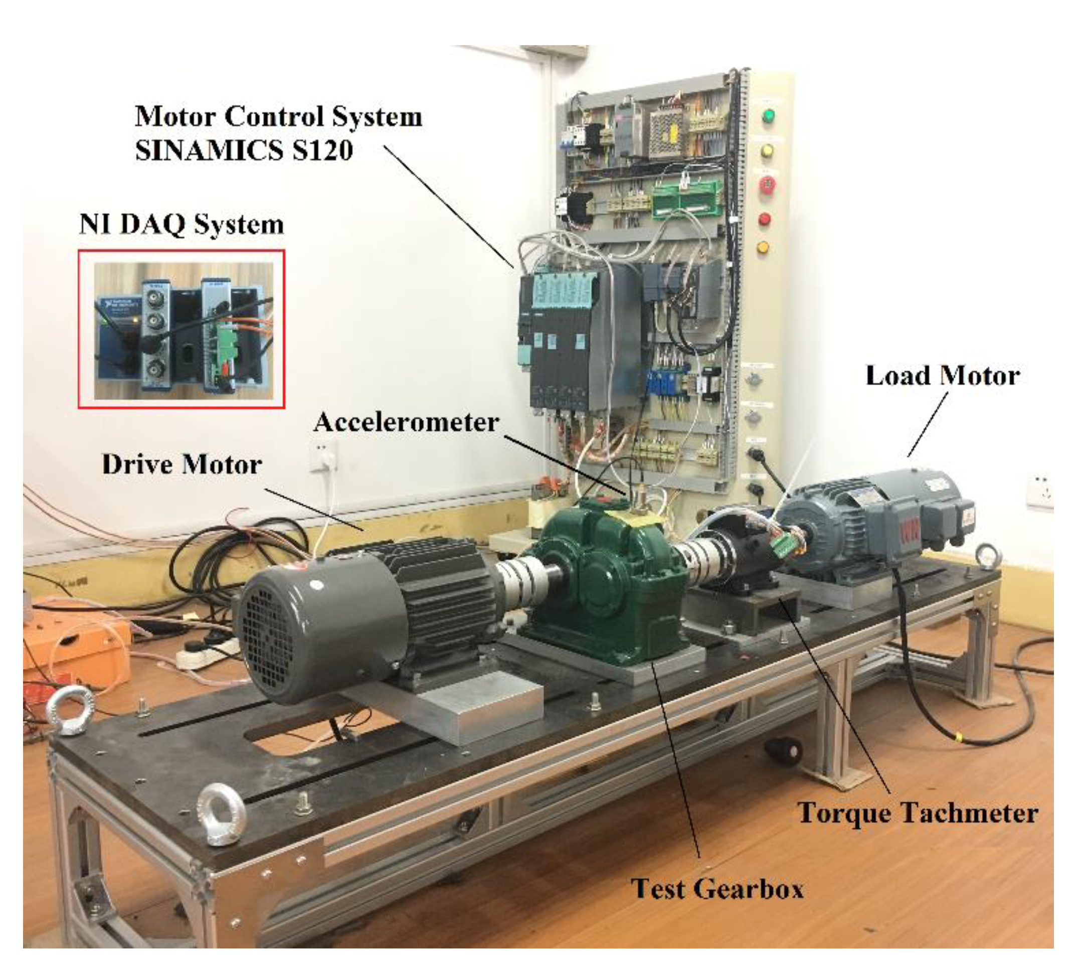
To verify the performance of the proposed method, a scaled-down test-rig was designed and built in a laboratory environment in Figure 3, which was simulated as an integral system of the wind turbine. Two three-phase asynchronous induction motors were fixed on both ends of the bed. One motor was operated as the mechanical power source under the torque-control mode, while the other was simulated under the speed-control mode as the generator. Both motors were driven by a high-performance motion control system. The controlling torque and speed curves were obtained from the kinetics model of the original wind turbine. In this study, the roller bearing fixed in the gearbox was operated under simulated conditions, such as in wind turbines. Moreover, a data acquisition chassis, a National Instruments cDAQ-9132 (2016, National Instruments, Austin, TX, USA), combined with a NI-9401 digital input/output module and an analog NI-9234 voltage input module, was adopted to collect the operational data. An integral piezoelectric accelerometer was adopted to gather the vibration signal by the NI 9234. The rotational speed and torque signal were acquired by the torque-tachometer connected with the NI-9401. The interface software LabVIEW 2017 was programmed to control the motion and collect the data series. The parameters of the piezoelectric accelerometer were 50 g for the range and 96.7 mV/g for the sensitivity. The frequency response range is from 0.5 Hz to 5 kHz and the excitation current is 2 mA. The corresponding sampling frequency was 2 kHz, and the sampling time was 1 s.

An experimental study was performed to evaluate the effectiveness of the proposed method. Four rolling bearings were set with different fault conditions. The defects in the outer races were introduced as small rectangular slits cut using electro-discharge machining. The rectangular slit is 3 mm wide with 0.1 mm deep, 3 mm wide with 0.2 mm deep and 3 mm wide with 0.4 mm deep. The four different bearings, marked as NM, LF, MF and HF, represented the normal-, low-, medium- and high-fault bearings, respectively. The detail for the experimental bearings is shown in

Table 3. Details for the experimental bearings.

No.	Bearing Status	Marked Label	Wearing Defect
1	Normal	NM	None
2	Low fault	LF	0.1 mm × 3 mm
3	Medium fault	MF	0.2 mm × 3 mm
4	High fault	HF	0.4 mm × 3 mm

. In particular, the rotation speed was set at 700 and 1100 rpm. Meanwhile, the torque of the load motor was set at 0.5 and 2 N·m.

4.2. Permutation Entropy Analysis

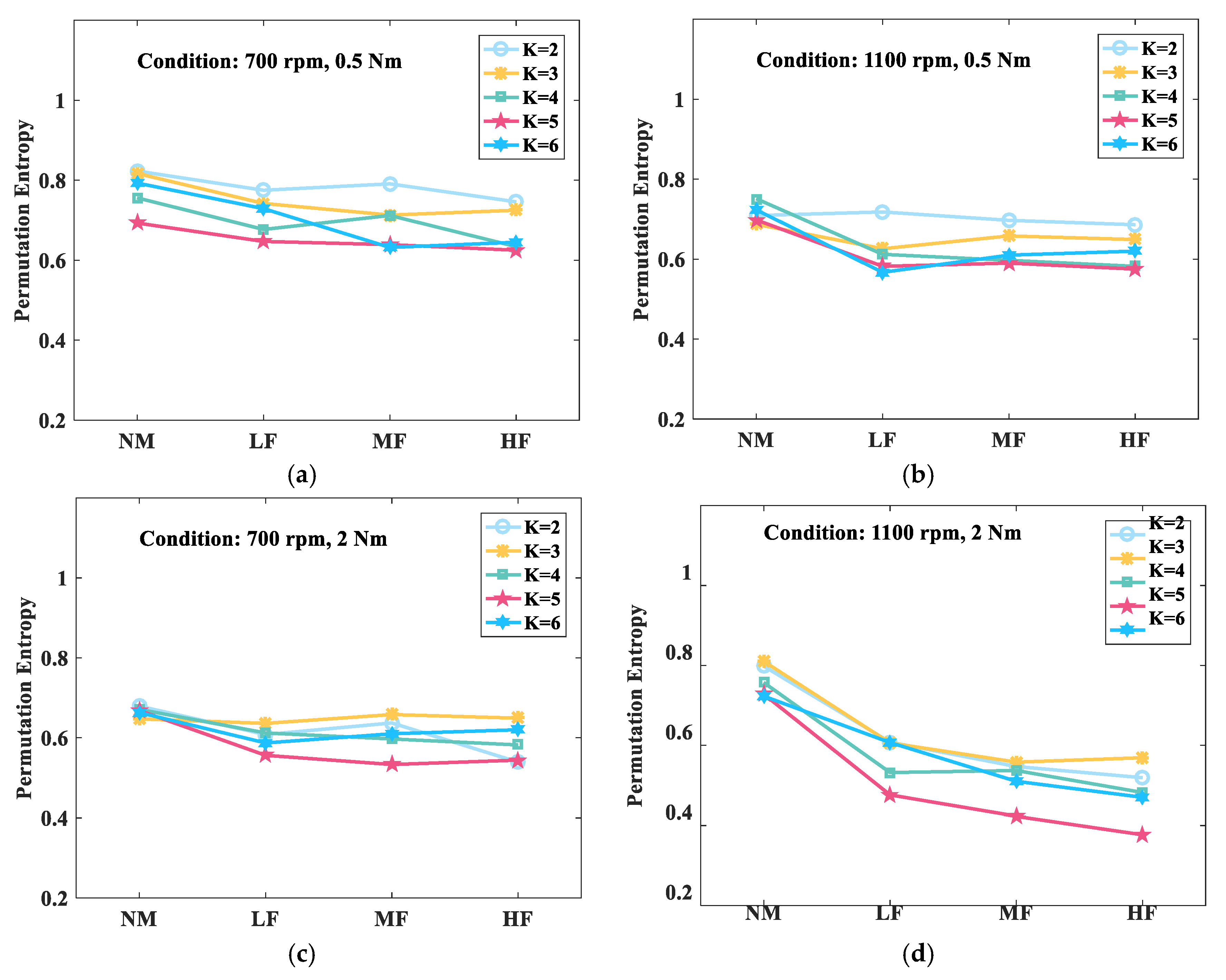
As mentioned above, the permutation energy is selected as one of the statistical input features for the classification. However, the permutation energy varied with the different levels of the VMD method. Hence, the determination of the decomposition level is important for feature extraction. Figure 4 shows the variation result of the permutation entropy with different decomposed levels for the different defective bearings. This figure showed that the fluctuating operating conditions affected the permutation entropy of the worn bearings in the same decomposed levels. To be specific, Figure 4a–d represents permutation entropy results in four different condition of 700 rpm/0.5 N·m, 1100 rpm/0.5 nm, 700 rpm/2 N·m, and 1100 rpm/2 N·m, correspondingly. For instance, when the decomposed level K was 5, the permutation entropy of the low fault bearing was 0.64 in the operating conditions of 700 rpm and 0.5 N·m. Meanwhile, the entropy value dropped to 0.49 in the operating conditions of 1100 rpm and 2 N·m. In addition, by analyzing the overall trend, the permutation entropy value decreased with the wear status of the bearings. For another instance, when the decomposed level K was 5, the permutation entropy of the bearings in different wear conditions decreased from 0.74 to 0.39, under the operating conditions of 1100 rpm and 2 N·m.

Based on the observation, the following can be concluded: (1) for a specific operating condition, the permutation entropy value exhibited a decreasing trend in the wear status of the bearings; (2) for a specific bearing, the permutation entropy value decreased slowly with an increasing rotation speed and load torque; and (3) the selection of the decomposed level K had an influence on the permutation entropy of the defective bearings.

From the experimental result, it was determined that the permutation entropy had the ability to recognize the wear status of the bearings under fluctuating conditions. Nevertheless, it is noticeable that the permutation entropy did not behave monotonically when the decomposed level K was 2, 3 and 6. As a result, the determination of the decomposed level K was vital during the VMD process. The small number of IMFs resulted in a lack of decomposition while the large number of IMFs led to excessive decomposition. Therefore, the analysis of the permutation entropy not only depends on the wear status of the bearings but also relies on the determination of the VMD level K. Particularly, it should be noted that the condition monitoring based on the entropy analysis alone may lead to inaccurate or even incorrect results. Consequently, the multi-feature fusion will be discussed in detail as follows.

4.3. Multifeature Fusion

Considering the weakness of the single-feature analysis, multi-feature fusion is adopted to evaluate the health condition of the bearings. In the extraction process from the fault information, the feature vectors of the sample sets need to be normalized. Since the elements of feature sets have different units, the numerical value must be normalized. In this paper, the min–max normalization method is imported in Equation (13) as follows, where the Z_i is the normalized result, F_max is the maximum data of the vector, F_min is the minimum data, respectively.

$$Z_i=\frac{F_i-F_{\min }}{F_{\max }-F_{\min }}$$

(13)

Then, the feature selection method is applied to filter the redundant features. According to the calculated values of the Fisher score, the highly distinguishable features were sorted from the original vectors, which were then fed into the SVM model for the wearing-status classification. As referred to in Subsection 2.4, the stratified sampling method was employed for the multiclass SVM in this study case, which treated one class at a time as well as other classes combined. By utilizing this method, the negative sample sets were more representative in the training set, guaranteeing that the SVM model is more robust than the traditional random sampling.

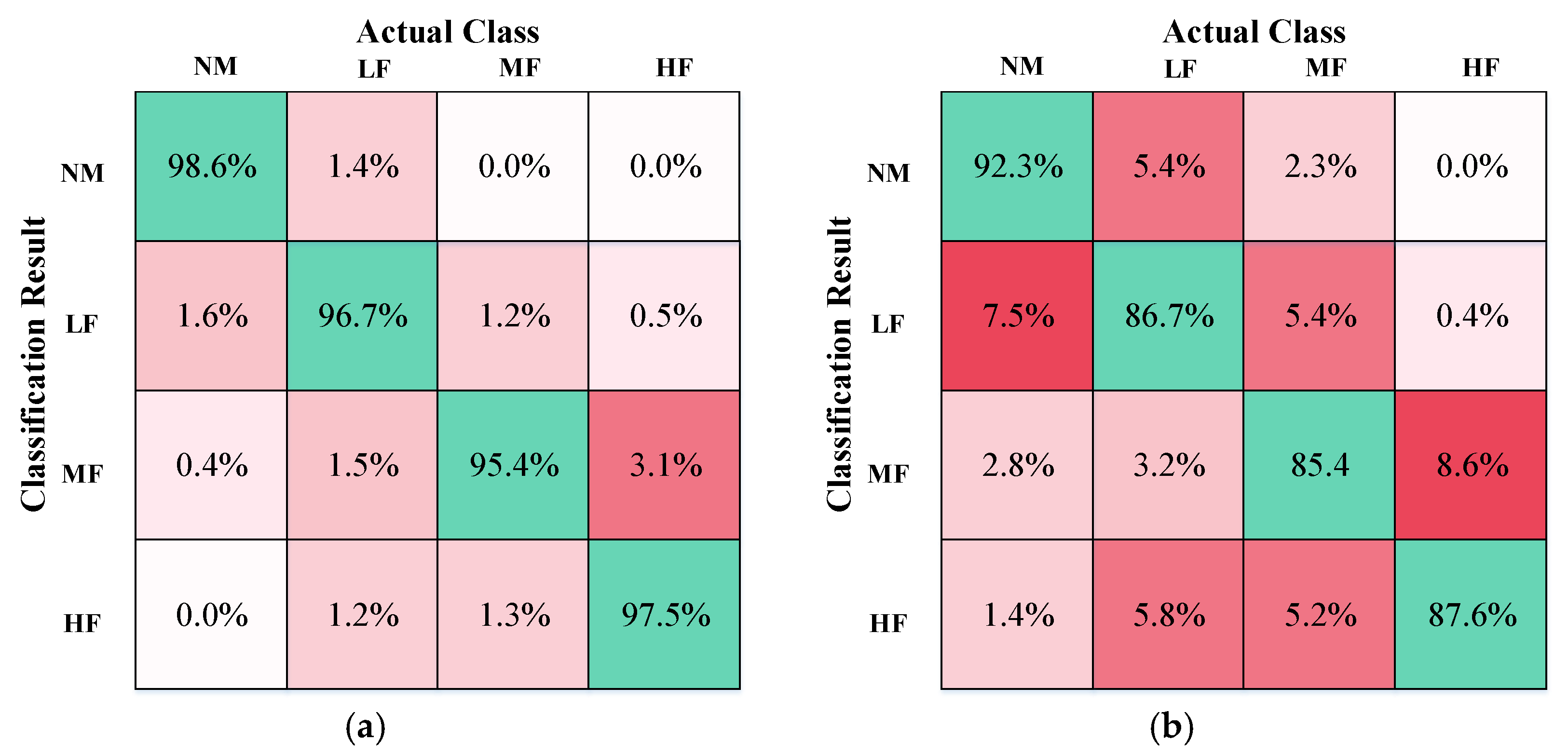
Figure 5a shows the classification results obtained by utilizing the Fisher score method for feature selection. Figure 5b shows the classification results by adopting all 20 features without optimized selection. As observed from the table of results, the classification accuracy was better by distinguishing the relevant features. Certainly, the computational burden would also be relieved, since the dimensions of the feature vector were reduced. For comparison, the ratio of the samples for the training set to the test set is 1:4. Twenty percent of the sample sets were selected for training, and the other 80% of the sample sets were generated for testing. The final statistical results were calculated for 200 trials.

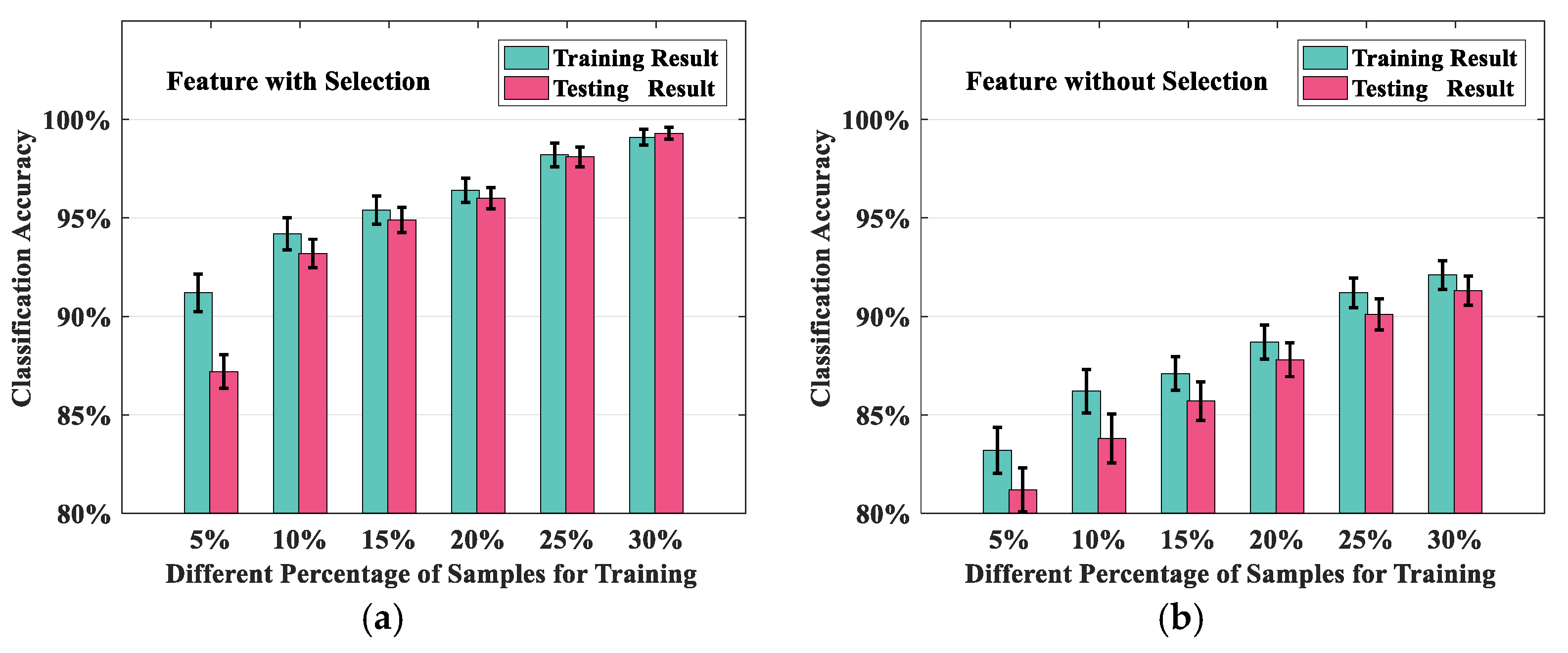
To further investigate the effectiveness of the feature selection, we performed the proposed method by using different ratios of training and testing sets. The percentages for training were increased by 5%, 10%, 15%, 20%, 25% and 30%. To reduce the random effects, 1000 trials were performed for each training set percentage. The samples were obtained and chosen under different operational conditions. Figure 6a,b shows the error bar graphs from averaging the accuracy values for the training and testing results. The error standard deviations are also marked. In particular, the top 10 features were selected for the classification training. The details of the number of features selected are discussed later in the next paragraph. Comparing Figure 6a,b, it was observed that the training and test accuracy values with the feature selection was better than the accuracy values without the feature selection. When the training percentage was selected as 5%, the difference between the training and test accuracy values was larger than 5%, which demonstrated that the SVM training model was underfitting. Obviously, for each subfigure, the testing accuracy was enhanced with the increased percentage of the training sets, while the classification error decreased. When the training percentage increased to 30%, the training and test accuracy values were close to those of the feature selection method. However, without feature selection, the training and test results did not achieve consistency regardless of the training set percentages from 5% to 30%. The comparison results verified the necessity of the feature selection process.

In this case, the SVM and artificial neural network (ANN) classifiers were applied to demonstrate the effect of the number of selected features. The sample sets were partitioned into 10 equal folds, and the tests were performed for 10 iterations. The number of test instances was 1000. The embedded dimension parameter of the permutation entropy was set to 6. The time delay parameter of the permutation entropy was set as 1. For the SVM classifier, the penalty parameter was set to 20, and the radial basis kernel was selected as the kernel function. For the ANN classifier, a topology with 1 hidden layer was constructed. The sensory units of the input layer are fed into the mentioned features including the statistical information in time domain, energy and entropy. In particular, the number of the sensory units is equal with the selected feature. Four neurons are set in the output layer because of the binary coding. Moreover, in our experiment, the best number of neurons is 16. The learning rate was set to 0.3, and the momentum was set to 0.2 for the multilayer perceptron. Two feature-ranking methods, the Fisher score and ReliefF algorithm, were used for the feature selection. 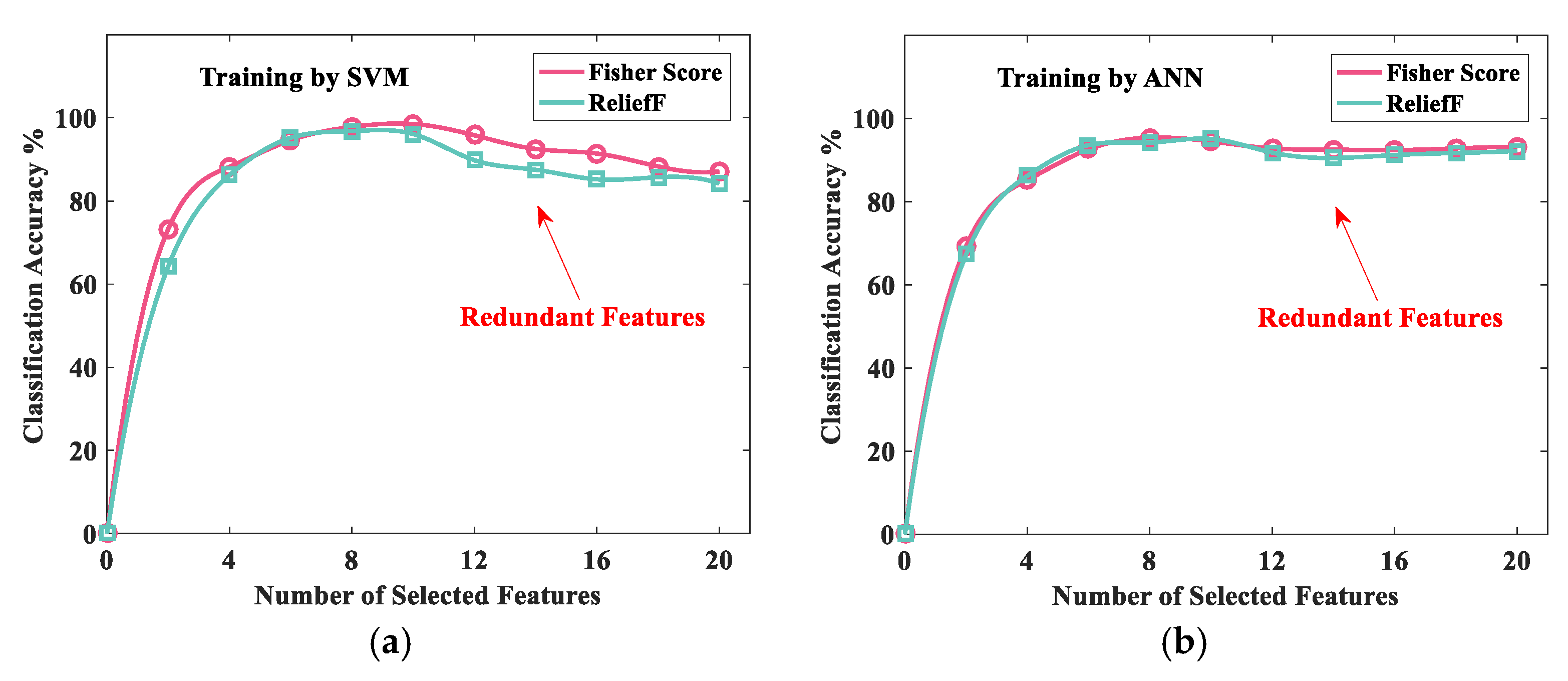Figure 7 shows the accuracy results by extracting different features through these two methods, where Figure 7a,b presents training results by SVM model and ANN model, correspondingly. It was observed that the prediction accuracy of the SVM classifier achieved 98.6% when the top 10 ranked features were selected by the Fisher score method. Similarly, the accuracy of the SVM classifier with the ReliefF algorithm reached 97.6% when the classifiers were fed the 10 top-ranked features. The ANN classifier also gave a similar prediction accuracy with the 8 top-ranked features. However, the SVM classifier with the Fisher scoring method showed better performance in identifying defective bearings, particularly in varying operational conditions.

Interestingly, from the accuracy trend obtained, it was noted that the diagnostic accuracy was enhanced at first with the increased number of ranked features. However, once the dimensionality of the feature vectors was larger than the optimized selected number, the identification performance decreased.

4.4. Performance Analysis

In this article, the performance of the proposed method was depicted with the following values: precision for the correctly identified defective bearings, P_defect; recall for the correctly identified defective bearings, R_defect; precision for the incorrectly identified defective bearings, P_other; and recall for the incorrectly identified defective bearings, R_other.

$$\begin{array}{l}{P}_{defect}=\frac{TP}{TP+FP}\\ R_{defect}=\frac{TP}{TP+FN}\\ P_{other}=\frac{TN}{TN+FN}\\ R_{other}=\frac{FP}{FP+TN}\end{array}$$

(14)

TP represents the number of true positive instances, which means that the defected bearing is identified correctly. FP represents the number of false positive instances, which means that another bearing is identified as the monitored defective bearing incorrectly. FN represents the number of false negative instances, which means that the defected bearing is incorrectly identified as another bearing. TN represents the number of true negative instances, which means that another bearing was correctly identified as the monitored defective bearing. The SVM classifier with the Fisher score method was trained with the training dataset The classification threshold was set to 0.5. The cost values C and γ of the SVM model were set to 100 and 0.02, respectively. Considering the robustness of the identification of the defective bearings under fluctuating conditions, four datasets were selected to evaluate the performance of the proposed method. Each dataset was obtained in different operational conditions, which are presented in

Table 4. The performance of the proposed method for different datasets.

	Pdefect	Rdefect	Pother	Rother
Dataset I 700 rpm, 0.5 N·m	96.7%	93.7%	92.4%	98.6%
Dataset II 1100r pm, 0.5 N·m	97.5%	94.6%	97.2%	96.8%
Dataset III 700 rpm, 2 N·m	96.4%	94.3%	95.7%	98.5%
Dataset IV 1100 rpm, 2 N·m	95.2%	92.9%	94.5%	98.9%

in detail.

The performance of the proposed method on different datasets is summarized in Table 4. The average results of P_defect, R_defect, P_other and R_other were 96.7%, 93.7%, 92.4% and 98.6% for Dataset I, respectively, under conditions of 700 rpm and 0.5 N·m. For Dataset II, the values were 97.5%, 94.6%, 97.2% and 96.8%, respectively, under conditions of 1100 rpm and 0.5 N·m. For Dataset III, under conditions of 1100 rpm and 0.5 N·m, the results were 96.4%, 94.3%, 95.7% and 98.5%, respectively, and for Dataset IV, the results were 95.2%, 92.9%, 94.5% and 98.9%. From Table 4, the statistical results show that the proposed method causes low false positives. However, the false negative cases were relatively higher than the false positive cases. This result reflects the fact that the proposed classifier was able to identify the fault level of the defect bearing accurately, avoiding the increase in the false alarm rate.

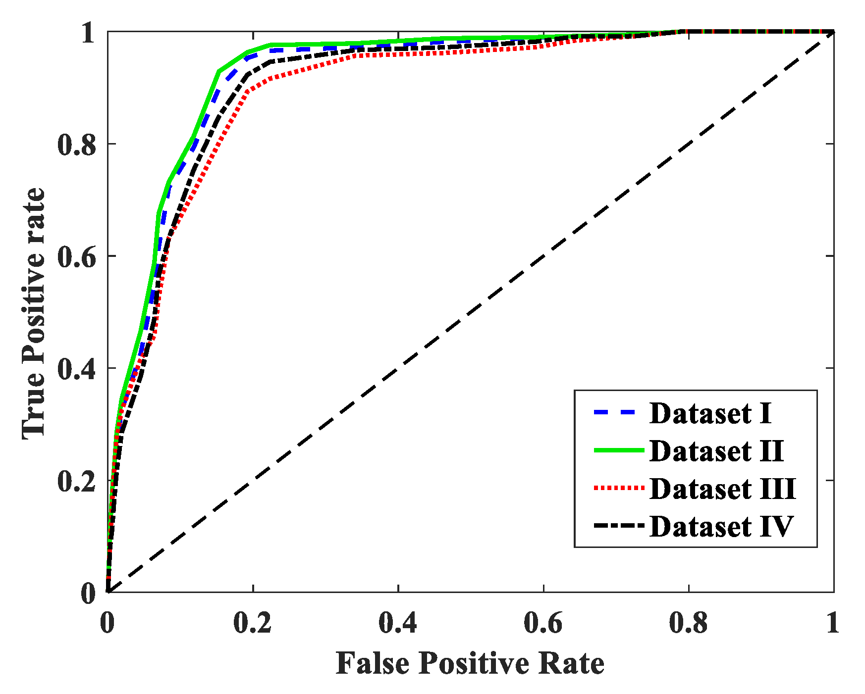
As an evaluation method for the classifier, the receiver operating characteristic (ROC) value has been widely used to depict the tradeoff relationship between the true positive rate and the false positive rate. Figure 8 shows the four ROC curves to represent the true positive rate versus the false positive rate, which were calculated by a varying the threshold value θ. The threshold value was varied from 0 to 1 with a step of 0.02. The areas of the four ROC curves were 0.923, 0.931, 0.901 and 0.912, as shown in Figure 9. To be specific, Figure 9a showed the ROC value in SVM training model, which is aimed to analyze the classifier performance with different selected features. Meanwhile Figure 9b shows the ROC value by ANN training model, correspondingly. For the condition monitoring prediction, a large false positive rate would incur a higher cost, due to the unnecessary maintenance for the wind turbine, than would a small true positive rate. Inversely, a small true positive rate would also degrade the usefulness of the condition monitoring system. Observed from the ROC curves, the proposed method has sufficient flexibility to satisfy various requirements, either for the fault-detection sensitivity or specificity.

In addition, as mentioned in Section 3.1, the selected feature threshold value is very important. In Figure 7, it can be observed that the top 10 ranked features are proper in Fisher score. Meanwhile the ROC values verify that the top 12 ranked features are proper in Fisher score for SVM model as well as the ANN model. Combined with the selection results in Figure 1, we choose the Fisher score threshold as 0.3, and the ReliefF threshold as 0.2.

5. Conclusions

This paper presents a new evaluation method for rolling bearings in a fluctuating operational environment. By utilizing the variational mode decomposition, the vibration signal was decomposed to obtain a set of intrinsic mode functions. The statistical approach and the permutation entropy were adopted to extract the corresponding features, which helped to improve the feature extraction capability. Subsequently, feature selection methods, the Fisher score and ReliefF algorithm, were introduced to rank the relevant features based on the scores from high to low. The reconstructed feature vectors were fed into the SVM classifier for training to identify the health condition of the bearings. Several experiments were performed and analyzed to investigate the validity of the proposed method. The conclusions of this research are summarized as follows. The permutation entropy analysis had the ability to recognize the wear status of the bearings under fluctuating conditions. Nevertheless, the determination of the decomposed level K was vital during the VMD process. In particular, it should be noted that condition monitoring based on an entropy analysis alone may lead to inaccurate or even incorrect results. Moreover, the feature selection process is beneficial and vital for the health evaluation of the bearings. By distinguishing the relevant and irrelevant features, both the accuracy of the identification results and the computational efficiency will be improved. In particular, the Fisher score method showed better performance in ranking the relevant features under varying operational conditions. The proposed method can mitigate the adverse impact of fluctuating the wind turbine conditions and permit the identification of the real bearing state more effectively. From the performance analysis, the proposed method showed sufficient flexibility to satisfy various requirements, either for fault-detection sensitivity or specificity.

In future studies, the selection of the VMD parameters will be optimized using information entropy theory rather than in an experiential determination. Additionally, the semisupervised on-line learning method will be utilized to handle the unlabeled data at the training stage in the proposed work.

References

1. Bishop, I.D.; Miller, D.R. Visual assessment of off-shore wind turbines: The influence of distance, contrast, movement and social variables. Renew. Energy 2007, 32, 814–831. [Google Scholar] [CrossRef]
2. Gibbons, S. Gone with the Wind: Valuing the visual impacts of wind turbines through house prices. J. Environ. Econ. Manag. 2015, 72, 177–196. [Google Scholar] [CrossRef]
3. Yu, T.H.; Behm, H.; Bill, R.; Kang, J.A. Audio-visual perception of new wind parks. Landsc. Urban Plan. 2017, 165, 1–10. [Google Scholar] [CrossRef]
4. Michaud, D.S.; Feder, K.; Keith, S.E.; Voicescu, S.A.; Marro, L.; Than, J.; Guay, M.; Denning, A.; McGuire, D.; Bower, T.; et al. Exposure to wind turbine noise: Perceptual responses and reported health effects. J. Acoust. Soc. Am. 2016, 139, 1443–1454. [Google Scholar] [CrossRef] [PubMed] [Green Version]
5. Gallo, P.; Fredianelli, L.; Palazzuoli, D.; Licitra, G.; Fidecaro, F. A procedure for the assessment of wind turbine noise. Appl. Acoust. 2016, 114, 213–217. [Google Scholar] [CrossRef]
6. Fredianelli, L.; Carpita, S.; Licitra, G. A procedure for deriving wind turbine noise limits by taking into account annoyance. Sci. Total Environ. 2019, 648, 728–736. [Google Scholar] [CrossRef]
7. Fredianelli, L.; Licitra, G.; Gallo, P.; Palazzuoli, D. The suitable parameters to assess noise impact of a wind farm in a complex terrain: A case-study in Tuscan hills. In Proceedings of the EURONOISE 2012, Prague, Czech Republic, 10–13 June 2012. [Google Scholar]
8. Qian, P.; Ma, X.; Zhang, D.; Wang, J. Data-driven condition monitoring approaches to improving power output of wind turbines. IEEE Trans. Ind. Electron. 2019, 66, 6012–6020. [Google Scholar] [CrossRef]
9. Stetco, A.; Dinmohammadi, F.; Zhao, X.; Robu, V.; Flynn, D.; Barnes, M.; Keane, J.; Nenadic, G. Machine learning methods for wind turbine condition monitoring: A review. Renew. Energy 2019, 133, 620–635. [Google Scholar] [CrossRef]
10. Tan, C.K.; Irving, P.; Mba, D. A comparative experimental study on the diagnostic and prognostic capabilities of acoustics emission, vibration and spectrometric oil analysis for spur gears. Mech. Syst. Signal Process. 2007, 21, 208–233. [Google Scholar] [CrossRef] [Green Version]
11. Sharma, V.; Parey, A. Gear crack detection using modified TSA and proposed fault indicators for fluctuating speed conditions. Measurement 2016, 90, 560–575. [Google Scholar] [CrossRef]
12. He, M.; He, D.; Yoon, J.; Nostrand, T.J.; Zhu, J.; Bechhoefer, E. Wind turbine planetary gearbox feature extraction and fault diagnosis using a deep-learning-based approach. Proc. Inst. Mech. Eng. Part O J. Risk Reliab. 2019, 233, 303–316. [Google Scholar] [CrossRef]
13. Inturi, V.; Sabareesh, G.R.; Supradeepan, K.; Penumakala, P.K. Integrated condition monitoring scheme for bearing fault diagnosis of a wind turbine gearbox. J. Vib. Control 2019, 25, 1852–1865. [Google Scholar] [CrossRef]
14. Shen, Y.; Zhu, Z.; Wang, S.; Wang, G. Dynamic analysis of tapered thin-walled beams using spectral finite element method. Shock Vib. 2019, 2019, 2174209. [Google Scholar] [CrossRef]
15. Zhang, M.; Wang, T.; Tang, T.; Benbouzid, M.; Diallo, D. An imbalance fault detection method based on data normalization and EMD for marine current turbines. ISA Trans. 2017, 68, 302–312. [Google Scholar] [CrossRef] [PubMed]
16. Yang, D.; Li, H.; Hu, Y.; Zhao, J.; Xiao, H.; Lan, Y. Vibration condition monitoring system for wind turbine bearings based on noise suppression with multi-point data fusion. Renew. Energy 2016, 92, 104–116. [Google Scholar] [CrossRef]
17. Wang, D.; Tse, P.W.; Tsui, K.L. An enhanced kurtogram method for fault diagnosis of rolling element bearings. Mech. Syst. Signal Process. 2013, 35, 176–199. [Google Scholar] [CrossRef]
18. Lei, Y.; Lin, J.; He, Z.; Zi, Y. Application of an improved kurtogram method for fault diagnosis of rolling element bearings. Mech. Syst. Signal Process. 2011, 25, 1738–1749. [Google Scholar] [CrossRef]
19. Dragomiretskiy, K.; Zosso, D. Variational mode decomposition. IEEE Trans. Signal Process. 2014, 62, 531–544. [Google Scholar] [CrossRef]
20. Li, Z.; Jiang, Y.; Guo, Q.; Hu, C.; Peng, Z. Multi-dimensional variational mode decomposition for bearing-crack detection in wind turbines with large driving-speed variations. Renew. Energy 2018, 116, 55–73. [Google Scholar] [CrossRef]
21. Igba, J.; Alemzadeh, K.; Durugbo, C.; Eiriksson, E.T. Analysing RMS and peak values of vibration signals for condition monitoring of wind turbine gearboxes. Renew. Energy 2016, 91, 90–106. [Google Scholar] [CrossRef] [Green Version]
22. Yang, W.; Court, R.; Jiang, J. Wind turbine condition monitoring by the approach of SCADA data analysis. Renew. Energy 2013, 53, 365–376. [Google Scholar] [CrossRef]
23. Dempsey, P.J.; Sheng, S. Investigation of data fusion applied to health monitoring of wind turbine drivetrain components. Wind Energy 2013, 16, 479–489. [Google Scholar] [CrossRef]
24. Feng, Y.; Qiu, Y.; Crabtree, C.J.; Long, H.; Tavner, P.J. Monitoring wind turbine gearboxes. Wind Energy 2013, 16, 728–740. [Google Scholar] [CrossRef]
25. Yang, W.; Tavner, P.J.; Crabtree, C.J.; Feng, Y.; Qiu, Y. Wind turbine condition monitoring: Technical and commercial challenges. Wind Energy 2012, 17, 673–693. [Google Scholar] [CrossRef]
26. Kusiak, A.; Verma, A. Monitoring wind farms with performance curves. IEEE Trans. Sustain. Energy 2013, 4, 192–199. [Google Scholar] [CrossRef]
27. Schlechtingen, M.; Santos, I.F.; Achiche, S. Wind turbine condition monitoring based on SCADA data using normal behavior models. Part 1: System description. Appl. Soft Comput. 2013, 13, 259–270. [Google Scholar] [CrossRef]
28. Wang, T.; Han, Q.; Chu, F.; Feng, Z. Vibration based condition monitoring and fault diagnosis of wind turbine planetary gearbox: A review. Mech. Syst. Signal Process. 2019, 126, 662–685. [Google Scholar] [CrossRef]
29. Marri, K.; Swaminathan, R. Classification of muscle fatigue in dynamic contraction using surface electromyography signals and multifractal singularity spectral analysis. J. Dyn. Syst. Meas. Control 2016, 138, 111008. [Google Scholar] [CrossRef]
30. Li, Y.; Feng, K.; Liang, X.; Zuo, M.J. A fault diagnosis method for planetary gearboxes under non-stationary working conditions using improved Vold-Kalman filter and multi-scale sample entropy. J. Sound Vib. 2019, 439, 271–286. [Google Scholar] [CrossRef]
31. Zhang, X.; Zhang, Q.; Chen, M.; Sun, Y.; Qin, X.; Li, H. A two-stage feature selection and intelligent fault diagnosis method for rotating machinery using hybrid filter and wrapper method. Neurocomputing 2018, 275, 2426–2439. [Google Scholar] [CrossRef]
32. Hestenes, M.R. Multiplier and gradient methods. J. Optim. Theory Appl. 1969, 4, 303–320. [Google Scholar] [CrossRef]
33. Wang, Y.; Liu, F.; Jiang, Z.; He, S.; Mo, Q. Complex variational mode decomposition for signal processing applications. Mech. Syst. Signal Process. 2017, 86, 75–85. [Google Scholar] [CrossRef]
34. Munoz-Guillermo, M. Ordinal Patterns in Heartbeat Time Series: An Approach Using Multiscale Analysis. Entropy 2019, 21, 583. [Google Scholar] [CrossRef]
35. Boskoski, P.; Gasperin, M.; Petelin, D.; Juricic, D. Bearing fault prognostics using Renyi entropy based features and Gaussian process models. Mech. Syst. Signal Process. 2015, 52, 327–337. [Google Scholar] [CrossRef]
36. Zhu, T.; Qu, Z.; Xu, H.; Zhang, J.; Shao, Z.; Chen, Y.; Prabhakar, S.; Yang, J. RiskCog: Unobtrusive real-time user authentication on mobile devices in the wild. IEEE Trans. Mob. Comput. 2019. [Google Scholar] [CrossRef]
37. Ding, S.F.; Zhao, X.Y.; Zhang, J.; Zhang, X.K.; Xue, Y. A review on multi-class TWSVM. Artif. Intell. Rev. 2019, 52, 775–801. [Google Scholar] [CrossRef]
Figure 1. The correlation between the feature and classification accuracy according to the Fisher score and ReliefF algorithm. (a) correlation results in Fisher score; (b) correlation results in ReliefF.
Energies 12 03085 g001
Figure 2. Main framework of the proposed method.
Energies 12 03085 g002
Figure 3. Setup of the experimental test-rig.
Energies 12 03085 g003
Figure 4. The permutation entropy with varying decomposed levels under different conditions. (a) Condition in 700 rpm/0.5 N·m; (b) condition in 1100 rpm/0.5 N·m; (c) condition in 700 rpm/2 N·m; (d) condition in 1100 rpm/2 N·m.
Energies 12 03085 g004
Figure 5. The comparison results for the feature selection using the support vector machine (SVM) classification (20% training data). (a) confusion matrix with feature selection in Fisher score; (b) confusion matrix without feature selection.
Energies 12 03085 g005
Figure 6. Comparison of the accuracy of the SVM and artificial neural network (ANN) classifiers with different training percentage. (a) classification accuracy with feature selection in Fisher score; (b) classification accuracy without feature selection.
Energies 12 03085 g006
Figure 7. Identification accuracy results with different numbers of selected features. (a) train result by SVM model; (b) train result by ANN model.
Energies 12 03085 g007
Figure 8. Receiver operating characteristic (ROC) curve for the four different datasets.
Energies 12 03085 g008
Figure 9. Receiver operating characteristic value by using the SVM and ANN. (a) ROC value by SVM training model; (b) ROC value by ANN training model.
Energies 12 03085 g009