Wavelet Scale Variance Analysis of Wind Extremes in Mountainous Terrains


Abstract
1. Introduction
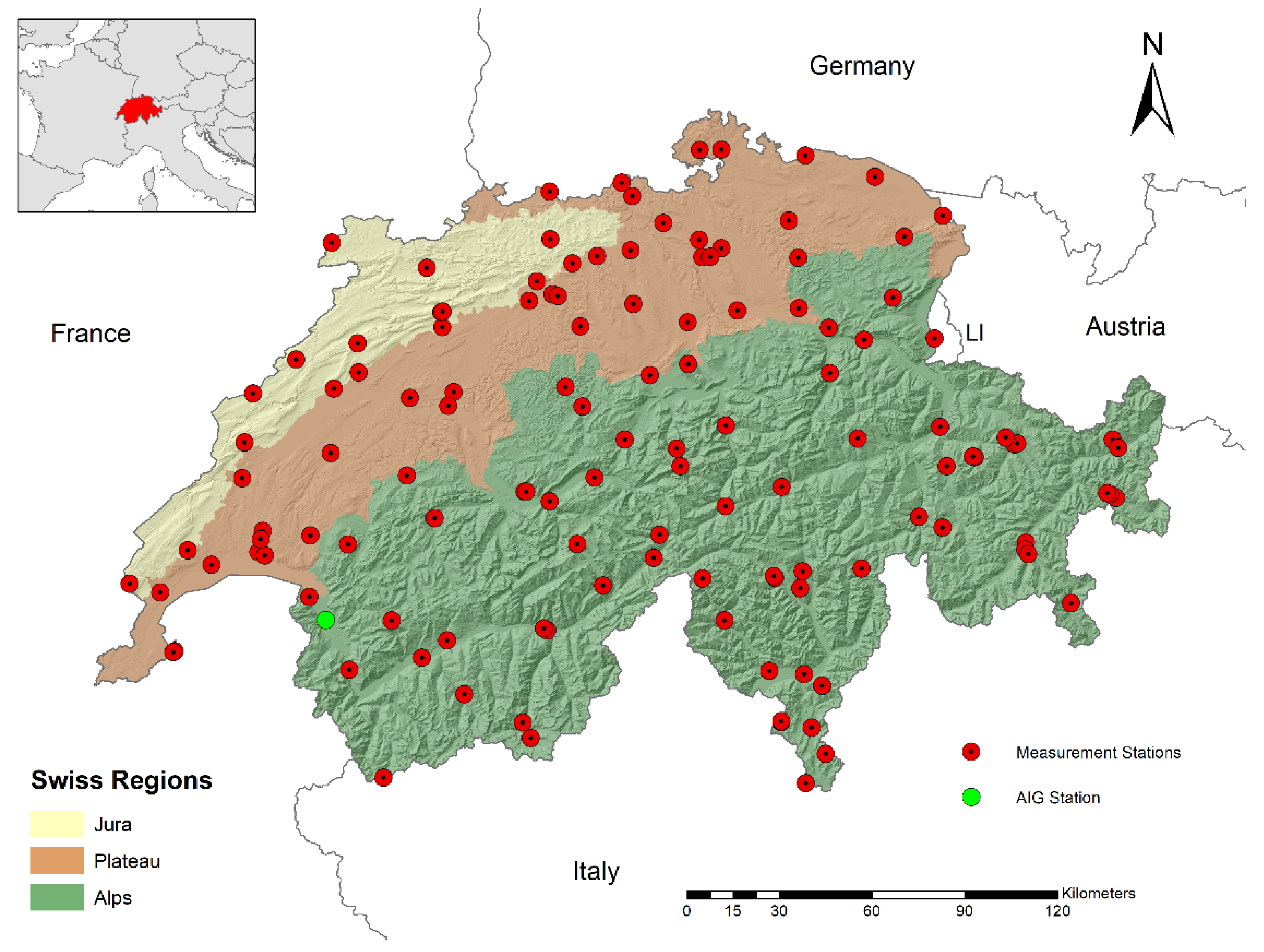
2. Data
3. Methods
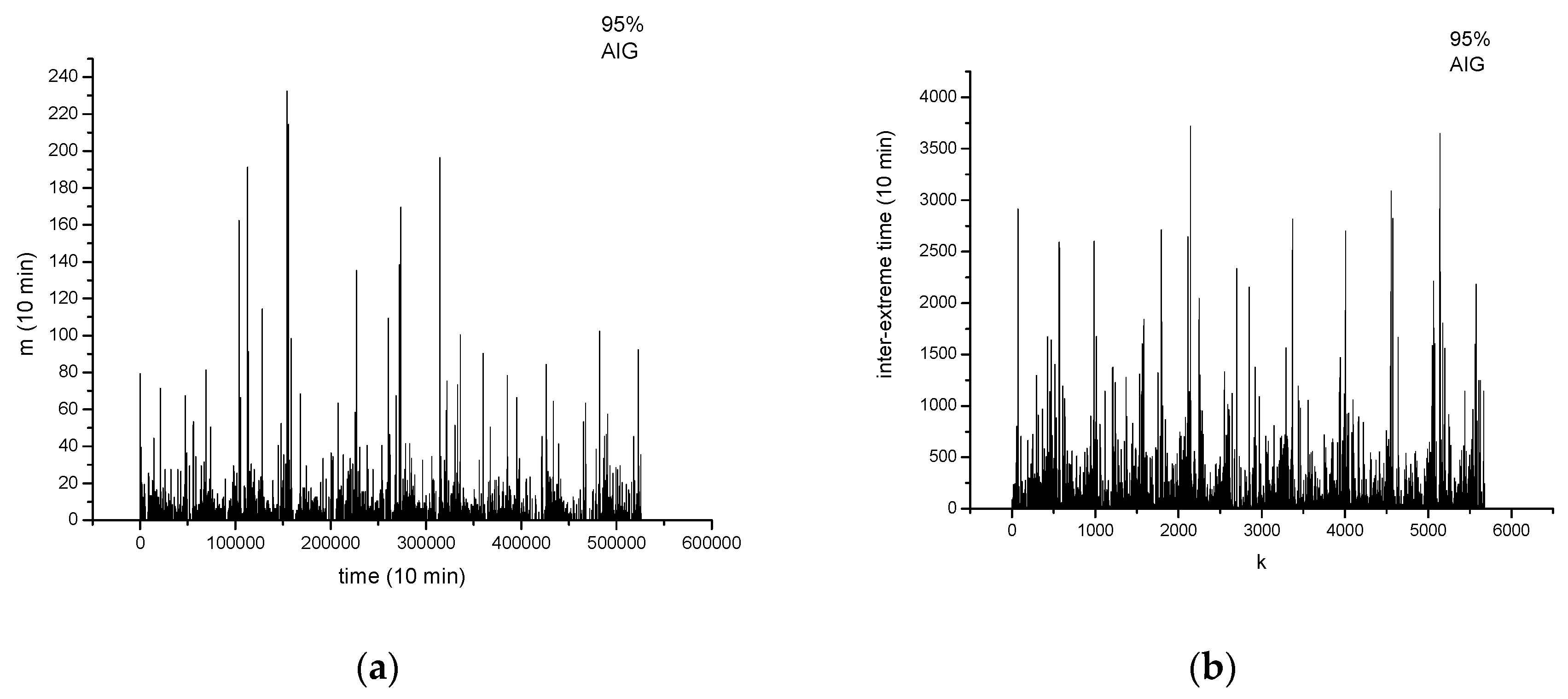
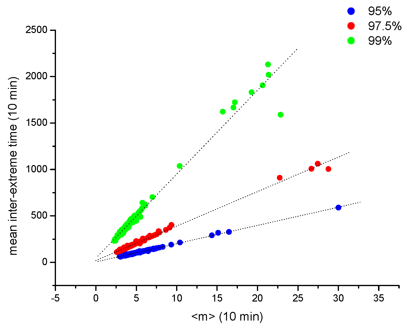
3.1. Definition of Wind Extremes and Their Statistical Features
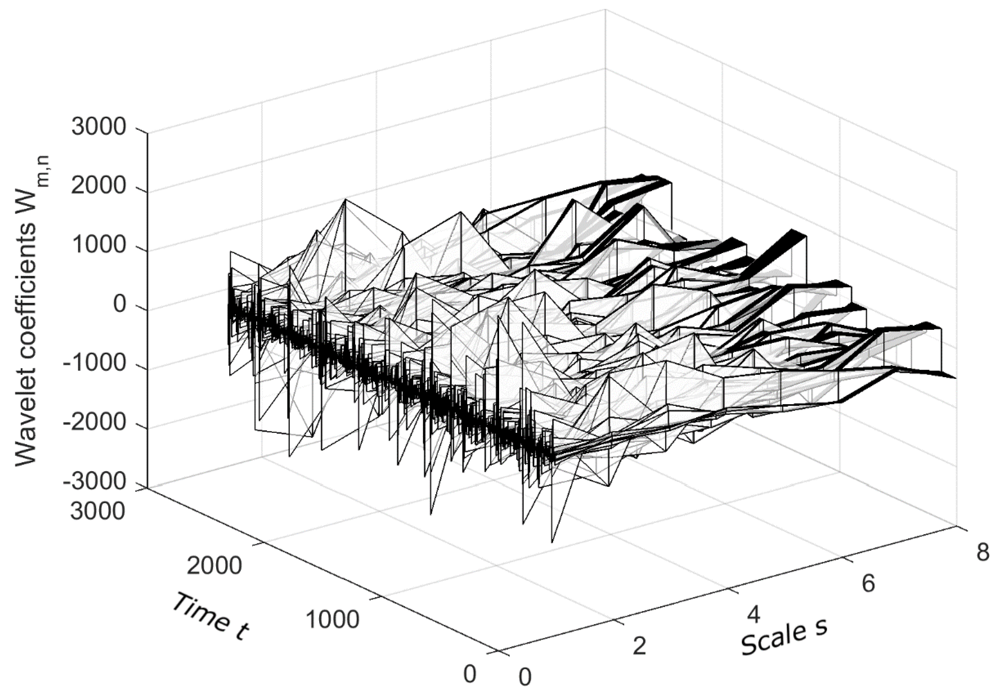
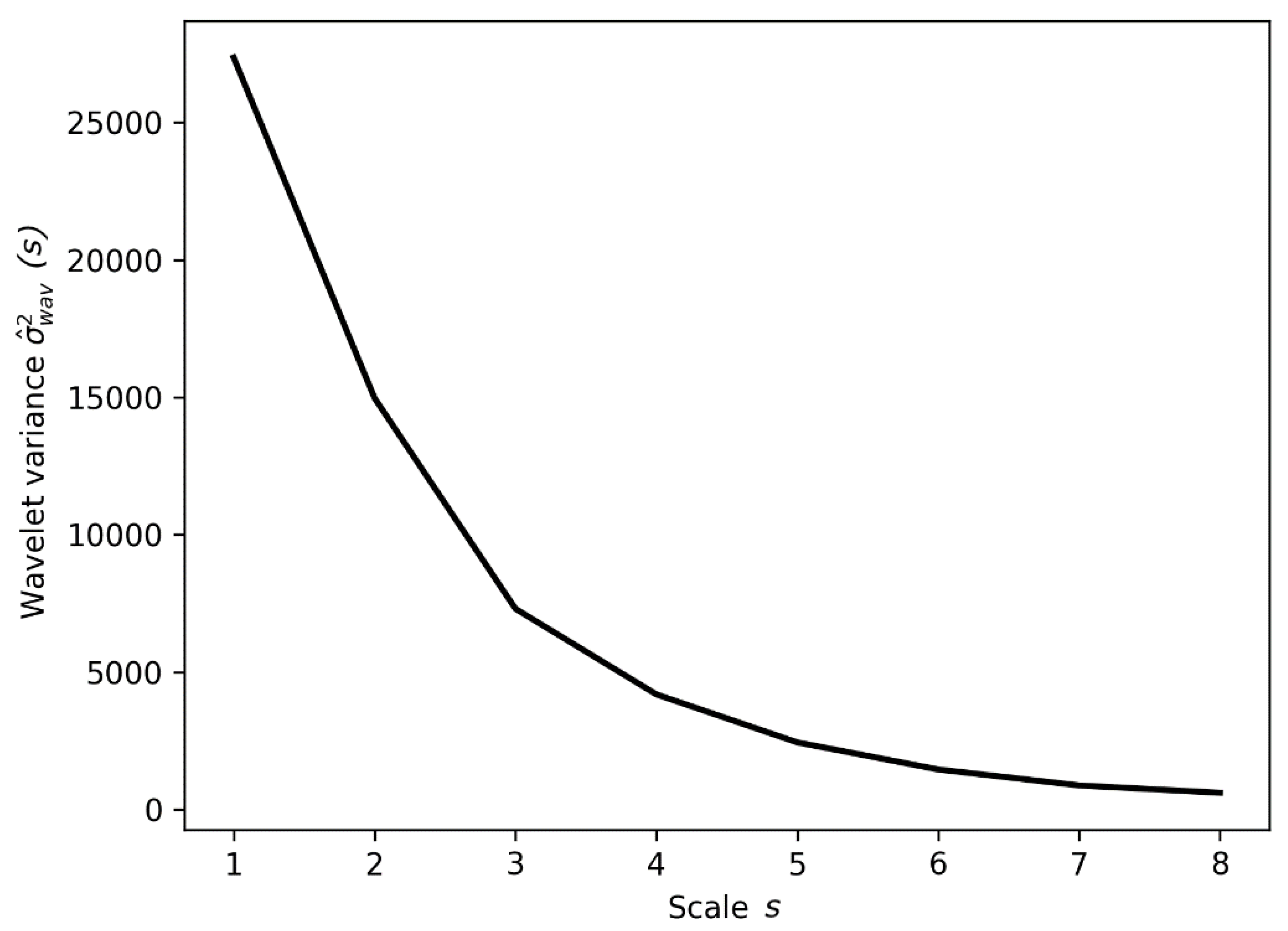
3.2. The Wavelet Variance
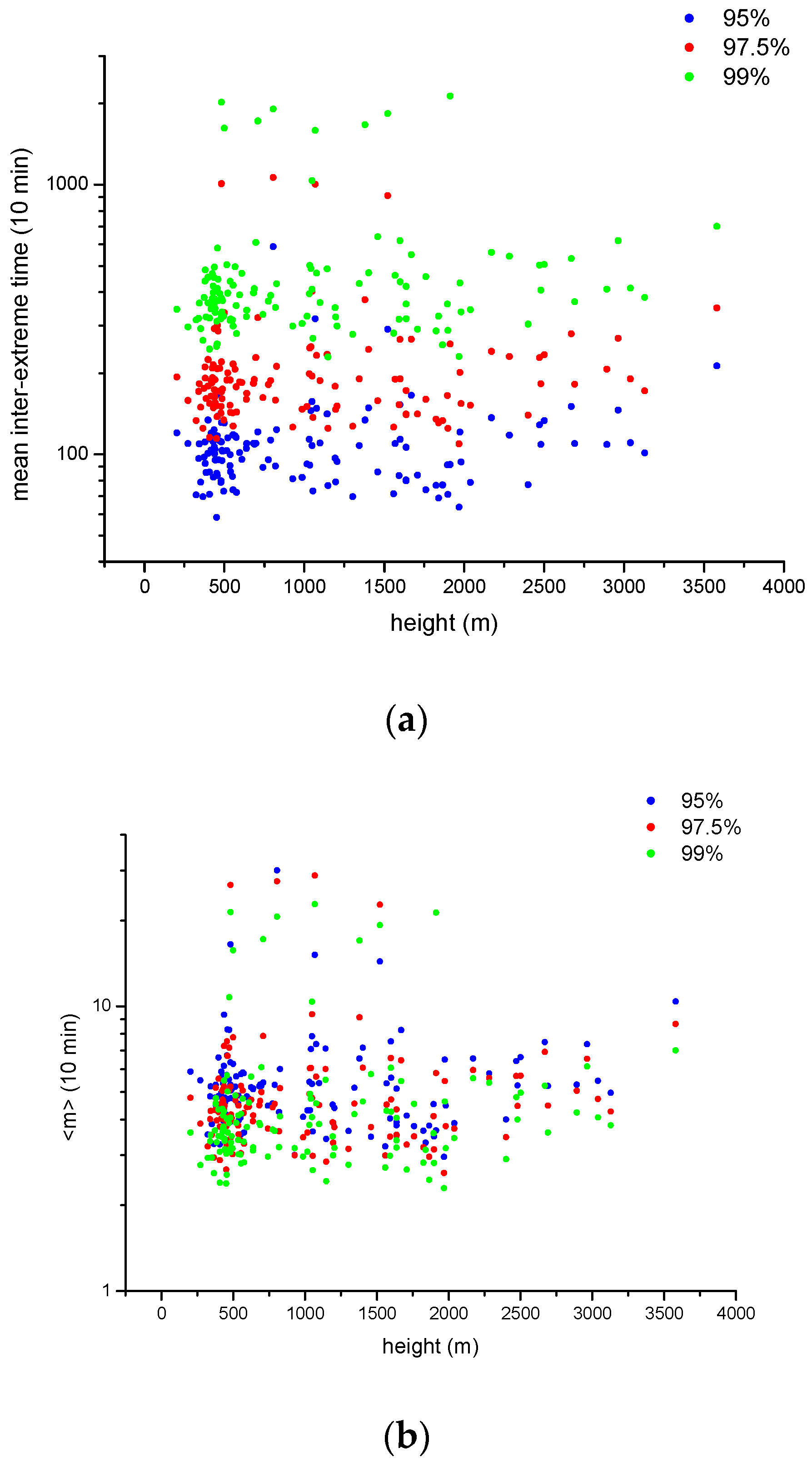
4. Results
5. Conclusions
Author Contributions
Funding
Conflicts of Interest
References
- Ummels, B.C.; Gibescu, M.; Pelgrum, E.; Kling, W.L.; Brand, A.J. Impacts of Wind Power on Thermal Generation Unit Commitment and Dispatch. IEEE Trans. Energy Convers. 2007, 22, 44–51. [Google Scholar] [CrossRef]
- Demirci, E.; Cuhadaroglu, B. Statistical analysis of wind circulation and air pollution in urban Trabzon. Energy Build. 2000, 31, 49–53. [Google Scholar] [CrossRef]
- Cermak, J.E. Wind-tunnel development and trends in applications to civil engineering. J. Wind Eng. Ind. Aerodyn. 2003, 91, 355–370. [Google Scholar] [CrossRef]
- Sterk, G.; Jacobs, A.F.G.; Van Boxel, J.H. The effect of turbulent flow structures on saltation sand transport in the atmospheric boundary layer. Earth Surf. Proc. Land. 1998, 23, 877–887. [Google Scholar] [CrossRef]
- Kavasseri, R.G.; Nagarajan, R. Evidence of crossover phenomena in wind-speed data. IEEE Trans Circuits Syst. I 2004, 51, 2255–2262. [Google Scholar] [CrossRef]
- Raupach, M.R.; Thom, A.S.; Edwards, I. A wind-tunnel study of turbulent flow close to regularly arrayed rough surfaces. Bound. Layer Meteorol. 1980, 18, 373–397. [Google Scholar] [CrossRef]
- Parsons, D.R.; Walker, I.J.; Wiggs, G.F.S. Numerical modelling of flow structures over idealized transverse aeolian dunes of varying geometry. Geomorphology 2004, 59, 149–164. [Google Scholar] [CrossRef]
- Celik, A.N. A statistical analysis of wind power density based on the Weibull and Rayleigh models at the southern region of Turkey, April 2004. Renew. Energy 2004, 29, 593–604. [Google Scholar] [CrossRef]
- Karakasidis, T.E.; Charakopoulos, A. Detection of low-dimensional chaos in wind time series. Chaos Solit. Fractals 2009, 41, 1723–1732. [Google Scholar] [CrossRef]
- Avdakovic, S.; Lukac, A.; Nuhanovic, A.; Music, M. Wind Speed Data Analysis using Wavelet Transform. Int. J. Environ. Chem. Ecol. Geol. Geophys. Eng. 2011, 5, 138–142. [Google Scholar]
- Kavasseri, R.G.; Nagarajan, R. A multifractal description of wind speed records. Chaos Solit. Fractals 2005, 24, 165–173. [Google Scholar] [CrossRef]
- Kavasseri, R.G.; Nagarajan, R. A qualitative description of boundary layer wind speed records. Fluct. Noise Lett. 2006, 6, 201–213. [Google Scholar] [CrossRef]
- Koçak, K. Examination of persistence properties of wind speed records using detrended fluctuation analysis. Energy 2009, 34, 1980–1985. [Google Scholar] [CrossRef]
- Santos, M.D.O.; Stosic, T.; Stosic, B.D. Long-term correlations in hourly wind speed records in Pernambuco. Braz. Phys. A 2012, 391, 1546–1552. [Google Scholar] [CrossRef]
- Feng, T.; Fu, Z.T.; Deng, X.; Mao, J.Y. A brief description to different multi-fractal behaviors of daily wind speed records over China. Phys. Lett. A 2009, 373, 4134–4141. [Google Scholar] [CrossRef]
- Telesca, L.; Lovallo, M. Analysis of the time dynamics in wind records by means of multifractal detrended fluctuation analysis and the Fisher—Shannon information plane. J. Stat. Mech. 2011, 2001, P07001. [Google Scholar] [CrossRef]
- Telesca, L.; Lovallo, M.; Kanevski, M. Power spectrum and multifractal detrended fluctuation analysis of high-frequency wind measurements in mountainous regions. Appl. Energy 2016, 162, 1052–1061. [Google Scholar] [CrossRef]
- Fu, Z.T.; Li, Q.L.; Yuan, N.M.; Yao, Z.H. Multi-scale entropy analysis of vertical wind variation series in atmospheric boundary-layer. Commun. Nonlinear Sci. Numer. Simul. 2014, 19, 83–91. [Google Scholar] [CrossRef]
- Zeng, M.; Zhang, X.-N.; Li, J.-H.; Meng, Q.-H. The Scaling Properties of High-frequency Wind Speed Records Based on Multiscale Multifractal Analysis. Acta Phys. Pol. B 2016, 47, 2205–2224. [Google Scholar] [CrossRef]
- Walker, I.J. Physical and logistical considerations of using ultrasonic anemometers in aeolian sediment transport research. Geomorphology 2005, 68, 57–76. [Google Scholar] [CrossRef]
- Martius, O.; Pfahl, S.; Chevalier, C. A global quantification of compound precipitation and wind extremes. Geophys. Res. Lett. 2016, 43, 7709–7717. [Google Scholar] [CrossRef]
- Froidevaux, P.; Schwanbeck, J.; Weingartner, R.; Chevalier, C.; Martius, O. Flood triggering in Switzerland: The role of daily to monthly preceding precipitation. Hydrol. Earth Syst. Sci. 2015, 19, 3903–3924. [Google Scholar] [CrossRef]
- Klawa, M.; Ulbrich, U. A model for the estimation of storm losses and the identification of severe winter storms in Germany. Nat. Hazards Earth Syst. Sci. 2003, 3, 725–732. [Google Scholar] [CrossRef]
- MeteoSwiss. Automatic Monitoring Network, Internal Report. 2018. Available online: https://www.meteoswiss.admin.ch (accessed on 5 August 2019).
- Jun, M.; Stein, M.L. An approach to producing space: Time covariance functions on spheres. Technometrics 2007, 49, 468–479. [Google Scholar] [CrossRef]
- Porcu, E.; Bevilacqua, M.; Genton, M.G. Spatio-temporal covariance and cross-covariance functions of the great circle distance on a sphere. J. Am. Stat. Assoc. 2016, 111, 888–898. [Google Scholar] [CrossRef]
- Cramer, H.; Leadbetter, M.R. Stationary and Related Stochastic Processes; Dover Publications Inc.: Mineaola, NY, USA, 1967. [Google Scholar]
- Lindsay, R.W.; Percival, D.B.; Rothrock, D.A. The discrete wavelet transform and the scale analysis of the surface properties of sea ice. IEEE Trans. Geosci. Rem. Sens. 1996, 34, 771–787. [Google Scholar] [CrossRef]
- Thurner, S.; Feurstein, M.; Teich, M.C. Multiresolution wavelet analysis of heartbeat intervals discriminates healthy patients from those with cardiac pathology. Phys. Rev. Lett. 1997, 80, 1544–1547. [Google Scholar] [CrossRef]
- Daubechies, I. Ten Lectures on Wavelets; Society for Industrial and Applied Mathematics: Philadelphia, PA, USA, 1992. [Google Scholar]
- Addison, P.S. The Illustrated Wavelet Transform Handbook; Taylor & Francis: Didcot/Abingdon, UK, 2002. [Google Scholar]
- Helbig, N.; Mott, R.; van Herwijnen, A.; Winstral, A.; Jonas, T. Parameterizing surface wind speed over complex topography. J. Geophys. Res. Atmos. 2017, 122, 651–667. [Google Scholar] [CrossRef]
- Jimenez, P.A.; Dudhia, J. Improving the representation of resolved and unresolved topographic effects on surface wind in the WRF model. J. Appl. Meteorol. Climatol. 2012, 51, 300–316. [Google Scholar] [CrossRef]


| 95% Threshold | 97.5% Threshold | 99% Threshold | |||||
|---|---|---|---|---|---|---|---|
| Scale | r | p-Value | r | p-Value | r | p-Value | |
| Δx = 25 m | 1 | 0.19 | 0.039 | 0.19 | 0.033 | 0.27 | 0.002 |
| 2 | 0.19 | 0.032 | 0.21 | 0.019 | 0.24 | 0.007 | |
| 3 | 0.17 | 0.059 | 0.19 | 0.034 | 0.26 | 0.003 | |
| 4 | 0.17 | 0.067 | 0.17 | 0.061 | 0.21 | 0.018 | |
| 5 | 0.15 | 0.109 | 0.21 | 0.016 | 0.17 | 0.059 | |
| 6 | 0.22 | 0.015 | 0.24 | 0.006 | −0.13 | 0.138 | |
| 7 | 0.23 | 0.011 | −0.13 | 0.147 | - | - | |
| 8 | 0.00 | 0.999 | - | - | - | - | |
| 95% Threshold | 97.5% Threshold | 99% Threshold | |||||
|---|---|---|---|---|---|---|---|
| Scale | r | p-Value | r | p-Value | r | p-Value | |
| Δx = 25 m | 1 | 0.19 | 0.034 | 0.20 | 0.026 | 0.25 | 0.004 |
| 2 | 0.21 | 0.018 | 0.22 | 0.011 | 0.24 | 0.006 | |
| 3 | 0.21 | 0.018 | 0.22 | 0.011 | 0.23 | 0.009 | |
| sbg 250 m | 1 | 0.25 | 0.005 | 0.25 | 0.004 | 0.30 | 0.001 |
| 2 | 0.26 | 0.003 | 0.28 | 0.001 | 0.28 | 0.001 | |
| 3 | 0.25 | 0.004 | 0.26 | 0.003 | 0.28 | 0.001 | |
| sbg 1000 m | 1 | 0.23 | 0.008 | 0.22 | 0.011 | 0.28 | 0.001 |
| 2 | 0.23 | 0.007 | 0.24 | 0.006 | 0.24 | 0.006 | |
| 3 | 0.21 | 0.016 | 0.23 | 0.009 | 0.26 | 0.003 | |
| 95% Threshold | 97.5% Threshold | 99% Threshold | |||||
|---|---|---|---|---|---|---|---|
| Scale | r | p-Value | r | p-Value | r | p-Value | |
| Δx = 25 m | 1 | 0.18 | 0.037 | 0.17 | 0.055 | 0.15 | 0.089 |
| 2 | 0.20 | 0.022 | 0.18 | 0.043 | 0.15 | 0.082 | |
| 3 | 0.22 | 0.012 | 0.20 | 0.023 | 0.11 | 0.206 | |
| Δx = 250 m | 1 | 0.16 | 0.062 | 0.16 | 0.075 | 0.17 | 0.054 |
| 2 | 0.15 | 0.083 | 0.14 | 0.118 | 0.18 | 0.035 | |
| 3 | 0.15 | 0.081 | 0.17 | 0.056 | 0.21 | 0.019 | |
| Δx = 1000 m | 1 | 0.27 | 0.002 | 0.31 | 0.000 | 0.28 | 0.001 |
| 2 | 0.27 | 0.002 | 0.27 | 0.002 | 0.30 | 0.001 | |
| 3 | 0.28 | 0.001 | 0.32 | 0.000 | 0.28 | 0.001 | |
© 2019 by the authors. Licensee MDPI, Basel, Switzerland. This article is an open access article distributed under the terms and conditions of the Creative Commons Attribution (CC BY) license (http://creativecommons.org/licenses/by/4.0/).
Share and Cite
Telesca, L.; Guignard, F.; Helbig, N.; Kanevski, M. Wavelet Scale Variance Analysis of Wind Extremes in Mountainous Terrains. Energies 2019, 12, 3048. https://doi.org/10.3390/en12163048
Telesca L, Guignard F, Helbig N, Kanevski M. Wavelet Scale Variance Analysis of Wind Extremes in Mountainous Terrains. Energies. 2019; 12(16):3048. https://doi.org/10.3390/en12163048
Chicago/Turabian StyleTelesca, Luciano, Fabian Guignard, Nora Helbig, and Mikhail Kanevski. 2019. "Wavelet Scale Variance Analysis of Wind Extremes in Mountainous Terrains" Energies 12, no. 16: 3048. https://doi.org/10.3390/en12163048
APA StyleTelesca, L., Guignard, F., Helbig, N., & Kanevski, M. (2019). Wavelet Scale Variance Analysis of Wind Extremes in Mountainous Terrains. Energies, 12(16), 3048. https://doi.org/10.3390/en12163048