Smart Meter Data-Based Three-Stage Algorithm to Calculate Power and Energy Losses in Low Voltage Distribution Networks †


Abstract
1. Introduction
- Secure transmission of data to the consumers, the DNOs, or another operator (for example Metering Operator);
- Bidirectional communication between the smart meters installed at consumer/producers and the data concentrators (information management points) belonging to the DNO;
- Remote controlled connection/disconnection from the network or demand limitation at the consumers;
- Implementing differentiated time-of-use tariffs.
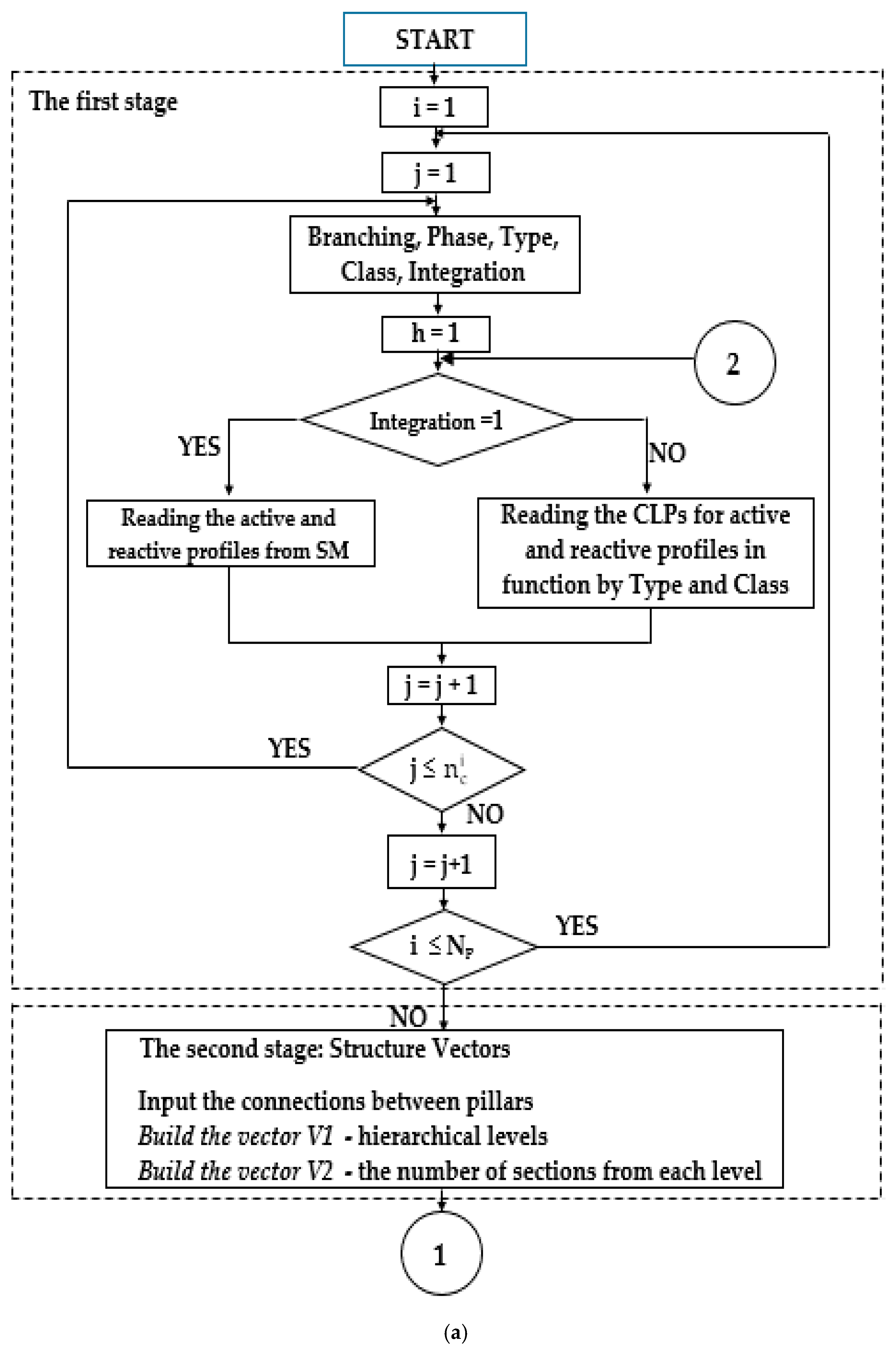
- Stage I is based on the online work, with files from two different databases, as follows: The database of the SMS, including the consumption and production profiles for the integrated consumers and producers and the database containing the characteristic load profiles (CLPs) obtained from the profiling process, which are assigned to the consumers with installed conventional meters, non-integrated in the SMS. This work mode enables the algorithm to work online to estimate the power losses.
- Stage 2 implements a recognition function of the network topology based on two structure vectors.
- Stage 3 is based on an improved version of a forward/backward sweep-based algorithm to quickly calculate fast the power/energy losses in three-phase LV distribution networks with balanced and unbalanced operating regimes. Regarding the forward/backward sweep-based algorithm, it was mainly used in the medium voltage distribution networks to calculate the balanced symmetric steady-state regime [25,26,27,28]. However, the proposed version was adapted to the LV distribution networks that most often operate in unbalanced regimes due to the chaotic allocation of the single-phase consumers on the phases.
2. Three-Stage Algorithm to Calculate Power/Energy Losses
- Stage 1. The input data of the consumers, referring to the energy characteristics, are read from the databases of the DNO, which contain the load profiles of each consumer integrated in the SMS or the CLPs, if the consumer has a conventional meter non-integrated in the SMS. Additionally, the production profiles of the producers from the network are loaded by the algorithm.
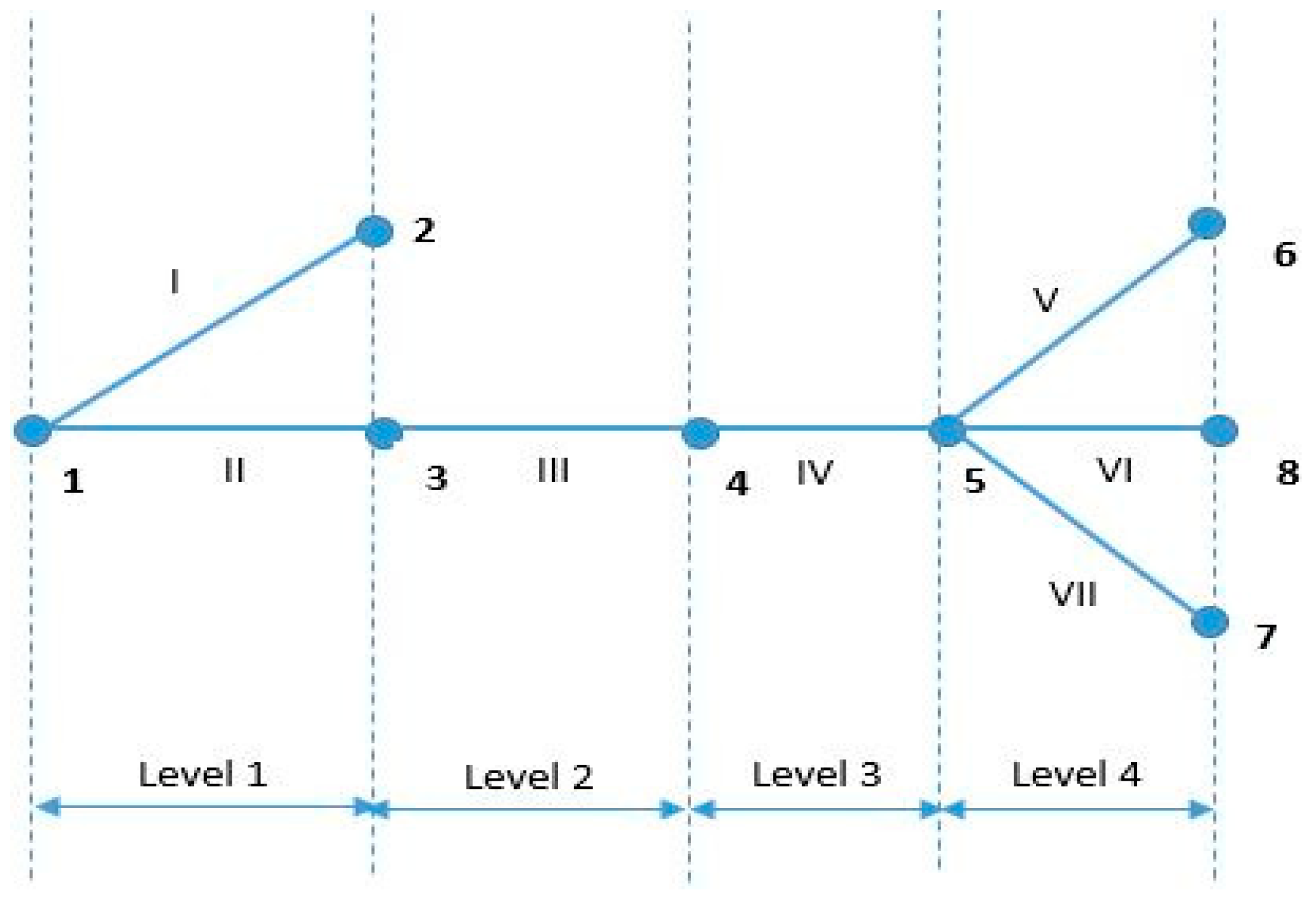
- Stage 2. The architecture of network is established using an efficient algorithm based on two structure vectors.
- Stage 3. The power/energy losses are determined using an improved variant forward/backward sweep algorithm, which can work in the balanced and unbalanced operating regimes, with or without distributed generation.
2.1. The First Stage
- The energy consumption is monitored online with benefits for both parts, the DNOs can implement the energy efficiency measures, and the consumers can establish their pricing mode in function by the energy consumption behaviour.
- The analysis of recorded data must lead to optimal strategies regarding the increase of energy efficiency in the LV distribution networks of the DNOs.
- Extending the processed data (as load type profiles) to the networks from the same area, but without SMS implementation, to analyse their operation regime.
- Number represents the allocated record for a certain consumer in the database of the DNO.
- Pillar represents the identification number of each pillar made by the DNO for a rural LV distribution network. The pillars are numbered in all rural LV distribution networks to know where the consumers are connected. For example, in Table 1 consumer 1 is connected at pillar 1 and consumer 4 is connected at pillar 3.
- Branching identifies the type of electric branching for each consumer, single-phase or three-phases. These can be identified in the database with 1-P (single-phase) or 3-P (three-phases).
- Phase allows for identification of the phase(s) at which a consumer is allocated (the notations a, b, or c can be seen for a 1-P consumer, and the notation abc can be observed for a 3-P consumer).
- Type emphasizes if the consumer belongs in the following consumption patterns: Residential (ID is 1); non-residential, namely community buildings, hospitals, town halls, schools, etc. (ID is 2); commercial (ID is 3); and industrial (ID is 4).
- Class belongs to a certain Type, identified by the annual electric energy consumption of the consumer. The DNO can classify the consumers in a given number of consumer classes in function of different criteria. As an example, a division into five classes (made by a DNO from Romania) for the consumers from residential/non-residential types [28] is the following: Class_1 (0–400 kWh), Class_2 (400–1250 kWh), Class_3 (1250–2500 kWh), Class_4 (2500–3500 kWh), and Class_5 (>3500 kWh).
- Integration allows the user to know if the meter is (value is equal to 1) or is not (value is equal to 0) in the database of the SMS. If the meter is integrated, based on the ID of the meter, the active and reactive power profiles of the consumer can be loaded from the database. If a meter is not integrated, then the daily energy indexes will be loaded from the database. In this last case, a CLP will be allocated to the consumer using the approach presented in the next section in function of the records Type and Class. The associated active and reactive power profile is finally obtained based on the loaded energy indexes.
Load Profiling Process Based on Smart Meters Data
2.2. The Second Stage
2.3. The Third Stage
- Step 3.1. The currents at the level of the nodes (pillars) are calculated:where k is the index of current iteration and Kmax expresses the maximum value of iterations initially introduced by the decision maker.
- Step 3.2. The current flow on each section (v–i) of the network are calculated:where v is the pillar in up stream of pillar i, Next (i) is the set of pillars next to the pillar i, and (v–i) is the section.
- Step 4.1. The voltage drop on the phases {p} of all sections is calculated:where Zv,i and Zv,i0 are the impedances of the phase {p} = {a, b, c} and neutral conductors (0). The value Iv,i0 represents the current flows on the neutral conductor.
- Step 4.2. The voltage on the phase, {p} = {a, b, c}, for each pillar, i, is calculated:
- Step 4.3. The total apparent power injected to the network is calculated:
- Step 4.4. Testing the stopping condition of iterative process:where εS represents the imposed error by the decision maker to stop the iterative process.
3. Case Study
4. Conclusions
Author Contributions
Funding
Conflicts of Interest
Nomenclature:
| 0 | neutral conductor |
| 1-P | single-phase consumer |
| 3-P | three-phase consumer |
| a, b, c | phases of network |
| abc | three-phase consumer in the input data files |
| CLP | Characteristic Load Profile |
| DNO | Distribution Network Operator |
| DSPF | DigSilent Power Factory |
| j | The index for bus |
| Iv,i{p} | The current flow on each section (v–i), [A] |
| i | The index for pillar |
| k | The index for current iteration |
| Kmax | The maximum number of iterations |
| h | The current hour (h = 1,…, H) |
| H | Total number of hours from the analysed period (H = 24) |
| LV | Low Voltage |
| l | The consumer non-integrated in the SMS (l = 1,…, Nc) |
| MAPE | Mean Average Percentage Error, [%] |
| MPE | Mean Percentage Errors, [%] |
| MV | Medium Voltage |
| n | Consumer with smart meter (n = 1, …, NSM) |
| Nc | Total number of consumers non-integrated in the SMS |
| NP | Total number of pillars |
| NSM | Total number of consumers integrated in the SMS |
| v | The pillar in up stream of pillar i |
| {p} | the set of phases {a, b, c} |
| PA | Proposed algorithm |
| Pg, Qg | The active and reactive power of the generator, [kW], [kVAr] |
| Pc, Qc | The active and reactive absorbed power, [kW], [kVAr] |
| Pl | The denormalized load profile at consumer l, [kW/kWh] |
| Pm | Three-phase feeder measured load profile, [kW] |
| Psm | Active power measured with the smart meter, [kW] |
| Pcor | Denormalized load profiles adjusted by measured load profiles, [kW/kWh] |
| s | The LV side of electric substation |
| Ss{p} | The total apparent power injected to the network on the phases {p} = {a, b, c}, [kVA] |
| SMS | Smart Metering System |
| R | Resistance, [Ω] |
| tc | Type of consumer (residential, non-residential, commercial, and industrial) |
| Ui{p} | The phase voltages from each pillar i =1, …, Np, [V], with {p} = {a, b, c} |
| Us{p} | The phase voltages on the LV side of electric substation, [V], {p} = {a, b, c} |
| V1, V2 | Structure vectors |
| Zv,i | The phase impedance of each section (v–i), [Ω] |
| Zv,i0 | The impedance of neutral conductor of each section (v–i), [Ω] |
| X | Reactance, [Ω] |
| Wl | The daily energy consumption for the consumer l = 1,…, Nc, [kWh] |
| ΔP(h) | The deviation between the measured and computed load profiles, [kW], at hour h = 1,…, H |
| ΔUv,i{p} | The voltage drop on the phases {p} = {a, b, c}, on each section (v–i), [V] |
| ΔW | The energy losses, [kWh] |
| εS | The error for the convergence test (Absolute error), [kVA] |
| ε | The absolute error, [kWh] |
| δ | The percentage error, [%] |
Appendix A

| Pillar | Branching | Phase | Consumers Type | Pillar | Branching | Phase | Consumers Type | ||||||||||
|---|---|---|---|---|---|---|---|---|---|---|---|---|---|---|---|---|---|
| 1-P | 3-P | a | b | c | 1 | 2 | 3 | 1-P | 3-P | a | b | c | 1 | 2 | 3 | ||
| 1 | 1 | - | - | 1 | - | 1 | - | - | 96 | 1 | 1 | 1 | 2 | 1 | 1 | - | - |
| 2 | 2 | - | - | 2 | - | 1 | - | - | 97 | 1 | - | - | 1 | - | 1 | - | - |
| 3 | 4 | - | - | 4 | - | 1 | - | - | 98 | 1 | - | - | 1 | - | 1 | - | - |
| 4 | 3 | - | 1 | 2 | - | 1 | - | - | 99 | 6 | - | - | 4 | 2 | 1 | - | - |
| 7 | 3 | - | - | 3 | - | 1 | - | - | 100 | 4 | - | - | 3 | 1 | 1 | - | - |
| 8 | 2 | - | - | 2 | - | 1 | - | - | 101 | 1 | - | - | 1 | - | 1 | - | - |
| 9 | 2 | - | - | 2 | - | 1 | - | - | 102 | 3 | - | - | 3 | - | 1 | - | - |
| 10 | 3 | - | 2 | 1 | - | 1 | - | - | 103 | 1 | - | - | 1 | - | 1 | - | - |
| 11 | 1 | - | - | 1 | - | 1 | - | - | 104 | 1 | - | - | 1 | - | 1 | - | - |
| 12 | 2 | - | - | 2 | - | 1 | - | - | 106 | 2 | - | 1 | - | 1 | 1 | - | - |
| 13 | 1 | - | - | 1 | - | 1 | - | - | 107 | 3 | - | 1 | - | 2 | 1 | - | - |
| 14 | 2 | - | - | - | 2 | 1 | - | - | 109 | 1 | - | - | - | 1 | 1 | - | - |
| 15 | 2 | - | - | 1 | 1 | 1 | - | - | 110 | 1 | - | - | - | 1 | 1 | - | - |
| 17 | - | 1 | 1 | 1 | 1 | 1 | - | - | 111 | 3 | - | - | - | 3 | 1 | - | - |
| 18 | 2 | - | - | - | 2 | 1 | - | - | 112 | 4 | - | - | - | 4 | 1 | - | - |
| 19 | 2 | - | 2 | - | - | 1 | - | - | 113 | 1 | - | - | - | 1 | 1 | - | - |
| 20 | 2 | - | 2 | - | - | 1 | - | - | 114 | 3 | - | - | - | 3 | 1 | - | - |
| 21 | 1 | - | 1 | - | - | 1 | - | - | 115 | 1 | - | - | - | 1 | 2 | - | - |
| 22 | 2 | - | 1 | 1 | - | 1 | - | - | 116 | 1 | - | - | - | 1 | 2 | - | - |
| 23 | 2 | - | 2 | - | - | 1 | - | - | 117 | - | 1 | 1 | 1 | 1 | 1 | - | - |
| 24 | 1 | - | - | - | 1 | 1 | - | - | 118 | - | 1 | 1 | 1 | 1 | 2 | - | - |
| 26 | 2 | - | - | - | 2 | 1 | - | - | 119 | 1 | - | 1 | - | - | 1 | - | - |
| 27 | 3 | - | 1 | - | 2 | 1 | - | - | 120 | 1 | - | 1 | - | - | 1 | - | - |
| 28 | 2 | - | - | 1 | 1 | 1 | - | - | 121 | 2 | - | 2 | - | - | 1 | - | - |
| 29 | 4 | - | - | 1 | 3 | 1 | - | - | 122 | 2 | - | 1 | 1 | - | 1 | - | - |
| 30 | 2 | - | - | - | 2 | 1 | - | - | 123 | 4 | 1 | 2 | 3 | 1 | 1 | - | - |
| 31 | 2 | - | - | - | 2 | 1 | - | - | 124 | 3 | - | 2 | 1 | - | 1 | - | - |
| 32 | 1 | - | - | - | 1 | 1 | - | - | 125 | 2 | - | - | 2 | - | 1 | - | - |
| 33 | 4 | - | - | - | 4 | 1 | - | - | 126 | 2 | - | - | 2 | - | 1 | - | - |
| 34 | 5 | - | - | - | 5 | 1 | - | - | 127 | 2 | - | 1 | - | 1 | 1 | - | - |
| 35 | 4 | - | 1 | 1 | 2 | 1 | - | - | 128 | 2 | - | 2 | - | - | 1 | - | - |
| 36 | 1 | - | - | 1 | - | 1 | - | - | 129 | 4 | - | 4 | - | - | 1 | - | - |
| 37 | 3 | - | - | - | 3 | 1 | - | - | 130 | 1 | - | - | 1 | - | 1 | - | - |
| 38 | 1 | - | - | - | 1 | 1 | - | - | 131 | 3 | - | - | 3 | - | 1 | - | - |
| 39 | 4 | - | - | 1 | 3 | 1 | - | - | 133 | 2 | - | 1 | 1 | - | 1 | - | - |
| 40 | 3 | - | - | - | 3 | 1 | - | - | 134 | 1 | - | - | 1 | - | 1 | - | - |
| 41 | 1 | - | - | - | 1 | 1 | - | - | 135 | 3 | - | 3 | - | - | 1 | - | - |
| 42 | 1 | - | - | - | 1 | 1 | - | - | 136 | 3 | - | 3 | - | - | 1 | - | - |
| 43 | 2 | - | - | - | 2 | 1 | - | - | 137 | 3 | - | - | 3 | - | 1 | - | - |
| 44 | 2 | - | - | 1 | 1 | 1 | - | - | 138 | 2 | - | - | 2 | - | 1 | - | - |
| 45 | 4 | - | - | - | 4 | 1 | - | - | 139 | 1 | - | - | 1 | - | 1 | - | - |
| 46 | 2 | - | - | - | 2 | 1 | - | - | 140 | 3 | 1 | 2 | 3 | 1 | 1 | - | - |
| 47 | 3 | - | 1 | 2 | - | 1 | - | - | 141 | 4 | - | 1 | 3 | - | 1 | - | - |
| 48 | 3 | - | 1 | 2 | - | 1 | 2 | - | 142 | 1 | - | 1 | - | - | 1 | - | - |
| 49 | 2 | - | - | 2 | - | 1 | - | - | 143 | 2 | - | 1 | 1 | - | 1 | - | - |
| 50 | 1 | - | - | - | 1 | 1 | - | - | 144 | 2 | - | 1 | 1 | - | 1 | - | - |
| 51 | 1 | - | - | 1 | - | - | 2 | - | 145 | 2 | - | 1 | - | 1 | 1 | - | - |
| 52 | 3 | - | - | 3 | - | 1 | 2 | - | 146 | 2 | - | 1 | 1 | - | 1 | - | - |
| 53 | 1 | - | - | 1 | - | - | 2 | - | 147 | 1 | - | - | 1 | - | 1 | - | - |
| 54 | 6 | - | - | - | 6 | 1 | 2 | - | 148 | 2 | - | - | 1 | 1 | 1 | - | - |
| 55 | 2 | - | 1 | 1 | - | 1 | - | - | 149 | 1 | - | 1 | - | - | 1 | - | - |
| 56 | 2 | - | - | 2 | - | 1 | - | - | 150 | 3 | - | - | 2 | 1 | 1 | - | - |
| 57 | 1 | - | - | 1 | - | 1 | - | - | 151 | 2 | - | 1 | 1 | - | 1 | - | - |
| 58 | 1 | - | 1 | - | - | 1 | - | - | 152 | 3 | - | 1 | 2 | - | 1 | - | - |
| 59 | 2 | - | - | 2 | - | 1 | - | - | 153 | 1 | - | 1 | - | - | 1 | - | - |
| 60 | 2 | - | 1 | 1 | - | 1 | - | - | 154 | 1 | - | 1 | - | - | 1 | - | - |
| 61 | 1 | - | - | 1 | - | 1 | - | - | 155 | 2 | - | 2 | - | - | 1 | - | - |
| 62 | 1 | - | - | - | 1 | 1 | - | - | 156 | 2 | - | - | 1 | 1 | 1 | - | - |
| 63 | 2 | - | 2 | - | - | 1 | - | - | 157 | 2 | - | 1 | 1 | - | 1 | - | - |
| 65 | 1 | - | - | 1 | - | 1 | - | - | 158 | 2 | - | 1 | 1 | - | 1 | - | - |
| 66 | 4 | - | 1 | 3 | - | 1 | - | - | 159 | 1 | - | - | 1 | - | 1 | - | - |
| 67 | 2 | - | - | 2 | - | 1 | - | - | 161 | 1 | - | 1 | - | - | 1 | - | - |
| 68 | 2 | - | - | 2 | - | 1 | - | - | 162 | 2 | - | - | 2 | - | 1 | - | - |
| 69 | 2 | - | 1 | 1 | - | 1 | - | - | 163 | 1 | - | - | - | 1 | 1 | - | - |
| 70 | 1 | - | - | 1 | - | 1 | - | - | 164 | 3 | - | 2 | - | 1 | 1 | - | - |
| 71 | 1 | - | - | 1 | - | 1 | - | - | 165 | 1 | - | 1 | - | - | 1 | - | - |
| 72 | 1 | - | - | 1 | - | 1 | - | - | 166 | 2 | - | 1 | - | 1 | 1 | - | - |
| 75 | 2 | - | - | 2 | - | 1 | - | - | 168 | 2 | - | 2 | - | - | 1 | - | - |
| 76 | 2 | - | - | 2 | - | 1 | - | - | 169 | 3 | - | 2 | - | 1 | 1 | - | - |
| 77 | 2 | - | 1 | 1 | - | 1 | - | - | 170 | 1 | - | 1 | - | - | 1 | - | - |
| 78 | 4 | - | 1 | 3 | - | 1 | - | - | 171 | 2 | - | - | - | 2 | 1 | - | - |
| 79 | 1 | 1 | 1 | 2 | 1 | 1 | - | - | 172 | 2 | - | - | 1 | 1 | 1 | - | - |
| 80 | 2 | - | 2 | - | 1 | - | - | 173 | 2 | 1 | 2 | 1 | 2 | 1 | - | - | |
| 82 | 2 | - | - | 2 | - | 1 | - | - | 174 | 2 | - | 1 | - | 1 | 1 | - | - |
| 83 | 1 | - | 1 | - | - | 1 | - | - | 175 | 2 | - | - | - | 2 | 1 | - | - |
| 84 | 2 | - | - | 2 | - | 1 | - | - | 176 | 2 | - | 1 | - | 1 | 1 | - | - |
| 86 | 1 | - | - | 1 | - | 1 | - | - | 177 | 2 | - | 1 | - | 1 | 1 | - | - |
| 87 | 2 | - | - | 2 | - | 1 | - | - | 179 | 1 | - | - | - | 1 | 1 | - | - |
| 88 | 1 | - | - | 1 | - | 1 | - | - | 180 | 1 | - | 1 | - | - | 1 | - | - |
| 89 | 2 | - | - | 2 | - | 1 | - | - | 181 | 1 | - | - | - | 1 | 1 | - | - |
| 90 | 1 | - | - | 1 | - | 1 | - | - | 183 | 1 | - | - | - | 1 | 1 | - | - |
| 91 | 2 | - | - | 2 | - | 1 | - | - | 184 | 1 | - | - | - | 1 | 1 | - | - |
| 92 | 1 | - | - | 1 | - | 1 | - | - | 185 | 1 | - | - | 1 | - | 1 | - | - |
| 93 | 2 | - | - | 2 | - | 1 | - | - | 187 | 1 | - | 1 | - | - | 1 | - | - |
| 94 | 1 | - | 1 | - | - | 1 | - | - | 188 | 1 | - | 1 | - | - | 1 | - | - |
| 95 | 1 | - | - | 1 | - | 1 | - | - | 189 | 1 | - | - | - | 1 | 1 | - | - |
| Hour | Main Conductors | Branching Conductors | Total | ||||||
|---|---|---|---|---|---|---|---|---|---|
| a | b | c | Neutral | a | b | c | Neutral | ||
| 1 | 0 | 0.002018 | 0 | 0.002518 | 0 | 0.000253 | 0 | 0.000166 | 0.004955 |
| 2 | 0 | 0.00142 | 0 | 0.001774 | 0 | 0.000175 | 0 | 0.000115 | 0.003484 |
| 3 | 0 | 0.001438 | 0 | 0.001797 | 0 | 0.000176 | 0 | 0.000115 | 0.003527 |
| 4 | 0 | 0.001555 | 0 | 0.001947 | 0 | 0.000189 | 0 | 0.000124 | 0.003815 |
| 5 | 0 | 0.0012 | 0 | 0.001499 | 0 | 0.000145 | 0 | 9.53e-05 | 0.00294 |
| 6 | 0 | 0.001208 | 0 | 0.001508 | 0 | 0.000146 | 0 | 9.58e-05 | 0.002958 |
| 7 | 0 | 0.0015 | 0 | 0.001867 | 0 | 0.000183 | 0 | 0.00012 | 0.00367 |
| 8 | 0 | 0.00154 | 0 | 0.001916 | 0 | 0.000189 | 0 | 0.000124 | 0.003768 |
| 9 | 0 | 0.001351 | 0 | 0.001679 | 0 | 0.000174 | 0 | 0.000114 | 0.003317 |
| 10 | 0 | 0.001747 | 0 | 0.002171 | 0 | 0.000225 | 0 | 0.000148 | 0.004291 |
| 11 | 0 | 0.001319 | 0 | 0.00164 | 0 | 0.000167 | 0 | 1.10e-04 | 0.003237 |
| 12 | 0 | 0.001761 | 0 | 0.002189 | 0 | 0.000227 | 0 | 0.000149 | 0.004326 |
| 13 | 0 | 0.001889 | 0 | 0.002347 | 0 | 0.000245 | 0 | 0.000161 | 0.004641 |
| 14 | 0 | 0.001428 | 0 | 0.001771 | 0 | 0.000185 | 0 | 0.000121 | 0.003505 |
| 15 | 0 | 0.001427 | 0 | 0.001773 | 0 | 0.000185 | 0 | 0.000121 | 0.003506 |
| 16 | 0 | 0.001832 | 0 | 0.002273 | 0 | 0.000236 | 0 | 0.000155 | 0.004497 |
| 17 | 0 | 0.00184 | 0 | 0.002271 | 0 | 0.000255 | 0 | 0.000167 | 0.004533 |
| 18 | 0 | 0.001808 | 0 | 0.002231 | 0 | 0.000247 | 0 | 0.000162 | 0.004448 |
| 19 | 0 | 0.002043 | 0 | 0.002524 | 0 | 0.000277 | 0 | 0.000181 | 0.005026 |
| 20 | 0 | 0.00227 | 0 | 0.002808 | 0 | 0.000312 | 0 | 0.000205 | 0.005595 |
| 21 | 0 | 0.003143 | 0 | 0.003882 | 0 | 0.000443 | 0 | 0.00029 | 0.007758 |
| 22 | 0 | 0.004848 | 0 | 0.005993 | 0 | 0.000661 | 0 | 0.000433 | 0.011936 |
| 23 | 0 | 0.004099 | 0 | 0.005075 | 0 | 0.000568 | 0 | 0.000372 | 0.010114 |
| 24 | 0 | 0.002171 | 0 | 0.002703 | 0 | 0.000268 | 0 | 0.000176 | 0.005318 |
| Total | 0 | 0.046854 | 0 | 0.058157 | 0 | 0.006134 | 0 | 0.00402 | 0.115165 |
| Hour | Main Conductors | Branching Conductors | Total | ||||||
|---|---|---|---|---|---|---|---|---|---|
| a | b | c | Neutral | a | b | c | Neutral | ||
| 1 | 0.0201 | 0.4897 | 0.1064 | 0.3975 | 0.0019 | 0.0103 | 0.0008 | 0.0085 | 1.0350 |
| 2 | 0.0145 | 0.3723 | 0.0782 | 0.3027 | 0.0014 | 0.0084 | 0.0006 | 0.0068 | 0.7848 |
| 3 | 0.0139 | 0.3780 | 0.0837 | 0.3103 | 0.0011 | 0.0086 | 0.0006 | 0.0068 | 0.8030 |
| 4 | 0.0149 | 0.4240 | 0.0879 | 0.3472 | 0.0013 | 0.0102 | 0.0006 | 0.0079 | 0.8940 |
| 5 | 0.0122 | 0.3414 | 0.0728 | 0.2799 | 0.0010 | 0.0083 | 0.0005 | 0.0064 | 0.7226 |
| 6 | 0.0129 | 0.3174 | 0.0776 | 0.2614 | 0.0011 | 0.0067 | 0.0006 | 0.0055 | 0.6833 |
| 7 | 0.0190 | 0.3678 | 0.0983 | 0.3005 | 0.0019 | 0.0065 | 0.0007 | 0.0060 | 0.8008 |
| 8 | 0.0213 | 0.3475 | 0.0993 | 0.2827 | 0.0025 | 0.0053 | 0.0008 | 0.0056 | 0.7648 |
| 9 | 0.0172 | 0.2792 | 0.0716 | 0.2236 | 0.0021 | 0.0042 | 0.0006 | 0.0045 | 0.6030 |
| 10 | 0.0206 | 0.3828 | 0.0930 | 0.3076 | 0.0022 | 0.0065 | 0.0007 | 0.0062 | 0.8197 |
| 11 | 0.0164 | 0.3121 | 0.0734 | 0.2506 | 0.0019 | 0.0056 | 0.0006 | 0.0053 | 0.6659 |
| 12 | 0.0194 | 0.4158 | 0.0902 | 0.3339 | 0.0020 | 0.0081 | 0.0007 | 0.0071 | 0.8774 |
| 13 | 0.0226 | 0.4602 | 0.0966 | 0.3671 | 0.0026 | 0.0091 | 0.0007 | 0.0081 | 0.9670 |
| 14 | 0.0163 | 0.3305 | 0.0772 | 0.2664 | 0.0016 | 0.0061 | 0.0006 | 0.0055 | 0.7042 |
| 15 | 0.0159 | 0.3303 | 0.0738 | 0.2654 | 0.0017 | 0.0062 | 0.0006 | 0.0056 | 0.6995 |
| 16 | 0.0205 | 0.4027 | 0.1010 | 0.3263 | 0.0020 | 0.0070 | 0.0008 | 0.0064 | 0.8666 |
| 17 | 0.0222 | 0.4306 | 0.0886 | 0.3414 | 0.0025 | 0.0083 | 0.0007 | 0.0075 | 0.9019 |
| 18 | 0.0228 | 0.4079 | 0.0920 | 0.3241 | 0.0026 | 0.0072 | 0.0008 | 0.0069 | 0.8642 |
| 19 | 0.0257 | 0.3984 | 0.1046 | 0.3184 | 0.0029 | 0.0057 | 0.0008 | 0.0062 | 0.8628 |
| 20 | 0.0292 | 0.3904 | 0.1056 | 0.3099 | 0.0037 | 0.0048 | 0.0009 | 0.0061 | 0.8506 |
| 21 | 0.0373 | 0.4999 | 0.1377 | 0.3974 | 0.0044 | 0.0058 | 0.0011 | 0.0074 | 1.0911 |
| 22 | 0.0519 | 0.7618 | 0.2340 | 0.6188 | 0.0050 | 0.0085 | 0.0019 | 0.0100 | 1.6919 |
| 23 | 0.0407 | 0.7067 | 0.1783 | 0.5657 | 0.0040 | 0.0099 | 0.0014 | 0.0100 | 1.5168 |
| 24 | 0.0217 | 0.4255 | 0.1328 | 0.3558 | 0.0016 | 0.0062 | 0.0010 | 0.0058 | 0.9505 |
| Total | 0.5294 | 9.9731 | 2.4546 | 8.0549 | 0.0549 | 0.1735 | 0.0191 | 0.1621 | 21.4215 |
| Hour | Main Conductors | Branching Conductors | Total | ||||||
|---|---|---|---|---|---|---|---|---|---|
| a | b | c | Neutral | a | b | c | Neutral | ||
| 1 | 0.2724 | 0.2458 | 0.2612 | 0.0673 | 0.0031 | 0.0025 | 0.0026 | 0.0035 | 0.8582 |
| 2 | 0.1935 | 0.1774 | 0.1897 | 0.0475 | 0.0022 | 0.0018 | 0.0019 | 0.0025 | 0.6165 |
| 3 | 0.1849 | 0.1788 | 0.1940 | 0.0464 | 0.0021 | 0.0018 | 0.0020 | 0.0024 | 0.6123 |
| 4 | 0.2051 | 0.1948 | 0.2117 | 0.0512 | 0.0024 | 0.0020 | 0.0022 | 0.0026 | 0.6719 |
| 5 | 0.1583 | 0.1535 | 0.1666 | 0.0394 | 0.0018 | 0.0015 | 0.0017 | 0.0020 | 0.5249 |
| 6 | 0.1580 | 0.1549 | 0.1668 | 0.0392 | 0.0018 | 0.0015 | 0.0017 | 0.0021 | 0.5258 |
| 7 | 0.2129 | 0.1937 | 0.2020 | 0.0506 | 0.0025 | 0.0018 | 0.0020 | 0.0029 | 0.6684 |
| 8 | 0.2373 | 0.2054 | 0.2011 | 0.0549 | 0.0029 | 0.0020 | 0.0019 | 0.0033 | 0.7088 |
| 9 | 0.2023 | 0.1654 | 0.1649 | 0.0482 | 0.0024 | 0.0017 | 0.0015 | 0.0028 | 0.5892 |
| 10 | 0.2445 | 0.2059 | 0.2120 | 0.0592 | 0.0028 | 0.0020 | 0.0019 | 0.0033 | 0.7317 |
| 11 | 0.1882 | 0.1584 | 0.1632 | 0.0450 | 0.0022 | 0.0015 | 0.0015 | 0.0026 | 0.5626 |
| 12 | 0.2395 | 0.2037 | 0.2130 | 0.0586 | 0.0027 | 0.0020 | 0.0020 | 0.0032 | 0.7246 |
| 13 | 0.2684 | 0.2191 | 0.2275 | 0.0653 | 0.0031 | 0.0021 | 0.0021 | 0.0036 | 0.7913 |
| 14 | 0.1870 | 0.1620 | 0.1727 | 0.0461 | 0.0020 | 0.0015 | 0.0016 | 0.0025 | 0.5754 |
| 15 | 0.1907 | 0.1627 | 0.1706 | 0.0466 | 0.0021 | 0.0016 | 0.0016 | 0.0026 | 0.5784 |
| 16 | 0.2372 | 0.2082 | 0.2198 | 0.0584 | 0.0026 | 0.0019 | 0.0020 | 0.0032 | 0.7333 |
| 17 | 0.2506 | 0.2007 | 0.2141 | 0.0632 | 0.0028 | 0.0019 | 0.0018 | 0.0036 | 0.7387 |
| 18 | 0.2505 | 0.2025 | 0.2133 | 0.0625 | 0.0028 | 0.0019 | 0.0018 | 0.0036 | 0.7389 |
| 19 | 0.2839 | 0.2279 | 0.2396 | 0.0706 | 0.0033 | 0.0021 | 0.0020 | 0.0040 | 0.8334 |
| 20 | 0.3297 | 0.2479 | 0.2627 | 0.0829 | 0.0040 | 0.0024 | 0.0023 | 0.0047 | 0.9366 |
| 21 | 0.4392 | 0.3315 | 0.3553 | 0.1130 | 0.0051 | 0.0032 | 0.0030 | 0.0062 | 1.2564 |
| 22 | 0.6306 | 0.5135 | 0.5523 | 0.1628 | 0.0067 | 0.0047 | 0.0047 | 0.0085 | 1.8838 |
| 23 | 0.5370 | 0.4351 | 0.4719 | 0.1395 | 0.0057 | 0.0042 | 0.0040 | 0.0072 | 1.6047 |
| 24 | 0.2686 | 0.2618 | 0.2799 | 0.0676 | 0.0028 | 0.0024 | 0.0027 | 0.0035 | 0.8892 |
| Total | 6.3702 | 5.4105 | 5.7257 | 1.5859 | 0.0718 | 0.0520 | 0.0524 | 0.0865 | 19.3550 |
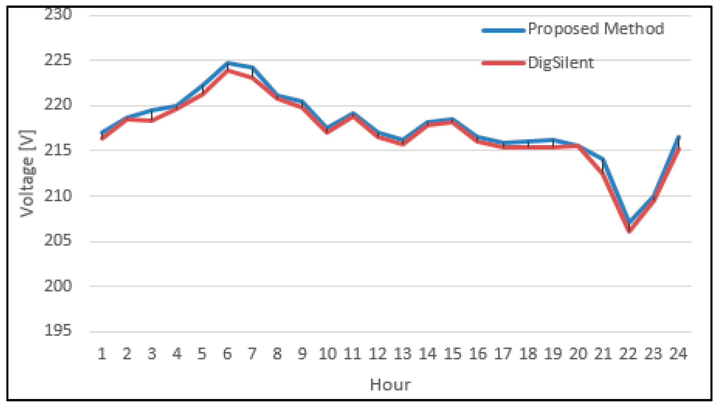
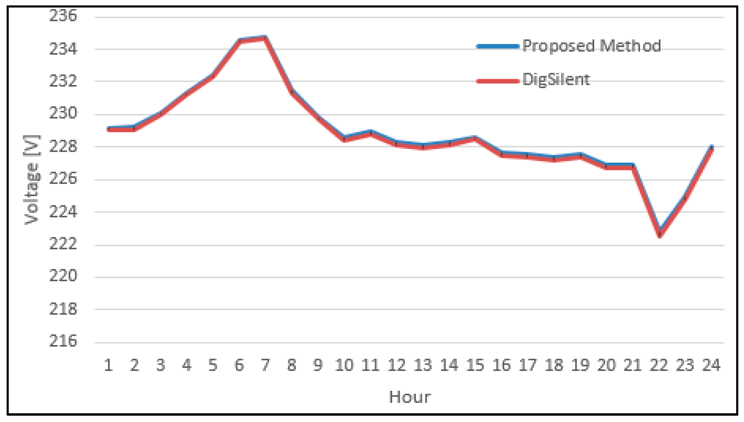
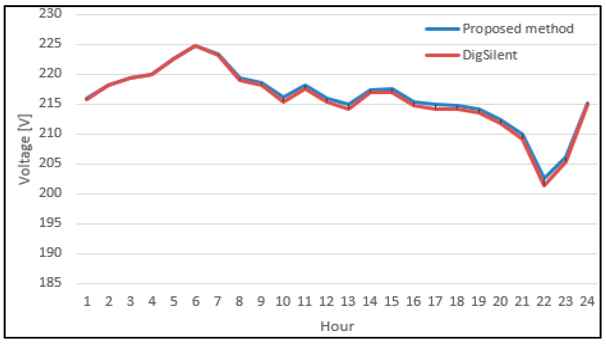
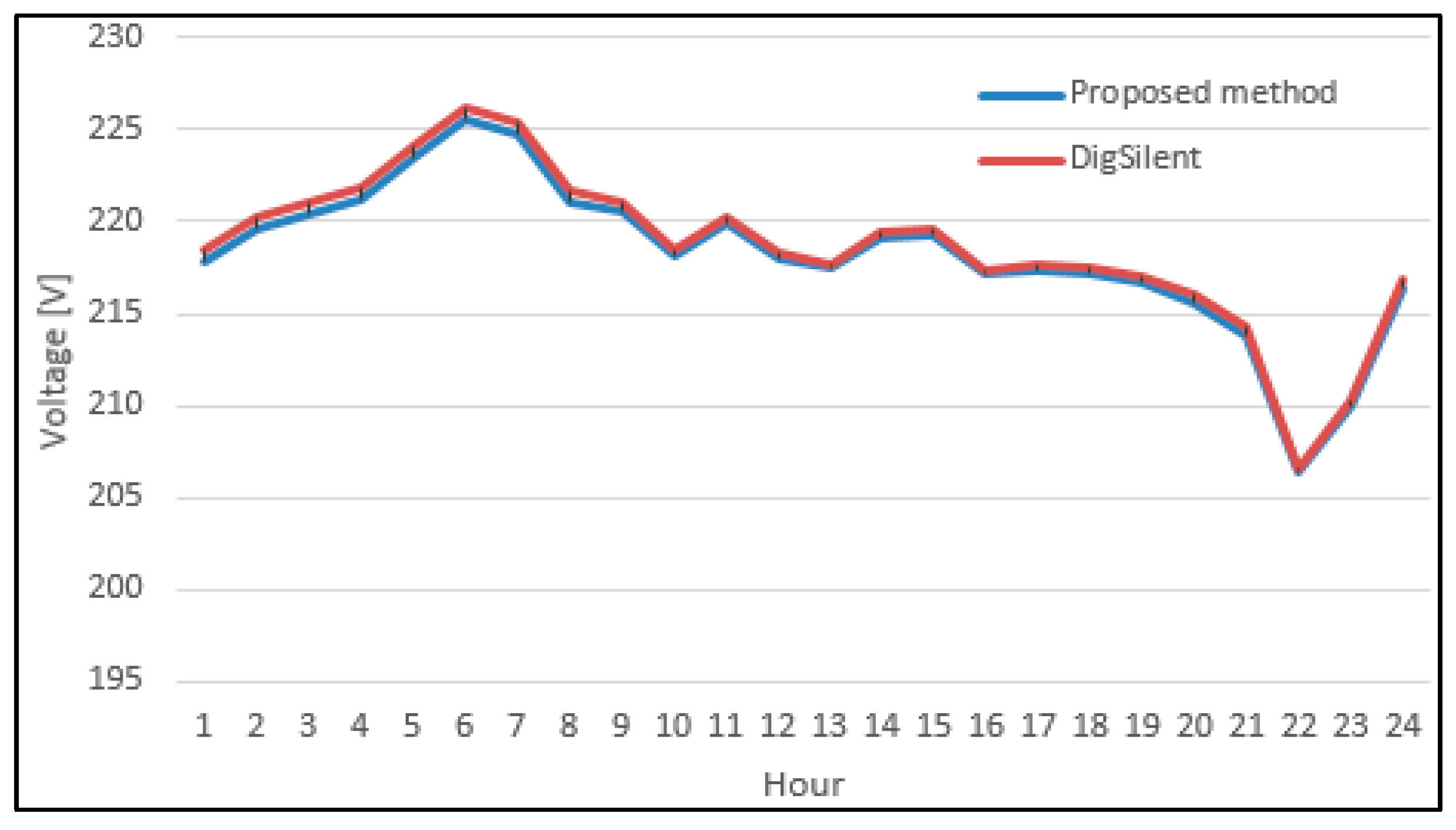
| Hour | Pillar P95 | Pillar P188 | ||||||||||
|---|---|---|---|---|---|---|---|---|---|---|---|---|
| PA | PFDS | PFDS | PFDS | |||||||||
| a | b | c | a | b | c | a | b | c | a | b | c | |
| 1 | 228.81 | 216.95 | 229.17 | 228.72 | 216.34 | 229.04 | 216.05 | 217.82 | 216.03 | 215.85 | 218.48 | 215.70 |
| 2 | 228.92 | 218.59 | 229.20 | 228.83 | 218.45 | 229.10 | 218.20 | 219.56 | 218.12 | 218.11 | 220.23 | 218.22 |
| 3 | 229.89 | 219.45 | 230.09 | 229.81 | 218.26 | 229.99 | 219.39 | 220.40 | 218.92 | 219.34 | 221.08 | 219.01 |
| 4 | 231.04 | 220.02 | 231.27 | 230.97 | 219.64 | 231.16 | 219.97 | 221.15 | 219.68 | 219.92 | 221.86 | 219.74 |
| 5 | 232.20 | 222.31 | 232.39 | 232.13 | 221.26 | 232.29 | 222.54 | 223.42 | 222.11 | 222.53 | 224.11 | 222.39 |
| 6 | 234.37 | 224.80 | 234.56 | 234.30 | 223.86 | 234.46 | 224.75 | 225.55 | 224.22 | 224.73 | 226.22 | 224.46 |
| 7 | 234.44 | 224.16 | 234.78 | 234.35 | 223.10 | 234.64 | 223.37 | 224.73 | 223.24 | 223.22 | 225.37 | 223.21 |
| 8 | 231.03 | 221.04 | 231.46 | 230.90 | 220.80 | 231.31 | 219.37 | 221.13 | 219.82 | 219.04 | 221.66 | 219.64 |
| 9 | 229.33 | 220.39 | 229.82 | 229.20 | 219.83 | 229.69 | 218.50 | 220.52 | 219.03 | 218.15 | 221.03 | 218.99 |
| 10 | 228.06 | 217.59 | 228.54 | 227.89 | 217.08 | 228.36 | 216.09 | 218.15 | 216.30 | 215.44 | 218.47 | 215.68 |
| 11 | 228.54 | 219.11 | 228.97 | 228.39 | 218.79 | 228.82 | 218.09 | 219.85 | 218.29 | 217.57 | 220.21 | 218.04 |
| 12 | 227.88 | 216.99 | 228.34 | 227.71 | 216.49 | 228.16 | 215.98 | 217.98 | 216.09 | 215.29 | 218.26 | 215.41 |
| 13 | 227.60 | 216.19 | 228.15 | 227.41 | 215.65 | 227.95 | 215.05 | 217.43 | 215.45 | 214.22 | 217.65 | 214.61 |
| 14 | 227.93 | 218.20 | 228.33 | 227.77 | 217.91 | 228.16 | 217.46 | 219.08 | 217.23 | 216.90 | 219.39 | 216.81 |
| 15 | 228.21 | 218.49 | 228.62 | 228.05 | 218.20 | 228.46 | 217.60 | 219.35 | 217.58 | 217.03 | 219.66 | 217.20 |
| 16 | 227.25 | 216.49 | 227.68 | 227.08 | 216.06 | 227.47 | 215.43 | 217.18 | 215.14 | 214.72 | 217.42 | 214.30 |
| 17 | 226.95 | 215.94 | 227.57 | 226.76 | 215.43 | 227.38 | 214.90 | 217.34 | 214.97 | 214.12 | 217.60 | 214.15 |
| 18 | 226.79 | 216.05 | 227.40 | 226.62 | 215.46 | 227.22 | 214.78 | 217.14 | 214.87 | 214.10 | 217.46 | 214.15 |
| 19 | 226.92 | 216.25 | 227.56 | 226.76 | 215.46 | 227.38 | 214.10 | 216.65 | 214.28 | 213.47 | 217.06 | 213.50 |
| 20 | 226.10 | 215.56 | 226.89 | 225.96 | 215.51 | 226.72 | 212.28 | 215.53 | 212.96 | 211.68 | 216.05 | 212.21 |
| 21 | 226.01 | 214.06 | 226.90 | 225.86 | 212.51 | 226.71 | 209.95 | 213.77 | 210.61 | 209.17 | 214.25 | 209.18 |
| 22 | 221.99 | 207.14 | 222.81 | 221.84 | 206.00 | 222.51 | 202.55 | 206.42 | 202.70 | 201.45 | 206.58 | 201.50 |
| 23 | 224.20 | 209.92 | 224.98 | 224.06 | 209.50 | 224.75 | 206.21 | 209.91 | 206.49 | 205.34 | 210.25 | 205.22 |
| 24 | 227.82 | 216.61 | 228.06 | 227.71 | 215.31 | 227.88 | 215.16 | 216.30 | 214.37 | 214.90 | 216.84 | 213.70 |
References
- Grigoras, G. Impact of smart meter implementation on saving electricity in distribution networks in Romania. In Application of Smart Grid Technologies. Case Studies in Saving Electricity in Different Parts of the World; Lamont, L.A., Sayigh, A., Eds.; Academic Press: Cambridge, MA, USA, 2018; pp. 313–346. [Google Scholar]
- Hierzinger, R.; Albu, M.; Van Elburg, H.; Scott, A.; Łazicki, A.; Penttinen, L.; Puente, F.; Sæle, H. European Smart Metering Landscape Report (IEE). 2013. Available online: https://ec.europa.eu/energy/intelligent/projects/sites/iee-projects/files/projects/documents/smartregions_landscape_report_2012_update_may_2013.pdf (accessed on 12 June 2019).
- Žádník, J. Cost Benefit Studies (CBA) for Smart Metering Roll-Out in the EU, Overview and Way Forward, Smart Grids in Practice. 29 September 2015. Available online: http://kampan.snt.sk/OSGP/prezentacie/PWC%202015_09_29_%20OSGP%20Slovakia%20Josef%20Zadnik.pdf (accessed on 12 June 2019).
- Institute of Communication & Computer Systems of the National Technical University of Athens ICCS- NTUA for European Commission. Study on Cost Benefit Analysis of in EU Member States Smart Metering Systems, Final Report. 25 June 2015. Available online: https://ec.europa.eu/energy/en/content/study-cost-benefit-analysis-smart-metering-systems-eu-member-states (accessed on 12 June 2019).
- European Commission. Smart Metering Deployment in the European Union. Available online: http://ses.jrc.ec.europa.eu/smart-metering-deployment-european-union (accessed on 12 June 2019).
- European Commission, Directorate-General for Energy. Standardization Mandate to CEN, CENELEC, and ETSI in the Field of Measuring Instruments for the Developing of an Open Architecture for Utility Meters Involving Communication Protocols Enabling Interoperability, M 441/EN. 2009. Available online: https://ec.europa.eu/energy/sites/ener/files/documents/2011_03_01_mandate_m490_en.pdf (accessed on 12 June 2019).
- European Commission, Directorate-General for Energy, Standardization Mandate to European Standardisation Organisations (ESOs) to Support European Smart Grid Deployment, M/490 EN. 2016. Available online: https://ec.europa.eu/energy/sites/ener/files/documents/2011_03_01_mandate_m490_en.pdf (accessed on 12 June 2019).
- Leonardo, M.; Queiroz, O.; Marcio, A.; Roselli, A.; Cavellucci, C.; Lyra, C. Energy Losses Estimation in Power Distribution Systems. IEEE Trans. Power Syst. 2012, 27, 1879–1887. [Google Scholar]
- Nassim, I.; Basa, A.; Çakir, B. A Simple Method to Estimate Power Losses in Distribution Networks. In Proceedings of the 10th International Conference on Electrical and Electronics Engineering (ELECO), Bursa, Turkey, 30 November–2 December 2017. [Google Scholar]
- Yusoff, M.; Busrah, A.; Mohamad, M.; Au, M.T. A Simplified Approach in Estimating Technical Losses in TNB Distribution Network Based on Load Profile and Feeder Characteristics. Recent Adv. Manag. Mark. Financ. 2010, 15, 99–105. [Google Scholar]
- Raesaar, P.; Tiigimagi, E.; Valtin, J. Strategy for Analysis of Loss Situation and Identification of Loss Sources in Electricity Distribution Networks. Oil Shale 2007, 24, 297–307. [Google Scholar]
- Bunluesak, K.; Horkierti, J.; Kaewtrakulpong, P. Power Loss Estimation in Distribution System A Case Study of PEA Central Area I. Available online: http://www.ecti-thailand.org/assets/papers/412_pub_24.pdf (accessed on 12 June 2019).
- Au, M.T.; Tan, C.H. Energy flow models for the estimation of technical losses in distribution network. In Proceedings of the 4th International Conference on Energy and Environment, Putrajaya, Malaysia, 5–6 March 2013. [Google Scholar]
- Feng, N.; Jianming, Y. Low-Voltage Distribution Network Theoretical Line Loss Calculation System Based on Dynamic Unbalance in Three Phrases. In Proceedings of the 2010 International Conference on Electrical and Control Engineering, Wuhan, China, 25–27 June 2010. [Google Scholar]
- Celli, G.; Natale, N.; Pilo, F.; Pisano, G.; Bignucolo, F.; Coppo, M.; Savio, A.; Turri, R.; Cerretti, A. Containment of power losses in LV networks with high penetration of distributed generation. CIRED Open Access Proc. J. 2017, 2017, 2183–2187. [Google Scholar] [CrossRef][Green Version]
- Mikic, O.M. Variance-based energy loss computation in low voltage distribution networks. IEEE Trans. Power Syst. 2017, 22, 179–187. [Google Scholar] [CrossRef]
- Ogunjuyigbe, A.S.O.; Ayodele, T.R.; Akinola, O.O. Impact of distributed generators on the power loss and voltage profile of sub-transmission network. J. Electr. Syst. Inf. Technol. 2016, 3, 94–107. [Google Scholar] [CrossRef]
- Zolkifri, N.I.; Gan, C.K.; Khamis, A.; Baharin, K.A.; Lada, M.Y. Impacts of residential solar photovoltaic systems on voltage unbalance and network losses. In Proceedings of the TENCON 2017—2017 IEEE Region 10 Conference, Penang, Malaysia, 5–8 November 2017. [Google Scholar]
- Gawlak, A.; Poniatowski, L. Power and energy losses in low-voltage overhead lines with prosumer microgeneration plants. In Proceedings of the 18th International Scientific Conference on Electric Power Engineering (EPE), Kouty nad Desnou, Czech Republic, 17–19 May 2017. [Google Scholar]
- Ramesh, L.; Chowdhury, S.P.; Chowdhury, S.; Natarajan, A.A.; Gaunt, C.T. Minimization of power loss in distribution networks by different techniques. Int. J. Electr. Power Energy Syst. Eng. 2009, 2, 1–6. [Google Scholar]
- Dashtaki, A.K.; Haghifam, M.R. A New Loss Estimation Method in Limited Data Electric Distribution Networks. IEEE Trans. Power Deliv. 2013, 28, 2194–2200. [Google Scholar] [CrossRef]
- Grigoras, G.; Cartina, G.; Istrate, M.; Rotaru, F. The Efficiency of the Clustering Techniques in the Energy Losses Evaluation from Distribution Networks. Int. J. Math. Models Methods Appl. Sci. 2011, 5, 133–141. [Google Scholar]
- Wang, S.; Dong, P.; Tian, Y. A Novel Method of Statistical Line Loss Estimation for Distribution Feeders Based on Feeder Cluster and Modified XGBoost. Energies 2017, 10, 2067. [Google Scholar] [CrossRef]
- Fernandes, C.M.M. Unbalance between Phases and Joule’s Losses in Low Voltage Electric Power Distribution. Available online: Fenix.tecnico.ulisboa.pt/downloadFile/395142112117/Resumo20Alargado%20Carlos%20Fernandes.pdf (accessed on 11 June 2019).
- Rupa, J.M.; Ganesh, S. Power flow analysis for radial distribution system using backward/forward sweep method. Int. J. Electr. Comput. Electron. Commun. Eng. 2014, 8, 1540–1544. [Google Scholar]
- Madjissembaye, N.; Muriithi, C.M.; Wekesa, C.W. Load Flow Analysis for Radial Distribution Networks Using Backward/Forward Sweep Method. J. Sustain. Res. Eng. 2017, 3, 82–87. [Google Scholar]
- Janecek, E.; Georgiev, D. Probabilistic extension of the backward/forward load flow analysis method. IEEE Trans. Power Syst. 2011, 27, 695–704. [Google Scholar] [CrossRef]
- Eremia, M.; Tristiu, I. Radial and Meshed Networks. In Electric Power Systems. Electric Networks; Eremia, M., Ed.; House of Romanian Academy: Bucharest, Romania, 2006; pp. 83–164. [Google Scholar]
- Grigoraș, G.; Gavrilaș, M. An Improved Approach for Energy Losses Calculation in Low Voltage Distribution Networks based on the Smart Meter Data. In Proceedings of the International Conference and Exposition on Electrical and Power Engineering (EPE), Iasi, Romania, 18–19 October 2018. [Google Scholar]
- Kriukov, A.; Vicol, B.; Gavrilas, M.; Ivanov, O. A Stochastic Method for Calculating Energy Losses in Low Voltage Distribution Networks Using Genetic Algorithms. AGIR Bull. 2012, 3, 595–602. [Google Scholar]


| Number of Reference | Objective Function | Online Estimation | Unbalanced Regime |
|---|---|---|---|
| [8,10,12,13,17,18,23] | Loss estimation using loss factor and load profile | No | No |
| [9] | Loss estimation using Elgerd’s power loss formulas | No | No |
| [11,19,20] | Joule Loss estimation | No | No |
| [14,24] | Loss estimation using load factor | No | Yes |
| [15,16] | Loss estimation using scaling factor for load profile | No | No |
| [21,22,24] | Loss estimation based peak load duration | No | No |
| [25,26,27,28] | Loss estimation using the backward/forward method | No | No |
| [28,29] | Loss estimation with losses factor, load factor and load profile | No | Yes |
| Number | Pillar | Branching | Phase | Type | Class | Integration | Meter ID |
|---|---|---|---|---|---|---|---|
| 1 | 1 | 1-P | b | 1 | 3 | 1 | 3002864374 |
| 2 | 2 | 1-P | b | 1 | 1 | 1 | 3002864354 |
| 3 | 2 | 1-P | c | 2 | 1 | 1 | 3002864393 |
| 4 | 3 | 3-P | abc | 1 | 1 | 1 | 3002864504 |
| - | - | - | - | - | - | - | - |
| N | 3 | 1-P | b | 1 | 1 | 1 | 3002108670 |
| VS1 | 1 | 2 | 3 | 4 | |||
| VS2 | I (1–2) | II (1–3) | III (3–4) | IV (4–5) | V (5–6) | VI (5–8) | VII (5–7) |
| Feeder | Length [m] | Conductor Type | Cross-section (Phase + Neutral) [mm2] | Length [m] | r0 [Ω/km] | x0 [Ω/km] |
|---|---|---|---|---|---|---|
| Feeder 1 | 280 | Classical | 1 × 50 + 50 | 280 | 0.61 | 0.298 |
| Feeder 2 | 3880 | Stranded | 3 × 35 + 35 | 120 | 0.871 | 0.055 |
| Classical | 3 × 50 + 50 | 3760 | 0.61 | 0.298 | ||
| Feeder 3 | 3520 | Stranded | 3 × 50 + 50 | 120 | 0.605 | 0.05 |
| Classical | 3 × 50 + 50 | 2080 | 0.61 | 0.298 | ||
| Classical | 3 × 35 + 35 | 960 | 0.871 | 0.055 | ||
| Classical | 1 × 25 + 25 | 280 | 1.235 | 0.319 | ||
| Classical | 1 × 16 + 25 | 80 | 1.235 | 0.319 | ||
| Total | 7680 | Classical | 7440 | |||
| Stranded | 240 |
| Consumers’ Type | 1-P | 3-P | |
|---|---|---|---|
| Phase a | 83 | - | |
| Phase b | 148 | - | |
| Phase c | 104 | - | |
| Total | 335 | 8 | |
| Consumption Class [kWh/year] | 0–400 | 150 | 5 |
| 400–1000 | 108 | 2 | |
| 1000–2500 | 65 | 0 | |
| 2500–3500 | 5 | 0 | |
| >3500 | 7 | 1 | |
| Feeder | Phase | Neutral | TOTAL | |||
|---|---|---|---|---|---|---|
| a | b | c | ||||
| Main conductors | Feeder 1 | 0.000 | 0.047 | 0.000 | 0.058 | 0.105 |
| Feeder 2 | 0.529 | 9.973 | 2.455 | 8.055 | 21.012 | |
| Feeder 3 | 6.370 | 5.411 | 5.726 | 1.586 | 19.092 | |
| TOTAL | 6.900 | 15.430 | 8.180 | 9.699 | 40.209 | |
| Branching conductors | Feeder 1 | 0.000 | 0.006 | 0.000 | 0.004 | 0.010 |
| Feeder 2 | 0.055 | 0.173 | 0.019 | 0.162 | 0.410 | |
| Feeder 3 | 0.072 | 0.052 | 0.052 | 0.086 | 0.263 | |
| TOTAL | 0.127 | 0.232 | 0.072 | 0.253 | 0.682 | |
| TOTAL | 7.026 | 15.662 | 8.252 | 9.951 | 40.892 | |
| Feeder | Phase | Neutral | TOTAL | |||
|---|---|---|---|---|---|---|
| a | b | c | ||||
| Main conductors | Feeder 1 | 0.000 | 0.043 | 0.000 | 0.054 | 0.097 |
| Feeder 2 | 0.509 | 9.647 | 2.433 | 7.765 | 20.354 | |
| Feeder 3 | 6.099 | 5.438 | 6.184 | 1.572 | 19.293 | |
| TOTAL | 6.608 | 15.129 | 8.616 | 9.391 | 39.744 | |
| Branching conductors | Feeder 1 | 0.000 | 0.006 | 0.000 | 0.004 | 0.010 |
| Feeder 2 | 0.053 | 0.218 | 0.020 | 0.187 | 0.479 | |
| Feeder 3 | 0.069 | 0.055 | 0.059 | 0.090 | 0.273 | |
| TOTAL | 0.122 | 0.279 | 0.079 | 0.281 | 0.762 | |
| TOTAL | 6.731 | 15.408 | 8.696 | 9.671 | 40.506 | |
| Approach | Phase | Neutral | Total | |||
|---|---|---|---|---|---|---|
| a | b | c | ||||
| PA | [kWh] | 7.03 | 15.66 | 8.25 | 9.95 | 40.89 |
| DSPF | [kWh] | 6.73 | 15.41 | 8.70 | 9.67 | 40.51 |
| ε | [kWh] | 0.3 | 0.25 | 0.45 | 0.28 | 0.38 |
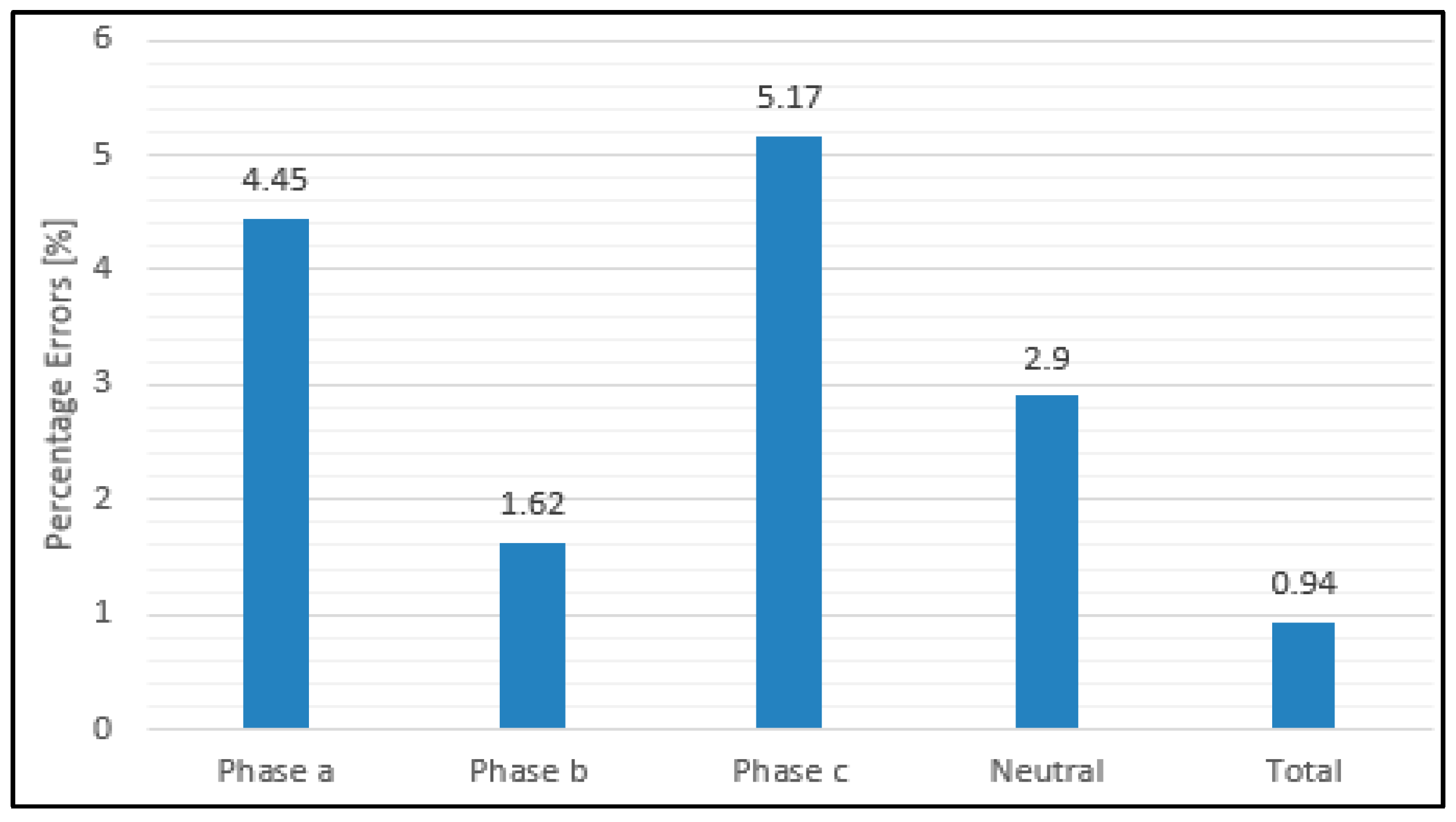
| δ | [%] | 4.45 | 1.62 | 5.17 | 2.90 | 0.94 |
© 2019 by the authors. Licensee MDPI, Basel, Switzerland. This article is an open access article distributed under the terms and conditions of the Creative Commons Attribution (CC BY) license (http://creativecommons.org/licenses/by/4.0/).
Share and Cite
Grigoras, G.; Neagu, B.-C. Smart Meter Data-Based Three-Stage Algorithm to Calculate Power and Energy Losses in Low Voltage Distribution Networks. Energies 2019, 12, 3008. https://doi.org/10.3390/en12153008
Grigoras G, Neagu B-C. Smart Meter Data-Based Three-Stage Algorithm to Calculate Power and Energy Losses in Low Voltage Distribution Networks. Energies. 2019; 12(15):3008. https://doi.org/10.3390/en12153008
Chicago/Turabian StyleGrigoras, Gheorghe, and Bogdan-Constantin Neagu. 2019. "Smart Meter Data-Based Three-Stage Algorithm to Calculate Power and Energy Losses in Low Voltage Distribution Networks" Energies 12, no. 15: 3008. https://doi.org/10.3390/en12153008
APA StyleGrigoras, G., & Neagu, B.-C. (2019). Smart Meter Data-Based Three-Stage Algorithm to Calculate Power and Energy Losses in Low Voltage Distribution Networks. Energies, 12(15), 3008. https://doi.org/10.3390/en12153008