1. Introduction
Thermal vacuum testing (TVT) is an important aspect of qualification testing for a wide variety of space-flight components, sub-assemblies, and mission-critical equipment. Space and upper atmospheric conditions, including temperature and altitude, can be simulated through TVT by removing air, reducing pressure, and cycling high and low temperatures. By testing in an environment that simulates real-world conditions as closely as possible, thermal vacuum exposure can identify design issues before they are integrated into larger systems, thus saving time and money.
Remarkable progress has been made in cryogenics in recent years. The increased operational reliability and simplicity of cryogenic equipment has allowed their installation and successful operation onboard spacecraft. At the same time, the improved performance of cryogenic devices, such as sensors and cold electronics, has drastically expanded their use, thus creating new perspectives for space-based applications [
1,
2,
3]. It is necessary to test all such components on the ground before launch, and accordingly, specific cold plates and cryostats need to be built and set-up.
Two main methods can be used to achieve cryogenic temperatures in vacuum conditions, namely cooling using refrigeration machines (cryocoolers) or cooling through heat exchangers by directly using fluids at cryogenic temperatures. Cryocoolers provide compact power capacities and an adjustable cooling power and temperature, and they do not require refurbishment. They are commonly used for the testing of small samples and devices (smaller than 500 mm) [
4,
5,
6,
7]. However, the main drawbacks of cryocoolers are high price, low efficiency for cooling large volumes, the induction of vibrations in the samples, and lower reliability. In contrast, cryogenic fluids, such as liquid nitrogen (LN
2) or liquid helium, can be used to cool large infrastructure systems or complex devices [
8] in a more efficient way when the temperature needed is similar to that of the cryogenic fluid. Moreover, cryogenic fluids are used as energy storage vectors [
9] and can cool samples without inducing external vibrations. Additionally, the mechanical system used for cooling is simply a passive heat exchanger, which leads to higher reliability and a lower price. However, continuous refurbishment is needed, since fluids boil off when cooling. Therefore, the choice of cooling method between cryocoolers or cryogenic fluids depends on the specific application and available resources.
Besides vacuum and cryogenic conditions, space components must also be tested under a controlled vibrating environment. This type of testing is normally conducted in a different test chamber, which increases the total cost of testing. Therefore, there is a significant interest in testing space components in vacuum, vibrating, and cryogenic conditions. Cryostats and cold plates for thermal and vacuum conditions have been widely developed by companies and research teams [
10,
11,
12,
13,
14]. However, the design of equipment for carrying out vacuum, cryogenic, and vibration tests simultaneously is not well developed.
This study proposes the use of a hexapod configuration to create a rigid and isostatic cold plate combined with a very good thermal isolation and the use of cryogenic liquid nitrogen to cool the plate down to −196 °C. The main contribution of this article is a design that has a unique set of properties: Simple construction, low thermal conduction, high thermal inertia, lack of vibrational noise when cooling, isostatic structural, high natural frequency, adjustable position, vacuum-suitability, reliability, non-magnetic and low cost. This design will permit the fast and low-cost manufacturing of ground-support equipment for testing space components at cryogenics.
This paper is organized as follows:
Section 2 describes the mechanical design, including the material selection criteria and technical drawings. Thermal and structural analyses are described in
Section 3. Manufacturing and assembly are outlined in
Section 4. Characterization test set-up is depicted in
Section 5. Experimental characterization results for vacuum, temperature, and vibrational behavior are listed in
Section 6. Finally, the main conclusions are listed in
Section 7.
2. Mechanical Design
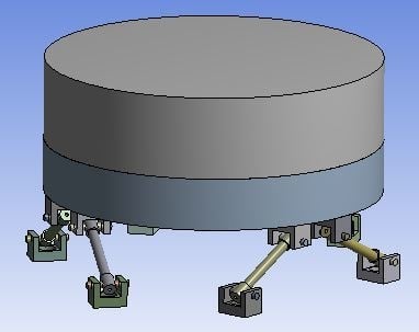
The cold plate design achieves the following requirements: Low thermal transfer, easy and low-cost manufacturing and assembly, the stability of position and orientation with temperature, good vibrational transmission (i.e., high natural frequency), and non-magnetic response. The hexapod configuration shown in
Figure 1 is proposed. This design consists of a vacuum-hermetic LN
2 cold vessel supported by six thermal isolating rods joined to a baseplate.
Each rod is connected to the vessel (or to the baseplate) through a hinge–axle–hole articulation. These articulations have three rotational degrees of freedom, leading to an isostatic construction. Since it layout is isostatic, this hexapod structure fulfills the structural requirements, avoiding any stress concentration due to misalignments or failures. Additionally, this hexapod structure has an easy assembly process and no cold plate reorientation or misalignments after cooling down.
In this type of articulated structure, linking rods bear only axial loads, thus avoiding the flexural movement of rods; this reduces the diameter of rod sections and reduces the thermal conduction of the rods. This is even more important in epoxy fiberglass elements, since they have an anisotropic elastic behavior due to the orientation of the glass fibers within the epoxy matrix. Another benefit of axial loading is that vibration mode frequencies are higher since the whole structure is more rigid.
2.1. Selection of Materials for Parts
In this design, the linking rods are the critical elements. The proposed design represents a tradeoff between high rigidity and low thermal conduction. In order to obtain the required rigidity with the minimum rod section, an analysis of material properties was conducted. Two main properties were considered, namely: The elastic modulus (E), whose variation with temperature is negligible; and thermal conductivity (k), whose variation with temperature is significant. Thermal conductivity values at cryogenic temperatures were obtained from the National Institute of Standards and Technology (NIST) database [
15]. As axial loads are only borne by rods, the parameter that defines the rods’ rigidity is the elastic modulus multiplied by the cross-sectional area (E·A). Thermal conduction depends directly on the thermal conductivity multiplied by the cross-sectional area (k·A). This parameter was set approximately equal for all the preselected material solutions by adjusting the outer and inner diameter of the cross-section. The E·A parameter was used as an indicator to determine which material has the best performance in terms of rigidity with similar thermal isolation capacity (k·A). The results of the tradeoff analysis are listed in
Table 1.
As shown in
Table 1, 304 stainless steel was found to offer the maximum rigidity for the same thermal isolation capacity. However, the required cross-section in stainless steel that fulfills the tradeoff is mechanically very difficult to produce, since machining a thread in such a thin tube is extremely complex. Therefore, epoxy fiberglass, which had the second-highest rigidity, was selected as the construction material for the six thermal isolating linking rods.
The vessel was made entirely of non-magnetic austenitic 316 stainless steel. A comparison between the characteristics of 304 and 316 stainless steel was performed. Though both materials are resistant against oxidation and corrosion, 304 stainless steel (which is by far the most popular of the 300-series of stainless steel) is not used in saline and water environments, since 316 stainless steel has superior resistance against corrosion and chemical attack. The magnetic permeability of both steels is negligible, although 316 has a slightly lower magnetic permeability than 304. Both have a content of 0.08% carbon, 2% manganese, 0.045% phosphorous, 0.03% sulphur, and 1% silicon. However, the lower content of chromium and higher content of nickel found in 316 stainless steel makes it appropriate for the current application.
The rest of the parts (hinges, axles, and acorn nuts) are not critical for the behavior of the cold plate. Accordingly, the selection of materials for these parts was based on material availability and manufacturing cost.
2.2. Assembly and Dimensions of Parts
The LN2 vessel is cylindrical with an external diameter of 200 mm and a total height of 138 mm. The vessel is made of two parts welded at the flange. Additionally, the top flange also has a welded DN16CF flange. A flexible bellow was used to join the LN2 vessel flange with the vacuum chamber lateral flange in order to transport LN2 into the vessel without vacuum leakages.
A grid of M6 screwed holes was drilled to attach the components being tested to the top of the vessel. Additionally, three deeper holes were made to allow for the fast cooling of some specific elements. These holes were directly immersed into LN
2. A schematic drawing of the vessel including the top and bottom parts is given in
Figure 2.
The vessel is supported by six linking rods, four of which are 60 mm length; the other two are 55 mm in length. A detailed schematic of the assembly, including linking rods, hinges, axles, and acorn nuts, is given in
Figure 3.
The linking rods were attached to the aluminum baseplate. The baseplate is 8 mm in thickness, and its sides had dimensions of 300 × 300 mm. For the cold plate, a grid of M6 screwed holes was drilled in the baseplate for the attachment of other elements such as sensors and actuators.
3. Thermal and Structural Analysis
In order to validate the material selection and design, different thermal and structural analyses was conducted. Details of the analysis models, assumptions, boundary conditions, loads, and results are described in this section.
3.1. Thermal Analysis
The main objectives of thermal analysis were (i) the determination of the temperature distribution on the cold plate (top surface of the LN2 vessel), (ii) the determination of the temperature along the linking rods, (iii) the estimation of the LN2 consumption needed to achieve and maintain the cold plate temperature, and (iv) the estimation of the time needed to reach operational temperature. To achieve these objectives, a nonlinear thermal finite element method (FEM) transient model was constructed using the ANSYS Structural Academic software v2019 R2 (Canonsburg, PA, USA).
3.1.1. FEM Model Geometry and Mesh
A 3D mechanical model was simplified in order to reduce the number of elements and to prevent divergence problems in critical areas. All screws, holes, and flange connections were removed. Additionally, the aluminum baseplate was removed, since the boundary conditions were applied directly to the bottom surface of the bottom hinges, assuming a steady-state in the baseplate. The simplified geometric model and its mesh are shown in
Figure 4. The mesh was generated using an automatic mesh generator feature in the ANSYS Structural Academic software with an element size of 0.0025 m. The mesh comprised 203,767 nodes and 112,721 tetrahedral elements. Convergence analysis of the mesh was performed in order to optimize the computation time and results. ANSYS structural automatic connections linked the elements of each part with the corresponding one.
3.1.2. Nonlinear Material Properties: Cp and k vs Temperature
In the cryogenic analysis and simulation, nonlinear heat capacity and thermal conductivity dependency must be considered. The property tables obtained from the NIST database were used for G-10 fiberglass epoxy, 316 stainless steel, and 6061-T6 aluminum. The values were extrapolated using curve-fitting equations of the following form:
where y represents the property, T is temperature in Kelvin, and the coefficients a, b, c, d, e, f, g, h, and i depend on each material and property. The coefficients used in the simulation are given in
Table 2.
3.1.3. Boundary Conditions, Thermal Loads and Analysis Settings
The temperature boundary conditions considered were room temperature and the bottom surface of the bottom hinges (22 °C-(A)) and the temperature of LN
2 at the bottom inner surface of the LN
2 vessel (−196 °C-(B)). The cold plate will always be used under vacuum conditions, and therefore the thermal loads applied in the simulation were intended to represent this operational environment. Radiation traveling from the outer surface of the vacuum chamber to the cold inner surfaces of the chamber was considered (D, E, F). For radiation, an external ambient temperature of 22 °C and emissivity according to the material were set. The following emissivities were considered: Anodized aluminum: ε
al = 0.7 [
16]; 304 stainless steel: ε
ss = 0.4 [
16]; and epoxy fiberglass: ε
ss = 0.85 [
17]. Two conditions were set inside the LN
2 vessel: (i) The bottom surface at −196 °C representing the liquid nitrogen phase and (ii) a convection flux applied to the lateral top surface representing the convection heat transfer from nitrogen gas evaporated from its liquid phase (G). The convection heat transfer coefficient for the nitrogen gas phase is 30 W/m
2 [
18]. The convection flux considers a heat transfer from walls to an ambient temperature of −196 °C, since evaporated nitrogen is at this temperature just after its evaporation. Finally, although the cold plate is in a vacuum environment, there is always some heat transfer due to residual gas particles. This gas conduction was measured in [
19] for a temperature difference from −196 °C to 22 °C for different values of vacuum residual pressure. Based on the figure on page 35 in [
19] and assuming a vacuum pressure of 10
−2 mbar, a heat flux of 29 W/m
2 from room temperature to colder parts was considered (C). In
Figure 5, colors and labels represent all thermal loads and boundary conditions.
Furthermore, transient analysis settings were adjusted to achieve sufficient accuracy with an affordable simulation time. The simulation parameters were as follows: The initial temperature was set in °C, the number of steps was 50, the step end time was 6000 s, the auto time stepping was set as “Program Controlled,” the initial time step was 1.2 s, the minimum time step was 0.12 s, the maximum time step was 12 s, and the time integration was set as “On.” All simulations were performed on a workstation with an Intel Core i5-7500 processor with 32 GB of RAM. With these conditions, the complete transient simulation lasted approximately 5 min.
3.1.4. Simulation Results
The results of the simulations described in
Section 3.1 are shown herein.
Figure 6 shows the simulated temperature distribution in all parts at the end time (i.e., after 6000 s of pouring LN
2 into the vessel). The results show that the average temperature on the top surface of the cold plate was −188.62 °C at the end of the simulation. The simulation results showed that the temperature distribution along the top surface of the cold plate varied within ±0.5 °C. Moreover, the results showed that the linking rods correctly isolated the LN
2 vessel from the baseplate, since the whole temperature gradient occurs in the rods.
Figure 7 shows the simulated temperature variation versus time. The variation of the temperature of the top surface had a sharped behavior between 0 and 250 s, and it became asymptotic at the end of the simulated time between 3500 and 6000 s. The temperature in the middle section of the linking rods decayed abruptly at the beginning of the simulation, while it reached an asymptotic value at −21.7 °C.
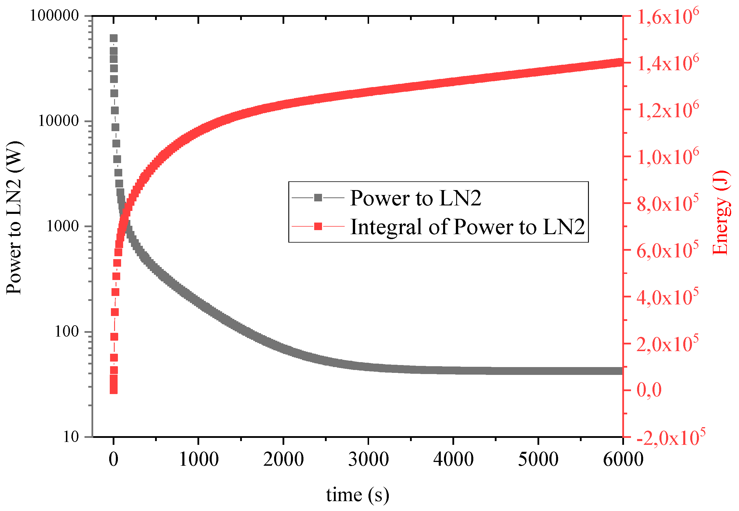
The simulation results show that the heat power transfer through the inner bottom surface of the LN
2 vessel can also be obtained. The simulated heat power versus time is shown in
Figure 8. The total spent energy with time was calculated by numerically integrating the heat power. The total energy transfer from LN
2 after 6000 s and the total LN
2 consumption can be determined by the following expression:
where 1403 kJ is the integral of the power and Q is the liquid nitrogen consumption. The value of 160 kJ/l is the evaporation enthalpy of LN
2. Hence, in order to achieve the operational temperature, 8.72 liters of liquid nitrogen are required.
The heat power asymptotic value was 42 W, which implies an LN2 flow of 0.9 L/h in order to maintain the operational temperature. Thus, this thermal analysis provides important information about the expected design behavior, which fulfills the requirements mentioned above.
3.2. Structural Analysis
The main objectives of the structural analysis were to determine the maximum vertical load capacity, vibration modes, and dynamic response. To accomplish these objectives, two structural FEM models were constructed, namely structural steady-state and modal harmonic analysis.
3.2.1. FEM Model Geometry and Mesh and Material Properties
The FEM model geometry is also a simplified version of 3D mechanical devices; indeed, it is the same geometry that is used in thermal analysis. We maintained the same mesh that was used in the thermal analysis. The automatic connection setting linked meshes of each part with the corresponding one. The cylindrical joint connection feature was used to connect acorn nuts with axles.
Though the elastic material properties change with temperature, the variations are lower than 10% according to NIST database. Therefore, constant elastic properties were assumed, and these are listed in
Table 3. The Young’s modulus of G-10 fiberglass epoxy was measured for checking in our labs, since this property can vary significantly depending on the fiberglass content of the samples.
3.2.2. Boundary Conditions, Structural Loads, and Analysis Settings
Boundary conditions for the structure were fixed support conditions at the bottom surface of the bottom hinges. For the structural steady state, a vertical load of 20 kN was applied to the baseplate. This shows that the hexapod structures can withstand very high loads when the rods are only loaded axially.
A vertical acceleration applied to the bottom surface of the bottom hinges was considered for modal harmonic analysis. The value of vertical acceleration was 1 m/s2, so the results are the transmissibility ratio. The harmonic analysis was performed between 0 and 250 Hz with 1 Hz intervals. The internal material damping was considered to be viscous and equal to 0.02 for all materials.
3.2.3. Simulation Results
The results of the steady-state simulation are shown in
Figure 9. The maximum equivalent stress predicted by the simulation was 444 MPa. This value is very close to the yield strength of epoxy fiberglass, which was found to be 448 MPa. Thus, this structure can withstand vertical loads of up to 20 kN.
Modal harmonic analysis was performed in two steps. The first step involved obtaining the first 10 vibrational modes of the structure, which are shown in
Table 4. The first and second main vibrational modes are found at around 85–90 Hz. These modes are rotational around an axis parallel to the top surface, as shown in the top of
Figure 10. Though these two modes generate vertical displacements in the borders of the top surface, the displacement in the center is null. In contrast, the third vibrational mode, found at 122.74 Hz, corresponds to uniform vertical displacements of the whole top surface; this mode is the most relevant, since accelerometers will be attached approximately at the center of the top surface. The bottom of
Figure 10 shows the deformation generated by this vibrational mode.
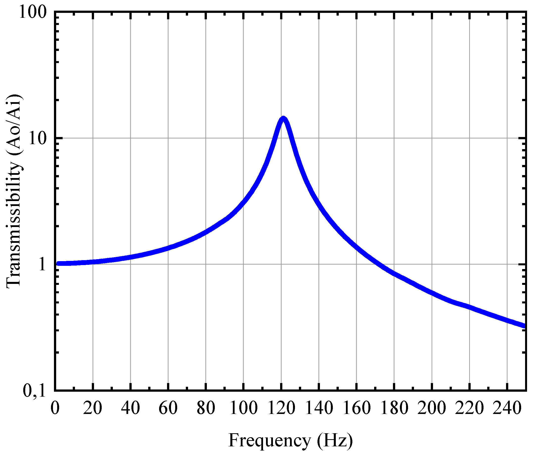
The second step of the simulation involves determining the frequency response of the vertical displacement of the cold plate. As shown in
Figure 11, a resonance of the vertical displacement was found at 122 Hz, as expected from the vibrational mode analysis.
4. Manufacturing and Assembly
The LN
2 vessel parts and baseplate were manufactured using an CNC OPTIMILL F105 machine from Optimum Maschinen Germany GmbH (Hallstadt, Germany) in the mechanical workshop of the University of Alcalá, Spain. Standard tools and a standard machine set-up for 304 stainless steel and 6061 aluminum were used.
Figure 12 shows photographs of some of the machined parts. The machining precision was lower than 50 µm.
The fitting between the top and bottom parts of the liquid vessel was 165 H7/e7. Such a reduced tolerance was obtained by progressively modifying the tool wear parameter on the CNC machine. Additionally, the connection flange DN16CF, which was made from 316 stainless steel, was produced by cutting a double DN16CF flange coupler from Kurt J Lesker Company (Jefferson Hills, PA, USA) for vacuum applications.
The linking rods were cut from an M6 threaded epoxy fiberglass rod with a length of 1 m provided by M.M. s.r.l. (Udine, Italy). The hinges, axles, and acorn nuts were purchased from external suppliers.
The top and bottom parts of the LN
2 vessel and the connection flange were welded together using a TIG welding machine with filler material for the build-up or reinforcement of the joints.
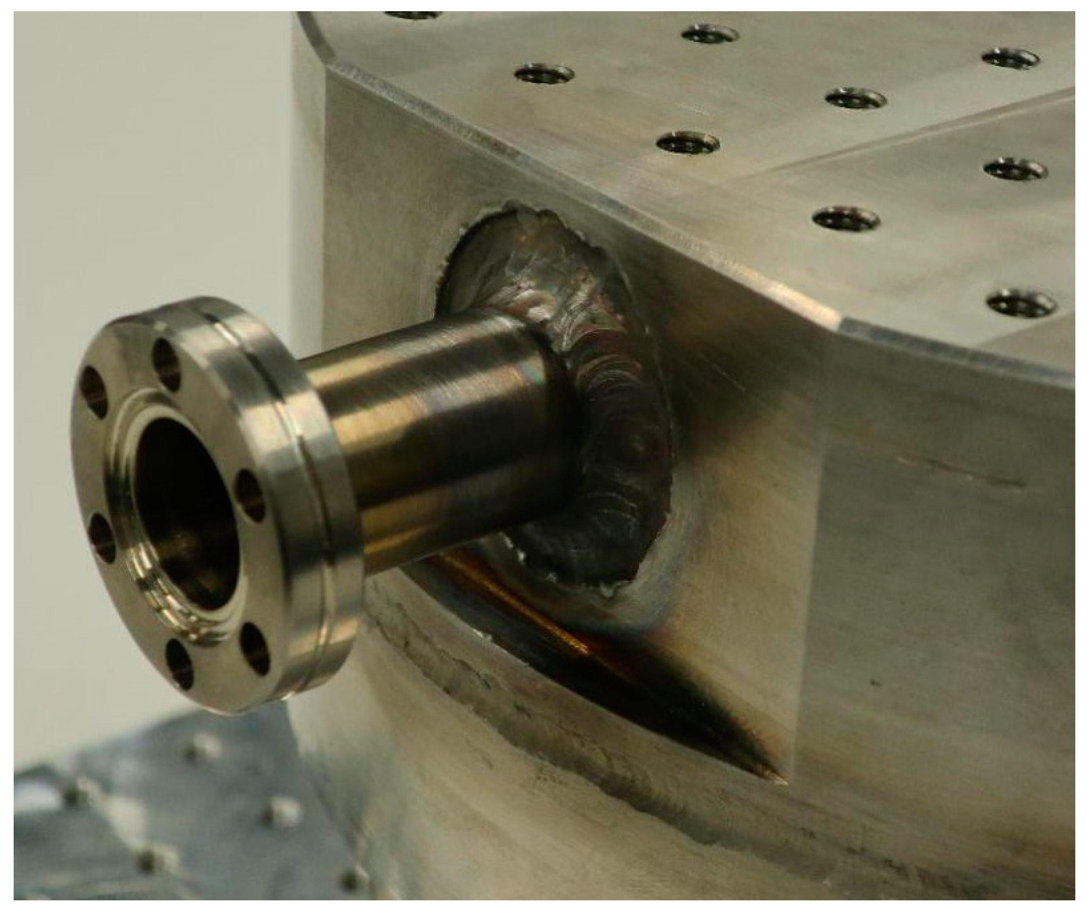
Figure 13 shows a photograph of the welding seams.
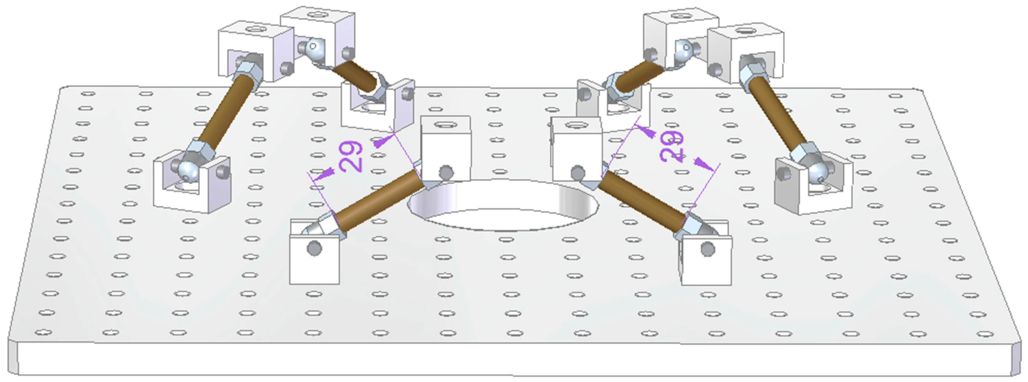
The whole assembly was done manually. The first step was to screw hinges to the baseplate and the bottom of the LN
2 vessel in the correct position for the final adjustment. The positions of the hinges are depicted in
Figure 14. Next, acorn nuts were connected to the hinges through axles. The acorn nuts were linked through a fiberglass M6 threaded rod.
When all the parts had been assembled, a final adjustment and alignment of the top of the cold plate was performed by threading the linking rods along the acorn nuts. Through this threading, the length of the epoxy fiberglass linking rods could be modified, and thus the top of the cold plate plane could be positioned and angularly oriented. The level and alignment of the top of the cold plate plane with respect to the baseplate was measured using a vertical caliper, obtaining a top plane maximum angular deviation of 0.5°. Once the cold plate had been correctly aligned and positioned, thread sealant was applied in the acorn nut and linking rod threads to maintain the selected adjustment. One interesting property of the hexapod configuration is that other orientations of the top of the cold plate plane could be obtained by simply modifying the distance between the linking rods and acorn nut threads.
Figure 15 shows some pictures of the complete structure after final assembly.
5. Test Set-Up
A test bench and sensing system were built in order to characterize the vacuum, thermal, and vibrational behavior of the cryogenic cold plate. The cold plate was mounted inside a cylindrical vacuum chamber. The useful size of the chamber is 500 mm in diameter and 210 mm in height. The chamber had six DN35CF flange type windows and one bottom flange connection for vacuum pumping. Two of the lateral windows were used as electrical pin port connections, and in another window, a KJLC (Jefferson Hills, PA, USA) cold cathode/Pirani combination gauge pressure able to measure pressures down to 10
−9 mbar was placed. The fourth window contained a manual vent valve. The fifth window was used as a port for four BNC coaxial wires. The last window was used to link with the external LN
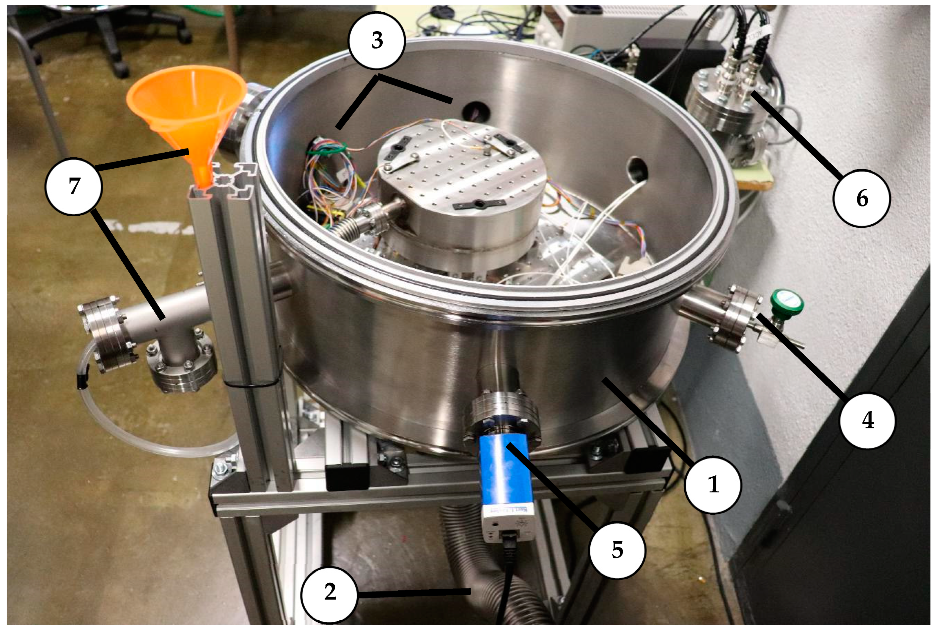
2 supply. The bottom flange was connected to a turbo-pump station with a turbo-molecular nEXT85H pump attached to an XDD1 dry diaphragm backing pump, both from Edwards (Burgess Hill, UK). A photograph of the cold plate inside the vacuum chamber test bench is shown in
Figure 16.
The LN
2 was supplied via a plastic pipe inserted into the vessel flange. In order to maintain a vacuum, the plastic pipe was surrounded by a flexible hermetic bellow screwed to the DN16CF LN
2 vessel flange. The other flange of the flexible bellow was connected to a customized DN16CF-DN35CF coupler screwed to the sixth window of the vacuum chamber, as shown in
Figure 17. The CF flange connections were all achieved by including a copper gasket, coated with vacuum-compatible grease, as a gap-filler between the flanges.
Three types of test can be conducted in the vacuum chamber, namely vacuum, thermal, and vibration tests. Vacuum tests were performed to demonstrate that the complete cold plate structure does not suffer additional vacuum leakages. Vacuum level versus time was registered for three operational conditions, namely empty chamber, cold plate inside chamber without LN2, and cold plate inside the chamber with LN2. The vacuum level was measured using the pressure gauge, and the pressure versus time was manually registered.
The objectives of the thermal tests were to verify that the desired temperatures were reached on the top surface of the cold plate and to determine the time and consumption of LN
2 necessary to achieve this temperature. Moreover, thermal tests allowed the FEM thermal model to be evaluated. The thermal tests were all performed from an initial vacuum condition and by pouring LN
2 inside the vessel. It was attempted to maintain a constant LN
2 flux in order to guarantee that at least the bottom part of the vessel was always at 77 K, as was set in the FEM model. Then, the temperature was measured using several PT100 platinum resistance probes connected in a four-wire configuration. Temperature measurements were made using a data acquisition system USB-6211 system from National Instruments (Austin, TX, USA) using a personal computer and the LabVIEW software from National Instruments. Four PT100 sensors were used: PT100-1, located at the baseplate; PT100-2, attached to a linking rod; and PT100-3 and PT100-4, placed at the cold plate. The PT100 sensors were encapsulated using Apiezon thermal-vacuum grease and an aluminum plate in order to guarantee the correct thermal contact. The exact positions of the PT100 sensors are shown in
Figure 18.
Vibration tests allow for the characterization of the dynamical response of the cold plate structure to external vibrational excitations. The accelerometers used were two IEPE 3035B uniaxial accelerometers (DYTRAN, Chatsworth, CA, USA) with a sensitivity of 100 mV/g, a frequency response of 0.5–10,000 Hz, and a mass of 2.5 g. The current source was an E4114B1 constant current power unit (DYTRAN) with an adjustable output current between 2 and 20 mA. External vibration excitations were applied using a 15 W electromagnetic shaker with an impedance of 8 Ω. One of the accelerometers was located on the bottom hinge in order to provide input acceleration measurement. The second accelerometer was attached to the surface of the cold plate surface. Acceleration measurements were made and treated using a 72-14535 EU digital oscilloscope (TENMA, Tokyo, Japan) with four channels, a bandwidth of 100 MHz, a sampling rate of 1 GSPS, and a memory depth of 28 Mpts.
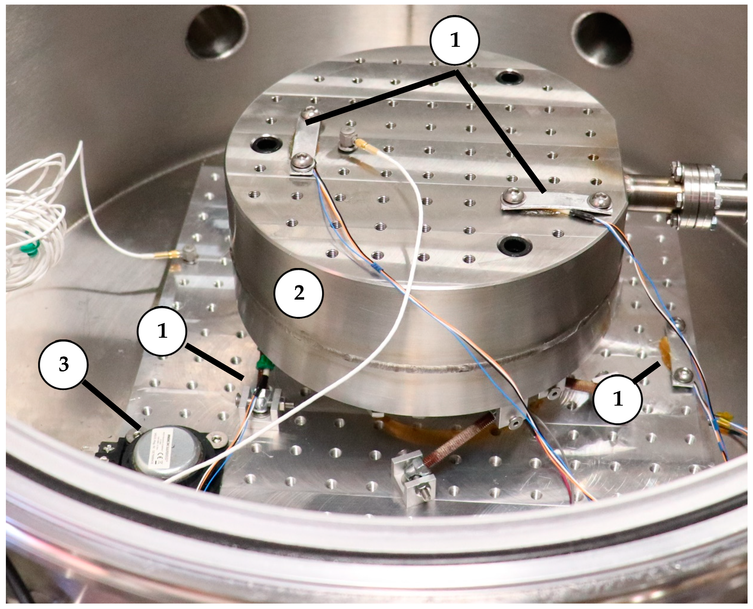
Figure 18 shows the locations of all the sensors mounted on the cold plate structure.
6. Experimental Results
Experimental tests were conducted to characterize and demonstrate the performance of the cold plate. Vacuum, thermal, and vibration tests were performed.
6.1. Vacuum Test
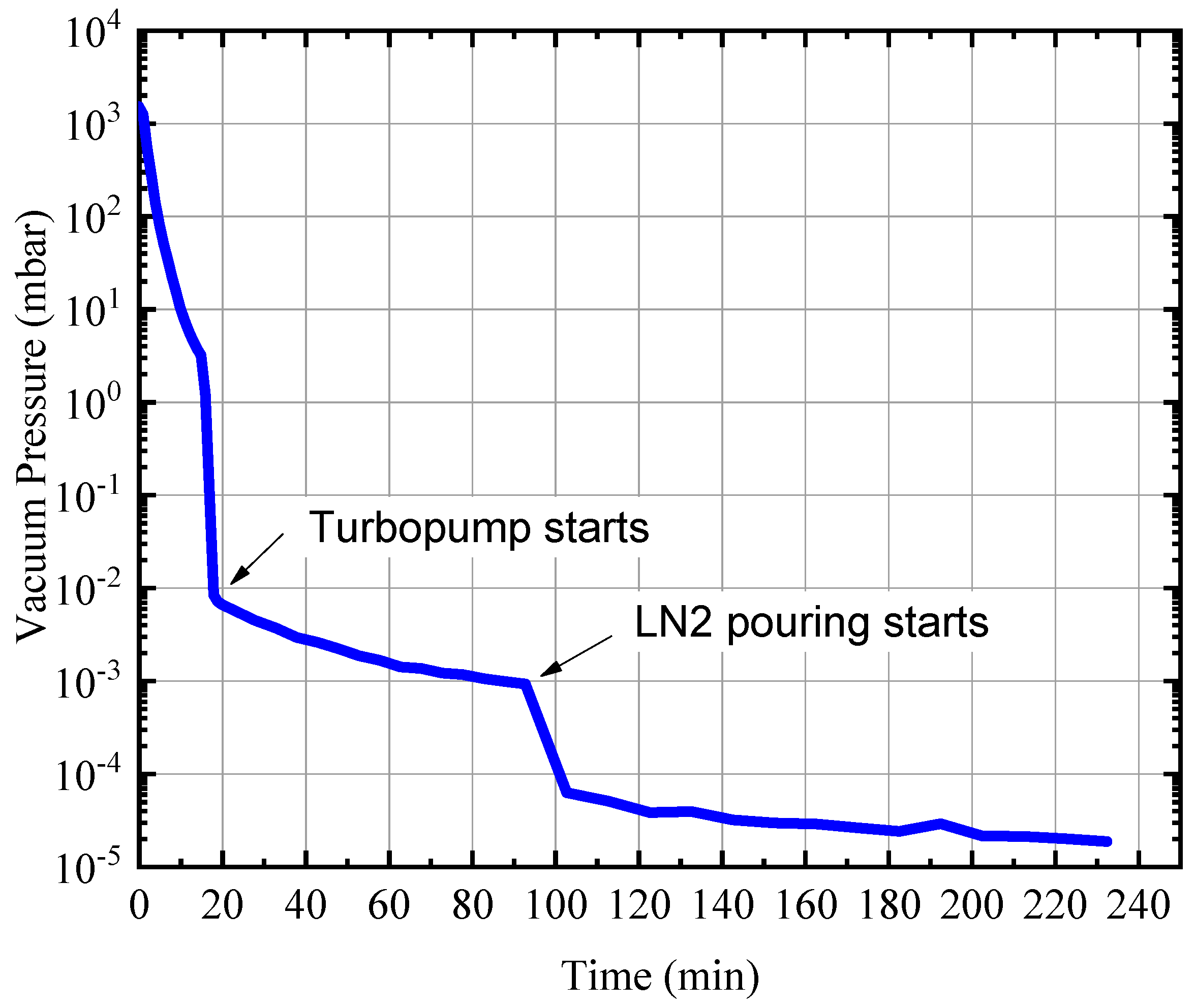
The vacuum pressure was registered over time. The results are plotted in
Figure 19. Air pumping was performed in three phases. During the first phase, the XDD1 dry diaphragm backing pump removed most of the air volume inside the chamber, reaching a vacuum level lower than 10
−2 mbar. After 15 minutes of pumping using the backing pump, the turbo-molecular pump and backing pump were activated simultaneously, reaching a free molecular regime inside the chamber. The stabilized vacuum level after turbo-pumping was measured at 10
−3 mbar. At this point, the third phase of vacuum production was started, with the pouring of LN
2 inside the vessel. The LN
2 vessel acted as a cold trap for the free molecular regime, significantly reducing the vacuum level to almost 10
−5 mbar.
Before assembling the cold plate inside the vacuum chamber, a similar vacuum pumping procedure was performed. Without the cold plate and associated connections, the measured vacuum level was 8 × 10
−4 mbar, which is on the same order as that measured in the vacuum test with the cold plate included, as shown in
Figure 19. Therefore, the cold plate does not induce undesired vacuum leakages. All seam welds were completely closed, and connection flanges operated correctly. Additionally, the cold plate can also be used as a cryogenic pump. The vacuum pressure achieved in this study was adequate to test mechanical and electronic devices for space applications.
6.2. Thermal Test
Thermal tests were initiated when a free molecular regime was achieved inside the vacuum chamber. At this point, LN
2 was continuously and manually poured into the vessel through a funnel and a plastic pipe. As shown in
Figure 20, the temperature on the surface of the cold plate started to decrease sharply from the very beginning of the pouring. After approximately 2000 s, the temperature on the cold plate was between −170 and −180 °C. Afterwards, the temperature decreased asymptotically towards its final stabilization temperature of −190 °C. During the beginning of the cooling process, there was a small difference between the temperatures measured by the two PT100 sensors placed on the cold plate. This is due to the fact that the PT100-4 sensor was closer to the LN
2 connection flange, which was cooled before the rest of the structure since the LN
2 entered from there. After 4000 s, the temperatures measured by the PT100-3 and PT100-4 sensors converged to −190 °C. The temperature in the linking rods stabilized at −19 °C after 2000 s of cooling. The temperature of the aluminum baseplate oscillated between 10 °C and 20 °C, which indicates that the thermal isolation was adequate. All this demonstrates that the cold plate can reach cryogenic operational temperatures and the hexapod structure effectively isolates thermal conduction.
A comparison between the simulated and measured temperatures is shown in
Figure 20. The simulated and measured temperatures on the cold plate are in very good agreement, with variations not larger than 10% during the cooling process. The variation between the simulated and measured final stabilized temperature was lower than 1.5%. Such a good agreement between the simulation and measurement was also observed for the temperature of the linking rod. This validates the thermal model and indirectly confirms the thermal cryogenic properties of the materials used for the construction of the structure.
Regarding the liquid nitrogen consumption, the simulations and measurements agreed less well than they did for temperature. In the physical test, a total of 10 L of LN2 was necessary to reach the final stabilized temperature after 6000 s of cooling, compared to the 8.73 l that were calculated using the simulation. This can be explained by the fact that neither the LN2 pouring pipe nor the funnel is totally adiabatic, leading to undesired heat power losses and LN2 evaporation. Additionally, LN2 replenishment was performed manually by using a small open LN2 vessel, which led to additional LN2 evaporation. Nevertheless, since 10 L of LN2 have a current cost of 2.5 €, the extra liquid required does not lead to a significant increase in the cost of the cooling.
6.3. Vibration Test
Additionally, the dynamic behavior of the cold plate hexapod structure was characterized. In
Figure 21, the vertical acceleration transmissibility curve is given together with the simulated behavior for comparison. The first acceleration resonance was found at 115 Hz. The difference between the measured and simulated values is 6%. This resonance is high enough for most vibrational tests of space components. Therefore, this cold plate design could be also used in vibrational tests of space components.
Both the simulated and measured vertical acceleration transmissibility curves reached the same peak value. This implies that the damping factor was correctly selected in the simulation analysis. However, the simulated and measured resonance frequencies are not the same: The simulated resonance frequency was 122 Hz while the measured one was 115 Hz. This 6% difference can be explained by the error in the simulation and the error in the measurement of the elastic properties of the epoxy fiberglass rods. Nevertheless, the simulated model reliably represented the dynamic behavior of the structure.
7. Conclusions
In the space industry, there is increasing demand for the designing and testing of components suitable for operation at cryogenic temperatures. In order to perform cryogenic validation tests, efficient and low-cost ground support equipment must be developed. In this study, we designed, manufactured, and tested a cold plate for the testing of cryogenic space components.
This article proposes the use of a hexapod configuration to create a cold plate. The proposed design has a unique set of properties: Simple construction, low thermal conduction, high thermal inertia, lack of vibrational noise when cooling, isostatic structural behavior, high natural frequency response, adjustable position, vacuum-suitability, reliability, non-magnetic, and low cost. The proposed design is presented as an alternative to expensive, noisy, and vibrating cryocoolers. In this article, the details of the design, manufacturing, and assembly of the cold plate are given, as are the thermal and dynamical models of the structure.
Successful characterization tests were performed to demonstrate the properties of the cold plate. Simulation models were also validated.
A vacuum test demonstrated that the cold plate does not add undesired vacuum leakages. The minimum vacuum level achieved was almost 10−5 mbar.
A thermal test showed that a cryogenic operational temperature of −190 °C can be reached on the top surface of the cold plate by pouring LN2 inside the vessel. Moreover, the structure demonstrated good thermal isolation between cold and hot parts.
Based on the vibration test, it can be determined that the structure is rigid and has a high resonance frequency, as desired. An acceleration resonance was found at 115 Hz. This resonance is high enough for most vibrational tests of space components. Thus, the designed cold plate could also be used in shaking vibration tests of space components.
Therefore, the presented cold plate has a high performance, is easy and cheap to replicate, and is useful for many tests of cryogenic space components.
Author Contributions
Conceptualization, E.D.-J.; methodology, E.D.-J. and E.P.; mechanical design, E.D.-J. and R.A.-S.; manufacturing and assembly, E.D.-J., R.A.-S., and P.M.V.; acquisition software, P.M.V.; validation test, E.D.-J., R.A.-S., and P.M.V.; formal analysis, E.P.; literature review, R.A.-S.; data curation, E.D.-J., R.A.-S., and M.J.G.G.; writing—original draft, R.A.-S. and M.J.G.G.; writing—review and editing, R.A.-S. and E.P.; supervision, E.D.-J.; project administration, E.D.-J.; funding acquisition, E.D.-J., and E.P.
Funding
The research leading to these results received funding from the Spanish Ministerio de Economía y Competitividad inside the Plan Estatal de I+D+I 2013–2016 under grant agreement n° ESP2015-72458-EXP.
Acknowledgments
The authors wish to recognize the work of Alba Martínez Pérez in the preparation of figures, the work of Miguel Fernández Muñoz in 3D model preparation, and the assistance of Hector Cruz Rosco during thermal and dynamic tests. The authors especially wish to recognize the work of Jorge Serena de Olano in CNC manufacturing.
Conflicts of Interest
The authors declare no conflict of interest.
References
- Collaudin, B.; Rando, N. Cryogenics in space: A review of the missions and of the technologies. Cryogenics 2000, 40, 797–819. [Google Scholar] [CrossRef]
- Pérez-Díaz, J.-L.; García-Prada, J.C.; Díez-Jiménez, E.; Valiente-Blanco, I.; Sander, B.; Timm, L.; Sánchez-García-Casarrubios, J.; Serrano, J.; Romera, F.; Argelaguet-Vilaseca, H.; et al. Non-contact linear slider for cryogenic environment. Mech. Mach. Theory 2012, 49, 308–314. [Google Scholar] [CrossRef]
- Valiente-Blanco, I.; Diez-Jimenez, E.; Pérez-Díaz, J.-L. Engineering and performance of a contactless linear slider based on superconducting magnetic levitation for precision positioning. Mechatronics 2013, 23, 1051–1060. [Google Scholar] [CrossRef]
- Pérez-Díaz, J.-L.; Diez-Jimenez, E.; Valiente-Blanco, I.; Cristache, C.; Sanchez-Garcia-Casarrubios, J.; Alvarez-Valenzuela, M.-A. Contactless Mechanical Components: Gears, Torque Limiters and Bearings. Machines 2014, 2, 312–324. [Google Scholar] [CrossRef]
- Valiente-Blanco, I.; Diez-Jimenez, E.; Sanchez-Garcia-Casarrubios, J.; Pérez-Díaz, J.-L. Improving Resolution and Run Outs of a Superconducting Noncontact Device for Precision Positioning. IEEE/ASME Trans. Mechatron. 2015, 20, 1992–1996. [Google Scholar] [CrossRef]
- Valiente-Blanco, I.; Pérez-Díaz, J.-L.; Diez-Jimenez, E. Dynamics of a Superconducting Linear Slider. J. Vib. Acoust. 2014. [Google Scholar] [CrossRef]
- Pérez-Díaz, J.-L.; Diez-Jimenez, E.; Valiente-Blanco, I.; Cristache, C.; Alvarez-Valenzuela, M.-A.; Sanchez-Garcia-Casarrubios, J.; Ferdeghini, C.; Canepa, F.; Hornig, W.; Carbone, G.; et al. Performance of Magnetic-Superconductor Non-Contact Harmonic Drive for Cryogenic Space Applications. Machines 2015, 3, 138–156. [Google Scholar] [CrossRef]
- Wang, Y.; Yang, G.; Zhu, X.; Li, X.; Ma, W. Electromagnetic Characteristics Analysis of a High-Temperature Superconducting Field-Modulation Double-Stator Machine with Stationary Seal. Energies 2018, 11, 1269. [Google Scholar] [CrossRef]
- Hamdy, S.; Moser, F.; Morosuk, T.; Tsatsaronis, G. Exergy-Based and Economic Evaluation of Liquefaction Processes for Cryogenics Energy Storage. Energies 2019, 12, 493. [Google Scholar] [CrossRef]
- Murray, A.J. Construction of a gravity-fed circulating liquid nitrogen dewar for experiments in high vacuum. Meas. Sci. Technol. 2001. [Google Scholar] [CrossRef]
- Swaffield, D.J.; Lewin, P.L.; Chen, G.; Swingler, S.G. Variable pressure and temperature liquid nitrogen cryostat for optical measurements with applied electric fields. Meas. Sci. Technol. 2004. [Google Scholar] [CrossRef]
- Boukeffa, D.; Boumaza, M.; Francois, M.-X.; Pellerin, S. Experimental and numerical analysis of heat losses in a liquid nitrogen cryostat. Appl. Therm. Eng. 2001, 21, 967–975. [Google Scholar] [CrossRef]
- Zhao, L.; Yang, Y.; Jing, J.; Qing, Y.; Gao, S.; Zhao, Y. New type of non-metal liquid nitrogen vessel for levitation system. IEEE Trans. Appl. Supercond. 2010, 20, 900–902. [Google Scholar] [CrossRef]
- Jiang, J.; Zhao, L.; Qin, G.; Yang, Y.; Qin, L.; Zhao, Z.; Zhang, Y.; Zhao, Y. Design and structural analysis of two kinds of liquid nitrogen vessel for high temperature superconductor maglev vehicle. IEEE Trans. Appl. Supercond. 2010, 20, 1896–1899. [Google Scholar] [CrossRef]
- NIST Cryogenic Materials Property Database Index. Available online: https://trc.nist.gov/cryogenics/materials/materialproperties.htm (accessed on 1 January 2019).
- Gubareff, G.G.; Janssen, J.E.; Torborg, R.H. Thermal Radiation Properties Survey; Honeywell Research Center: Wabash, IN, USA, 1960. [Google Scholar]
- Evertest Interscience Emissivity of Total Radiation for Various Metals. Available online: http://everestinterscience.com/info/emissivitytable.htm (accessed on 4 July 2019).
- Pusavec, F.; Lu, T.; Courbon, C.; Rech, J.; Aljancic, U.; Kopac, J.; Jawahir, I.S. Analysis of the influence of nitrogen phase and surface heat transfer coefficient on cryogenic machining performance. J. Mater. Process. Technol. 2016, 233, 19–28. [Google Scholar] [CrossRef]
- European Cryogenics Course-Cryogenic Thermal Insulators; Dresden University of Technology: Dresden, Germany, 2011.
Figure 1.
Mechanical design of the cold plate: (1) Aluminum baseplate; (2) aluminum hinges; (3) stainless-steel hollowed acorn nut; (4) fiberglass epoxy isolating rods; (5) liquid-nitrogen (LN2) vessel made from 316 stainless steel; (6) connection flange DN16CF made from 316 stainless steel.
Figure 1.
Mechanical design of the cold plate: (1) Aluminum baseplate; (2) aluminum hinges; (3) stainless-steel hollowed acorn nut; (4) fiberglass epoxy isolating rods; (5) liquid-nitrogen (LN2) vessel made from 316 stainless steel; (6) connection flange DN16CF made from 316 stainless steel.
Figure 2.
Technical drawing of the LN2 vessel: Top and bottom parts.
Figure 2.
Technical drawing of the LN2 vessel: Top and bottom parts.
Figure 3.
Schematic of the connecting rods.
Figure 3.
Schematic of the connecting rods.
Figure 4.
Simplified finite element method (FEM) model geometry and mesh.
Figure 4.
Simplified finite element method (FEM) model geometry and mesh.
Figure 5.
Boundary conditions and thermal loads (section plane view).
Figure 5.
Boundary conditions and thermal loads (section plane view).
Figure 6.
Temperature distribution in the whole structure (top), plane view and on the top surface of the structure (bottom).
Figure 6.
Temperature distribution in the whole structure (top), plane view and on the top surface of the structure (bottom).
Figure 7.
Simulated temperature variation versus time for top surface (averaged value) and for middle section element of one linking rod.
Figure 7.
Simulated temperature variation versus time for top surface (averaged value) and for middle section element of one linking rod.
Figure 8.
Heat power transferred to LN2 through the vessel inner bottom surface.
Figure 8.
Heat power transferred to LN2 through the vessel inner bottom surface.
Figure 9.
Structural steady-state simulation results: Maximum equivalent stress of 444 MPa.
Figure 9.
Structural steady-state simulation results: Maximum equivalent stress of 444 MPa.
Figure 10.
Vertical deformation of the first (top) and third (bottom) vibrational modes. The third mode is the most relevant for vertical deformations.
Figure 10.
Vertical deformation of the first (top) and third (bottom) vibrational modes. The third mode is the most relevant for vertical deformations.
Figure 11.
Vertical transmissibility (output acceleration (Ao) at the center of the cold-plate surface divided by input acceleration applied at the baseplate).
Figure 11.
Vertical transmissibility (output acceleration (Ao) at the center of the cold-plate surface divided by input acceleration applied at the baseplate).
Figure 12.
Bottom part of LN2 vessel (left), and baseplate (right), after machining.
Figure 12.
Bottom part of LN2 vessel (left), and baseplate (right), after machining.
Figure 13.
Detail of welding seams between the top and bottom parts of the LN2 vessel and between the top part of the LN2 and the connection flange.
Figure 13.
Detail of welding seams between the top and bottom parts of the LN2 vessel and between the top part of the LN2 and the connection flange.
Figure 14.
Positions of the hinges in the baseplate (left) and the bottom of the LN2 vessel (right).
Figure 14.
Positions of the hinges in the baseplate (left) and the bottom of the LN2 vessel (right).
Figure 15.
Complete structure after final assembly: Front (top) and lateral (bottom) views.
Figure 15.
Complete structure after final assembly: Front (top) and lateral (bottom) views.
Figure 16.
The cold plate inside the vacuum chamber: (1) Vacuum chamber, (2) pumping station bellow, (3) electrical pin ports, (4) manual vent, (5) pressure gauge, (6) BNC coaxial wire port, (7) LN2 supply.
Figure 16.
The cold plate inside the vacuum chamber: (1) Vacuum chamber, (2) pumping station bellow, (3) electrical pin ports, (4) manual vent, (5) pressure gauge, (6) BNC coaxial wire port, (7) LN2 supply.
Figure 17.
Connection to the internal LN2 supply through a flexible bellow (left). Connection to the external LN2 supply by direct pouring (right).
Figure 17.
Connection to the internal LN2 supply through a flexible bellow (left). Connection to the external LN2 supply by direct pouring (right).
Figure 18.
Sensors mounted on the cold plate structure: (1) PT100 temperature sensors, (2) vertically oriented accelerometers, and (3) an electromagnetic shaker.
Figure 18.
Sensors mounted on the cold plate structure: (1) PT100 temperature sensors, (2) vertically oriented accelerometers, and (3) an electromagnetic shaker.
Figure 19.
Air pressure inside the vacuum chamber versus time.
Figure 19.
Air pressure inside the vacuum chamber versus time.
Figure 20.
Experimentally measured and simulated temperatures.
Figure 20.
Experimentally measured and simulated temperatures.
Figure 21.
Measured and simulated vertical displacement transmissibility.
Figure 21.
Measured and simulated vertical displacement transmissibility.
Table 1.
Trade-off analysis: Rigidity versus thermal isolation.
Table 1.
Trade-off analysis: Rigidity versus thermal isolation.
| Material | Din (mm) | Dout (mm) | Area (mm2) | k (300 K) (W/mK) | k (77 K) (W/mK) | k (300 K)·A (Wmm2/mK) | k (77 K)·A (Wmm2/mK) | E (GPa) | EA (GPamm2) |
|---|
| Fiberglass epoxy | 0.00 | 6.20 | 30.19 | 0.60 | 0.26 | 18.11 | 7.85 | 3.50 | 105.67 |
| Carbonfiber Epoxy | 5.60 | 6.00 | 3.64 | 5.00 | 3.00 | 18.22 | 10.93 | 8.00 | 29.15 |
| Stainless Steel-304 | 5.87 | 6.00 | 1.26 | 15.00 | 6.00 | 18.87 | 7.55 | 200.00 | 251.61 |
| PTFE | 0.00 | 9.50 | 70.88 | 0.25 | 0.28 | 17.72 | 19.85 | 0.50 | 35.44 |
Table 2.
The curve-fitting coefficients used to calculate the thermal properties of various materials.
Table 2.
The curve-fitting coefficients used to calculate the thermal properties of various materials.
| Material | G-10 Fiberglass Epoxy | 316 Stainless Steel | 6061-T6 Aluminum |
|---|
| Coefficient | k (W/mK) | Cp (J/kgK) | k (W/mK) | Cp (J/kgK) | k (W/mK) | Cp (J/kgK) |
|---|
| a | −4.12360 | −2.408300 | −1.4087 | 12.2486 | 0.07918 | 46.6467 |
| b | 13.78800 | 7.600600 | 1.3982 | −80.6422 | 1.0957 | −314.2920 |
| c | −26.06800 | −8.298200 | 0.2543 | 218.7430 | −0.07277 | 866.6620 |
| d | 26.27200 | 7.330100 | −0.6260 | −308.8540 | 0.08084 | −1298.3000 |
| e | −14.66300 | −4.238600 | 0.2334 | 239.5296 | 0.02803 | 1162.2700 |
| f | 4.49540 | 1.429400 | 0.4256 | −89.9982 | −0.09464 | −637.7950 |
| g | −0.69050 | −0.243960 | −0.4658 | 3.1531 | 0.04179 | 210.3510 |
| h | 0.03970 | 0.015236 | 0.1650 | 8.44996 | −0.00571 | −38.3094 |
| I | 0 | 0 | −0.0199 | −1.9136 | 0 | 2.96344 |
Table 3.
Elastic properties of materials used in the structural simulation.
Table 3.
Elastic properties of materials used in the structural simulation.
| Material | G-10 Fiberglass Epoxy | 316 Stainless Steel | 6061-T6 Aluminum |
|---|
| Young’s modulus (GPa) | 3.5 | 200 | 71 |
| Poisson’s ratio | 0.3 | 0.3 | 0.33 |
| Shear modulus (GPa) | 12.5 | 76 | 26 |
Table 4.
The first 10 vibrational modes of the structure.
Table 4.
The first 10 vibrational modes of the structure.
| Mode | Frequency (Hz) | Mode | Frequency (Hz) |
|---|
| 1 | 85.82 | 6 | 231.09 |
| 2 | 90.64 | 7 | 1553.61 |
| 3 | 122.74 | 8 | 1554.01 |
| 4 | 184.47 | 9 | 1556.12 |
| 5 | 216.49 | 10 | 1559.3 |
© 2019 by the authors. Licensee MDPI, Basel, Switzerland. This article is an open access article distributed under the terms and conditions of the Creative Commons Attribution (CC BY) license (http://creativecommons.org/licenses/by/4.0/).

 ,
, 


