Abstract
The oil price time series data can be affected by major global political and economic events, which would result in structural changes that could lead to biased estimations. By adopting the Bai and Perron model this paper found that there were six structural breaks in the Brent oil price due to major global events and that ARDL-ECM cointegration exists only between oil price and stock market volatility index (VIX) throughout the sampling period. However, cointegration relations were found between oil price and Crude Oil Volatility Index (OVX) in the second and fourth sub-periods, and also between oil price and VIX in the second, third, fourth, sixth, and seventh sub-periods. Furthermore, the cointegration relation coupled with correlation analysis indicates a long-term equilibrium positive (negative) relation between the two variables. Such relations existed between the price and the two fear gauges, respectively, only for some specific sub-periods, implying that OVX seemed to be better than VIX in predicting oil price changes. We suggest that the investors in the global oil market must pay attention to not only the impacts of major global political and economic events on oil price, but also the positive or negative correlations between oil price and fear gauge.
1. Introduction
Many major political and economic events such as the overall economic impact [1], geopolitics [2], production capacity [3], supply and demand growth [4], speculative investment [5,6], European debt crisis [7], quantitative easing monetary policy [8,9], US exchange rate volatility [10,11], and crude oil inventory [12] tend to cause dramatic volatility in the prices in the global huge oil market. Meanwhile, these major global political and economic events can lead to structural changes to long-term economic behaviors [2,13,14,15,16,17]. It was found in the study by [18] that the major political or global events may cause structural changes to long-term time series data and that the inconsistency with the linear assumption would eliminate the cointegration relation between variables. Before that, [19] proposed a random transformation model which allowed change of trend line slope or level to test structural change. The results showed that there were potential permanent changes around the structural change points of energy events. Reference [20] employed the Ordinary Least Square Cumulative Sum (OLS-CUSUM) testing method with OLS residual to test the prices of the crude oil imported from Germany and found that oil price showed marked structural changes and its structural change points matched relevant major energy events. Reference [21] found that the negative relationship between oil price and global stock return was unstable and that there had been structural changes in oil price volatility since 2000. Previous methods of testing structural changes are incomplete because the time points of structural changes were not necessary for advance [22,23]. In other words, up to two structural change points can be tested in the series of exogenous variables [24]. In fact, there may be more than two structural change points due to the constant changes in the economic system. Therefore, if the multiple structural changes are not taken into account in the study, there will be errors in the results of the model test an increase in the probability of wrongly rejecting null hypotheses and incorrect explanation and inference [25].
In case of multiple structural changes of the time series data on long-term oil price, how investors use existing information or indexes about oil price to evaluate the direction of an oil price change and the length of time is an interesting topic in the study of oil price investing or hedging. As oil price volatility has a major influence on the global economy, some scholars have adopted relevant volatility indexes to measure the implied volatility of the price in the market to predict the change of oil price [26,27,28,29]. Traditionally, volatility is measured with the autoregressive conditional heteroskedasticity (ARCH) and Generalized autoRegressive conditional heteroskedasticity (GARCH) model (ex-post volatility) which is widely applied to historical price series [30]. The traditional GARCH model assumes that volatility remains unchanged, meaning the volatility of variables does not change with time [31]. However, neglecting these structural interruptions of the market may lead to a constantly fluctuating upward deviation, making it impossible to keep an accurate track of unconditional changes. This may cause the underestimation or overestimation of long-term volatility and thus weaken the prediction of the overall volatility in the market.
Relatively, implied volatility such as crude oil volatility index (OVX) and stock market volatility index (VIX) derives from option prices and can reflect the market’s prediction of the future volatility of option in the remaining period [2,7,32]. Some of the previous studies explored the relationship between implied volatility and the prices of various commodities. Reference [33] pointed out that there was not a long-term equilibrium relationship among the price of gold, the price of silver, exchange rate and the volatility index of the stock market VIX which takes risk perception as a driving factor of a long-term oil price. Reference [34] studied the relationship among VIX, the dollar index, and oil price and found that VIX had a spillover effect on oil price; meanwhile, the dramatic change of dollar index led to combined change with an increase in the uncertainty of oil price. Reference [35] explored the volatility and conditional correlation among oil price, the price of gold and the price of the bond and found that in most cases petroleum was the best hedge asset for the stock in emerging markets and VIX or bond was the most effective hedge tool for the stock in emerging markets. Reference [36] used the implied volatility index (VIX) provided by Chicago Board Options Exchange (CBOE) to explore the relationship between oil price and the American energy stock market and found that there was a long-term relationship between oil price and the implied volatility index of the stock market (VIX). The causality test shows that there was a short-term leading effect between the implied volatility of global petroleum and the American energy stock market.
Reference [37] argued that VIX, which was used to measure the risk aversion benchmark, could not be directly applied to the test on the volatility of the petroleum market because the crude oil future market included a complicated and diversified trader structure; they adopted the uncertainty of the petroleum market and the OVX of the new derivatives to predict the market’s prediction of the price volatility of crude oil in the following 30 days. Earlier, reference [7] studied the relationship between OVX and other implied indexes and found that there was not a long-term equilibrium relationship between them but there was short-term cross-market uncertainty transmission effect between petroleum and other major markets.
Reference [38] found that the relationship between oil price and its volatility index (OVX) played a key role in all kinds of transactions. Reference [39] tested the information about OVX and pointed out that OVX could make more effective the prediction of volatility. Reference [40] argued that there is a negative but asymmetrically contemporaneous relationship between the change of OVX and the returns of crude oil. Reference [41] believed that OVX had a negative impact (implied volatility impact) on Chinese stock indexes and five industrial stock returns. But after the global financial crisis, the influence of OVX on the actual volatility of the Chinese stock market has been greatly reduced.
Reference [37] documented that there was a significantly negative relationship between OVX change and US West Texas Intermediate price of oil (WTI) returns during the sampling period, and the asymmetric relationship in the period indicated that OVX index (rather than risk preference) was more effective in prediction to measure the fear of investors. Reference [42] introduced newly implied volatility indexes (OVX, VIX, and GARCH) to study the correlation between petroleum price and share prices in the eleven major security exchanges over the world from 2008 to 2015. They found that the relationship between petroleum and equity had the two-way informational spillover effect in the two markets and most of the transactions were shifted from the petroleum market to the stock market.
Additionally, there have been studies on the correlation between OVX and VIX in recent years. For instance, [43] found that the uncertainty of the petroleum market had a substantial impact on the actual volatility of the markets in most cases; even if the effects of S&P500 implied volatility indexes (VIX) were controlled, OVX still influenced about half of the stock markets in the Middle East and Africa. Reference [44] examined the dynamic analysis on which CBOE adopted three volatility indexes, namely VIX, OVX and gold price volatility index (GVZ), to explore the implied volatility transmission of inter-market correlation. Reference [45] used five implied volatility indexes including VIX, OVX, euro/dollar exchange rate volatility index (EVZ), GVZ and treasury note volatility Index (TYVIX) to test the correlation among them and found that the correlation changed with time during the period of economic and financial instability.
In summary, whether the long-term and short-term dynamic relationship between oil price and OVX (VIX) changes due to major global events is a hot topic on the study of structural change. That is, if the problem of structural changes existed, has it changed the dynamic relationship between oil price and OVX (VIX)? To date, few studies have been done on this topic; this paper is filling in the blank. Therefore, this paper aims to investigate what caused multiple structural changes, how the structural changes affected the oil price behavior, and what relationships existed between oil price and the two fear gauges (OVX and VIX) of investors, reflecting oil price volatility under multiple structural changes. Besides, feasible suggestions are provided for the investors in investment and hedge decisions in the global petroleum market.
2. Research Methods
This paper investigates empirically the long-term and short-term dynamic relationships between oil price, OVX, and VIX under structural changes. First, this paper employed the structural change testing model by [25,46,47] to test the structural change of oil price over the sampling period, including the date and confidence interval of structural change points. Second, it used the autoregressive distributed lag and error correction item (ARDL-ECM) by [48] to test the long-term equilibrium relationship between the price and two fear gauges (OVX vs. VIX). Finally, statistical correlation techniques were adopted to analyze the correlation between the price and the two fear gauges.
2.1. Structural Change Model
Recalling the previous studies relating to the structural changes, [19,23] showed that the possible locations of change points be confirmed before the model set. The unit root test by [49] under structural change would cause problems in confining given points of structural change. Reference [50] converted the unit root test of structural change of given points into the unit root test on unknown points and allowed the estimation of the locations of structural change points. Reference [51] considered a time point of structural change endogenously determined by the model itself. Reference [52] solved the problem of identifying given change points, but only a single structural change point could be obtained, which leads to a reduction of the testing power for time series data under multiple structural changes. References [46,53] presented a modified technique to find the mean and trend of multiple structural change points. But the empirical study by [24] found that the method by [53] could be used to effectively find out structural change points. Reference [25] indicated that many major events would have jumping impacts on overall economic variables, thus developing a unit root test that extended the structural change of an unknown point to the structural change of two unknown points.
With the suppose of several change points in the time series data, [47] further extended the sum of squared residuals (Sum of squared residuals, SSR) to estimate the number and location of structural change points of the mean equation. References [25,46,47] proposed four sequential procedure methods for structural change points (see the Appendix A of this paper). This method not only analyzed time series having several structural change points but also estimated the number of structural change points. The Sequential procedure method by [25,47] is described briefly as follows:
Reference [46] adopted the SSR to estimate if there were structural change points of variables in the linear model. Suppose that the linear regression model of variable yt which has m structural change points in the m + 1 intervals is specified by:
where yt is the dependent variable of the t-th period; xt and zt are the vectors of (p × 1) and (q × 1), respectively; and are the corresponding parameter vectors; (j = l, ..., m, +1, ) is the moderation variable of the tth period; (T1, T2, …, Tm) is an unknown structural change point in the model. If the parameter vector of in Equation (1) is invariant, then it is called a partial structural change model; if p = 0, it is called a pure structural change model. All the parameters ( and ) in the m + 1 intervals (T1, T2, … Tm) is estimated with SSR:
Let and be the regression parameter estimates of the m + 1 intervals (T1, …Tm), and substitute them into the objective function of Equation (2). Let SSR be and substitute it into the following equation to obtain the estimate equation for structural change points:
Equation (3) indicates that each interval has the minimum SSR; the regression parameter estimate is correlated with the m + 1 intervals; each interval has its own estimate. Therefore, if m ≥ 2, the method can be used for estimation.
After the parameter estimate of the structural change model is obtained, several procedures can be used for the hypothesis testing on the estimates of structural change points. In the operational procedure where no change points are detected and there is only one change point, the ability to detect SupFT (i = 1) is weak, which would cause the incorrect estimation that there are no change points. Hence, SupFT (i = 2) is adopted to test rejecting the null hypothesis without change points. Finally, the sequential procedure is used: SupFT (l + 1|l) is adopted to determine the number of structural change points until rejecting the null hypothesis. However, the model does not have a constraint on structural change points; hence, there may be more than one structural change point (as for the two methods of applying BIC and LWZ to estimate the number of structural change points, please see the studies by [54,55]).
To examine the number and date of the time points of structural changes, this paper adopted the method by [25,47] and combined two testing methods SupFT (i) and SupFT (l + 1|l). Moreover, 10% of trimming (trimming parameter, ) is used to set up to eight structural change points, and the errors in cross-section residuals are allowed to be correlated with the series of different variables. The first F testing method SupFT (i) is a structural change test where the null hypothesis is 0 and the opposite hypothesis is i, i refers to 1, …, 8, indicating that there is at least one and up to eight structural change points under the 5% significance level; if i = 2 in the opposite hypothesis, the statistical value will be the highest. The second F testing method SupFT (l + 1|l) is the sequential testing method. The null hypothesis has l structural change points, and the opposite hypothesis has l + 1 structural change points. This method aims to test the opposite hypothesis of a single change point of (l + 1) in comparison with the null hypothesis of no structural change point. This method can be applied to each period which covers such estimate change points as i − 1 and i (i = 1, …, l + 1). If the global minimum of least squared residual (including the sum of all periods of additional change points) is fully lower than the sum of least squared residuals of a change point model, then the null hypothesis with (l + 1) change points will be rejected. The selected date of change point is the one related to the global minimum. i − 1 estimate does not need to be the minimum of global squared residual; we can use this sets of methods to test if it meets the above conditions period by period to determine the number of change points.
2.2. ARDL-ECM Cointegration Model
This paper analyzes the long-term equilibrium relationship between oil price and OVX and VIX, respectively. If it is impossible to confirm if the dependent variable or independent variable is I(0) or I(1), this paper follows the suggestions by [56] and adopts the error correction items involving variables to explore the long-term equilibrium relationship among these variables. This will solve the problem of inconsistency of integration orders of time series data. [48] took a further step by proposing the (ARDL-ECM) which included intercept item, time trend item and error correction item. The equations of the model are as follows:
where OP is oil price; OVX refers to oil volatility index; VIX is the volatility index of stock index option; is an intercept item; indicates the slope of time trend item; represents white noise; p refers to the lag period number of the difference of dependent variables; q is the lag period number of the difference of independent variables, which is represented by ARDL(p, q). Additionally, the ARDL(p, q) model is categorized as three sub-models: Model 1 is the one with no intercept and no trend ; Model 2 is the one with intercept and no trend ; Model 3 is the one with intercept and trend .
According to [43], this paper adopted two independent statistics to determine the existence of long-term relationship: the F test () on the joint significance of the coefficients in the lag period and the t-test () on the null hypothesis in Equation (4) or Equation (5). If the independent variable is I(d) (), the boundary between two asymptotic critical values provides the cointegration test, which assumes that the lower limit of the independent variable is I(0) and the upper limit is I(1). If the F value of the test statistic exceeds the upper limit, there will be a long-term equilibrium co-integration between two variables; if the test statistic is lower than the lower limit, the null hypothesis of cointegration will be rejected; if the test statistic is between the upper and lower limits, it will be impossible to make a judgment. There are three advantages in using ARDL-ECM to analyze the cointegration among variables: (1) it is unnecessary to consider if the integration orders of variables are the same; (2) it can strengthen the test power of small number of samples; (3) it is possible to identify dependent and independent variables themselves [48]. However, there are two limitations regarding the use of the ARDL bounds test. As stated above, if the F value is between the upper limit and lower limit, whether to accept or reject the null is inconclusive so that this test cannot be used. In addition, the use of this test is inappropriate if the time series data shows nonlinear characteristics [57].
3. Empirical Result and Analysis
To explore the impacts of global political and economic events on oil price, we used two fear gauges (OVX vs. VIX) to test if a higher fear gauge caused by major global events would cause dramatic oil price changes. That is, is there a cointegrating relationship between oil price and the two fear gauges, respectively? And is their relationship positive or negative? This paper focuses empirically on all these issues.
3.1. Data Source
The data used in this study include Brent crude oil price, VIX, and OVX, which are collected from the economic database of Federal Reserve Bank of St. Louis covering from 10 May 2007, to 13 November 2017 (2639 observations included). According to the definition by the CBOE, VIX is the volatility index consisting of S&P500 index options rather than stocks, and the price of each option reflects the market’s prediction of volatility in the coming 30 days. OVX is used to calculate the crude oil ETF volatility index of Limited Partnership (LP) option in the CBOE transactions according to the USO (LP option refers to a limited partner option transacted in the CBOE in the name of USO); the CBOE merely includes the standard (due in the third Friday) option series in the VIX calculation, with OVX and VIX sharing the same calculation method. Concerning literature on VIX or OVX, refer to [38,58], etc.
Reference [7] indicated that OVX is an indicator to measure the volatility of the crude oil price which can directly predict the oil price volatility in the coming 30 days. A VIX value higher than 40 represents that investors begin to feel upset about the future trend of stock price indexes, and one lower than 15 implies an increasingly stable market. According to Table 1, the standard deviation of OVX is higher than that of VIX, which means that VOX is greatly volatile. Except that the skewness of oil price is negative and leftward biased, those of both OVX and VIX are rightward biased. This indicates that oil price remains stable for most of the time in the entire sample period. Except that the kurtosis of oil price is 1.73 and shows platy kurtosis that of both OVX and VIX are higher than 3 and show leptokurtosis. Jarque-Bera (J-B) values also confirmed that OVX and VIX rejected the normality of the null hypothesis.

Table 1.
Descriptive Statistics.
According to Figure 1a,b, Brent oil prices exhibited a negative relation with OVX and VIX, respectively, for most of the time. In other words, if OVX and VIX declined, the oil price would register a stable rise, but during the full sample observation period, there seem to be several dramatic structural change trends. These might be associated with the major global political and economic events at that time.
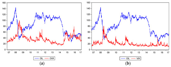
Figure 1.
(a) Oil Price and OVX. (b) Oil Price and VIX.
3.2. Analysis of Structural Changes
3.2.1. Number and Date of the Structural Change
On the first and second columns of Table 2, when the number of structural changes of oil price is tested, successive SupFT (l + 1|l) testing statistics cannot reject the null hypothesis of l = 1 structural change point according to the two sequential procedure methods, SupFT(i) and SupFT(l + 1|l). This means that it is impossible to accept only one structural change point at the 5% significance level; instead, the testing must be continued until the null hypothesis without structural change point is rejected. Therefore, the null hypothesis is still continuously rejected in case of l = 1, l = 2, …, l = 6 in this paper, and the null hypothesis without structural change point is accepted when l = 7. In other words, the testing results of l = 6 are significant; hence, we conclude that there are six structural change points in the entire sampling period. Bayesian information criterion Bayesian information criterion (BIC) and the modified Schwarz criterion (LWZ) proposed by [55] are used according to the suggestion by [54], and we find that BIC and LWZ are the minima when the number of structural change points is 6. This result is identical to that of the Sequential procedure methods (if this paper adopts the double maximum testing method, the results will be as follows: it will be impossible to get the specific date of structural change point; the number of structural change points will be greatly different from that obtained with the above three methods. Therefore, the results obtained with this method are not shown in this paper.).
Table 2.
Results of Test on Structural Changes of Oil Price.
Following the suggestion proposed by [25], this paper adopted two sequential procedure methods, SupFT(i) and SupFT(l + 1|l), to determine the number of structural change points and indicate the changes that exceed 10% ( of regression mean. The tested dates are 8 October 2008, 23 October 2009, 11 January 2011, 19 March 2013, 13 November 2014, and 16 December 2015, respectively. Figure 2 shows the regression means the process of oil price and the dates of structural change.
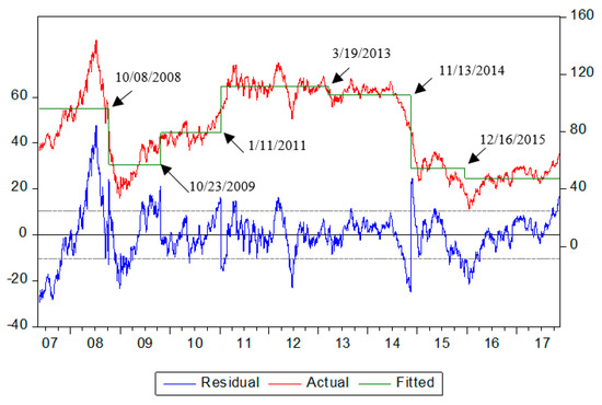
Figure 2.
Regression Mean Process of Oil Price and Dates of Structural Changes.
According to the literature, Organization of the Petroleum Exporting Countries (OPEC) production reduction agreement, the stock market, dollar exchange rate, speculation, gold market, geopolitics, and climate are all the supply-demand factors which influence oil price fluctuations. The crude oil pricing mechanism is rather complicated, and the final price is often the outcome of the combined effects of the above forces. According to the overall change of oil price, once there is a structural change to the path of oil price fluctuation, it usually means that an influencing factor plays a key role in the middle- and long-term period and may substitute or influence the petroleum exporting countries’ future pricing mechanism.
According to the above six structural change points (as is shown in Table 2), we divided the entire sampling period (10 May 2007~13 November 2017) into seven sub-periods.
3.2.2. ARDL-ECM Cointegration Analysis
According to [18], the results of cointegration test on structural change show that as some long-term time series data go against the assumption of time-invariant linear combination, there may not be a cointegrating relationship between variables for the model set of different levels and trends and different testing statistics.
As time series data may be time-variant in structural change and it is unnecessary to consider if the integration orders of variables are consistent, this paper adopted the ARDL-ECM proposed by [43] to test if there is a cointegrating relationship between variables. After confirming the structural change of oil price, this paper employed the ARDL-ECM to find that there is not a cointegrating relationship between oil price and OVX in the entire sampling period (10 May 2007~13 November 2017) but there is a cointegrating relationship between oil price and VIX (as is shown in Table 3 Panel A, Model 3). For the seven sub-periods, in Table 3 Panel B, there is not a cointegrating relationship between two variables in the first sub-period (10 May 2007~7 October 2008), but there is one (Model 2 and Model 3) in the second sub-period (8 October 2008~22 October 2009). There is a cointegrating relationship (Model 3) between oil price and VIX in the third sub-period (23 October 2009~10 January 2011); there is one (Model 2) between two variables in the fourth sub-period (11 January 2011~18 March 2013); there is not one between two variables in the fifth sub-period (19 March 2013~12 November 2014); there is a cointegrating relationship (Model 1) between oil price and VIX in the sixth sub-period (13 November 2014~15 December 2015) and one (Model 2 and Model 3) in the seventh sub-period (16 December 2015~13 November 2017). The results of the cointegration analysis in this study are the same as that of the study by Gregory and Hansen [18]. In other words, the structural change would change the original long-term equilibrium relationship between two variables.
Table 3.
Results of ARDL-ECM Cointegration Test.
3.3. Correlation Analysis
According to the long-term trend of oil price, the global oil price stayed between USD 22 and 30 before the US-Iraq War in the last ten days of March 2003, and oil price suddenly soared after the outbreak of the war. One month later, Iraq was defeated in the war, and the situation in the Middle East became stable, and the oil price returned to the level of USD 23 to 25. After that, the US government began to adopt a low-interest rates easing policy to stimulate the economic recovery of the US and the world. Major industrial countries had an increasing demand for petroleum, which once again gradually drove up to the oil price. Through the global financial crisis in the middle of September 2008, the oil price had risen up to more than USD 140. As the investors in the global oil market had become used to the over-supply on petroleum, the oil price showed a long-term rise; nevertheless, as they suddenly became confronted with the American subprime mortgage crisis and the subsequent global financial crisis and the Fed immediately adopted the quantitative easing monetary policies, the two fear gauges (OVX and VIX) reflect the anxiety about oil price rise swiftly. [59] further indicated that there do not exist significant price bubbles in the Brent oil during the period over 2003–2008, and the main driver of oil price boom is fundamentals. Therefore, there is a positive relationship (Table 4: Correlation Analysis; the coefficient of correlation between OVX and oil price is 0.718, and that between VIX and oil price is 0.157) between the rise of oil price and rising fear gauges in the first sub-period (10 May 2007~7 October 2008). During the period, the oil price rose from USD 64.63 to USD 80.77; OVX climbed from 27.09 to 62.6; VIX rose from 13.6 to 57.53. This empirical result is identical to that of the study by [35].
Table 4.
Correlation between variables.
The observation on the remaining sub-periods shows that there is a negative relationship between oil price and the two fear gauges, respectively. This is the same as the results of the previous studies [2,21,37,40,60].
According to further analysis, the global stock market was seriously hit since the collapse of Lehman Brothers since September 2008 in the second sub-period (8 October 2008~22 October 2009). The pressure of the continuous decline of financial asset resulted in the reduction of risk preference. Then, the Fed adopted the Quantitative Easing policy (QE1), which resulted in the structural change to VIX. Moreover, the OPEC reached the petroleum production reduction agreement in advance. All these drove both VIX and OVX to rise quickly [7]. Nevertheless, the pessimistic attitude towards economic prospect has triggered greater uncertainty in the future economic outlook, increased the worry about global economic growth, and enhanced the pressure of oil price decline. This means that these major impacts on structural changes to oil price have led to the trend that oil price dropped and then rose, which indicates a negative relation with the trend of the two fear gauges that first rose and then dropped (the correlation coefficient between OVX and oil price is −0.752, and that between VIX and oil price is −0.533). The result of this sub-period in this study is very similar to [2] in that there is a significantly negative relationship between oil price and OVX.
During the third sub-period (23 October 2009~10 January 2011), Iran’s nuclear program led to greater tension in the Middle East, and the prediction that the OPEC would increase the demand for oil drove the oil price to climb. The financial crisis and the European debt hit the oil price again, but after the strike in France, the US Fed announced continued QE2 and positive news about the overall economic situation. During the sub-period, the oil price showed the trend of first declining and then dramatically rising, and the two fear gauges first climbed and then dropped. The reason is that after the rising oil price led to higher fear gauges before November 2009, the investors predicted that the oil price would continue to stay high for a long time. Reference [61] pointed out that after the second break, the pressure on dollar depreciation since the implementation of QE2 in December 2010 gradually increased, and a tremendous amount of dollar funds were shifted from the US into the speculative crude oil markets, which made oil prices rise to a new high since the financial tsunami. Therefore, the slight fall of the oil price in the current period unexpectedly led to a sudden increase in the fear of investors and rising fear gauges. Nonetheless, as global political and economic situations became tense and the oil price rose again, the investors believed that it was natural that the oil price would stay high for a long time, which led to the decline of fear gauges. Hence, there was a significant negative relationship between the oil price trend and the fear gauges during the sub-period (the correlation coefficient between OVX and oil price was −0.715, and that between VIX and oil price was −0.625). Similarly, Reference [59] documented that in the Brent crude oil prices of the period over 2009–2011, the self-reinforced behaviors caused by the non-linear positive feedbacks are fairly weak; that is, there do not exist significant bubbles; instead, the main driver of the growth of Brent crude oil prices is fundamentals.
During the fourth sub-period (11 January 2011~18 March 2013), the dollar continued to depreciate, and there were conflicts in North Africa and the Middle East. The Jasmine Revolution continued to develop; the US economic recovery became sluggish; the debt crisis in the Eurozone appeared again; there was pressure of rising interest rate and volatility in the global exchange rate; the US public debt rating declined, and the Fed’s QE policy remained at a super-low interest rate, and dollar depreciated again. All these pushed the oil price to USD 123.5. Meanwhile, the US economy became sluggish, without any solution to the fiscal deficit, and China began to adopt a deflationary monetary policy to restrain inflation. Moreover, China set a new low record in PMI, and the oil price continued to decline to a record low. Afterward, there was the news that Iran faced the trade sanction from Western countries due to its development of nuclear weapons, which fueled the increase in the oil price; the EU Summit put forward the strategies to tackle the European debt. After that, the risk interference of geopolitics, the Fed’s QE3 and other favorable factors contributed to the continued volatility of oil price at a high rank. After that, the Fed announced the launch of the QE4 policy, and the geopolitical interference didn’t disappear. As a result, the oil price rose slightly. In 2013, both the US and Mainland China witnessed eye-catching economic performance; the American fiscal crisis was alleviated; there were frequent outbreaks of geopolitical conflicts in the Middle East and North Africa. All these accelerated the rise of the oil price. During the sub-period, the oil price trend was influenced by the complicated global political and economic factors. Although the fear gauges dropped slightly, the correlation between the two variables was not significant (the correlation coefficient between OVX and oil price was −0.179, and that between VIX and oil price was −0.171). Compared with [54], the results of this study show that except for the fundamentals driving the Brent oil price, the geopolitical factor also plays an important role for the price dynamics, whose result is the same as [62] during this sub-period.
During the fifth sub-period (19 March 2013~12 November 2014), the IMF adjusted the global economic growth rate in 2013, and China and the US faced sluggish economies, which enhanced the oil price restraint pressure, but Japan released QE and the re-occurrence of geopolitical turmoil kept the oil price from declining and making it stable. The European Central Bank lowered the benchmark interest rate and the US employment market continued to stay stable. This drove the oil price to go up, but the global supply of oil was stable, the European economy remained sluggish, and the market predicted that the Fed would reduce QE. All these offset the above favorable factors and caused the oil price to merely stay between USD 100 to 110. After that, the situations in the Middle East and North Africa became tense; the US registered remarkable economic growth, and the commercial crude oil inventory continued to shrink; both Europe and the US witnessed positive manufacturing indexes. All these resulted in a higher oil price. Later, Iran’s nuclear problem was alleviated; Fed probably shrank QE; the geopolitical risk in the Middle East and North Africa was reduced; the US consumer confidence indexes fell short of expectations, which led to restraint in the oil price. Only the fact that the Fed announced the persistence in the existing QE enabled the oil price to stay at a relatively high level. Subsequently, the Fed announced that it would curtail QE by USD 100-750 after January 2014, and China’s economy became sluggish. This caused the pressure on the oil price to decline. In general, the oil price faced serious hit and increased the fear among the investors during the period, hence, there was a medium negative correlation between oil price and OVX (the correlation coefficient was −0.557), but as the US, Japan, and the EU continued to implement quantitatively loose monetary policies and there were adequate funds in the supply market, the stock market showed signs of stability and rose, revealing a relatively stable VIX trend of fear gauges in the stock market. Therefore, there was an insignificant relationship between oil price and VIX (the correlation coefficient was −0.290). The results of this study are consistent with [54] in that the fundamentals (demand and supply) are the main drivers of the Brent and WTI oil prices during this sub-period.
During the sixth sub-period (13 November 2014~15 December 2015), the Iraqi government reached an agreement on the income distribution of crude oil exporting with Kurds; the production of the crude oil in the US reached a new height since 1983, the US Department of Commerce announced the confirmatory principles for condensed oil exports. All these led to a lower oil price, but later, the armed conflict in Libya deteriorated, Nigeria’s crude oil exporting schedule was dramatically cut, and the US witnessed a better economic situation. These helped stop the drop in the oil price. Reference [63] documented that during the fifth break in December 2014, the European Central Bank conducted a number of easing policies and the issue of independence in Scotland has driven the US dollar to strengthen, and the oil price has fallen even more. But in 2015, the US crude oil inventory increased; Saudi Arabia and Iraq continued to lower the price; the IMF once again lowered the expectations for global economic growth and the anti-austerity faction won the Greek parliamentary elections. These factors changed the market direction, and Brent price declined to USD 50. Afterward, major oil-producing countries like Libya and the United Arab Emirates suffered attacks on their oilfields and facilities; the workers of US refineries went on a strike, and the number of idle crude oil drilling machines in the US climbed; many large oil companies released news about reducing staff and capital expenses. Then, the decline of the oil price finally came to a halt. The European Central Bank announced that the debt purchase plan with a monthly payment of EUR 60 billion would be put into reality since March. However, Saudi Arabia raised export quotas; the turmoil in Libya became worse, which threatened the country’s oilfields, oil ports, and airports; a fierce conflict broke out in Yemen, which drove the United Arab Emirates to launch air attacks and other geopolitical volatility. Iran reached an agreement on its nuclear weapons, and the oil embargo on the country was removed, but as the IEA predicted that the production of shale oil in the US would decline and raised the predicted value of global petroleum demand, the oil price stopped dropping and bounced back. The conflicts in the oil ports in eastern Libya, the deteriorating geopolitical conflict in Iraq where IS controlled the provincial capitals, the shrinking US commercial crude oil inventory, and the ever smaller number of crude oil drilling machines in the operation pushed the oil price to keep rising. The OPEC continued to set the same production target; the negotiations between Iran and P5+1 were smooth; Greece encountered a debt crisis once again. All these led to an ever lower oil price. However, Greece’s poor repayment, the collapse of the Chinese stock market and other bad economic news cast a layer of uncertainty over the prospective demand and fueled the decline of the oil price. Despite China’s less demand for crude oil, the US FOMC’s maintaining the interest rate, the smaller number of the drilling machine in the US and Russia’s air strikes against Syria, the decline of the oil price did not become worse. Because of Russia’s attack against Syria, the Middle East was trapped in severe conflicts and the oil price showed a minor rebound, but the big crude oil inventory of the US and the more powerful dollar restrained the oil price. While the US crude oil inventory increased, the dollar exchange rate increased due to the fact that Fed raised the interest rate at the end of the year, which imposed extra pressure on the oil price to decline. The semiannual OPEC meeting showed that the oil-producing countries lacked consensus on the output, rapidly growing oil production in the US had been driven by the breakthroughs in shale oil technology since 2010 and the US announced it was abolishing the ban on crude oil exports [62]. As a result, the global oil market became worried about serious oversupply and the oil price was severely hit and declined to a new low (USD 38) since the financial tsunami. In conclusion, the oil price showed a trend of rising slightly in the first three months and dropping dramatically in the later nine months during the period; the two fear gauges slightly climbed in the first five months and greatly went up in the later seven months, which resulted in a medium negative correlation between oil price and the two fear gauges (the correlation coefficient between OVX and oil price was −0.467, and that between VIX and oil price was −0.512).
During the seventh sub-period (16 December 2015~13 November 2017), the Chinese stock and exchange rate markets were volatile, Saudi Arabia and Russia continued to maintain a high output of crude oil, and Iran faced no sanctions from Western countries. All these led to an ever lower oil price. Russia, Saudi Arabia and two other oil-producing countries unexpectedly reached a production freeze agreement, the number of drilling wells in the US became smaller for ten consecutive weeks, Iraq and Russia had oil pipeline problems; the oil pipelines in Nigeria were destroyed in a bombardment. All this supply-side news facilitated the decline and rebound of oil price, and the declining dollar exchange rate brought an extra incentive to the oil price and prevented the oil price from dropping, but in Kuwait, oil workers went on strike, and the dollar exchange rate became lower again, and there was a rebound in the oil price. Afterward, a big forest fire in Canada severely hit the oilfields, the rebel forces in Nigeria launched several attacks, the national conflict in Libya became tense and the political and economic situation in Venezuela became unstable. All these events stimulated the oil price to rebound to USD 47. However, the militants in Nigeria failed to reach a ceasefire agreement, the oil drilling workers in Norway were planning a strike, and Venezuela suffered power supply cutoffs. These drove the oil price to keep rising, but Britain’s Brexit referendum seriously hurt the market confidence and British pound depreciated dramatically. At that moment, the reduction in the US crude oil inventory fell short of expectations, while Iran and Qatar witnessed a great increase in their exports, Libya re-initiated its exports. Later, the OPEC agreed to reduce production, and non-OPEC oil-producing countries like Russia also agreed on production reductions. Consequently, the oil price continued to rise. According to the data released by the OPEC, Saudi Arabia increased its output, and the speculation over the Fed’s raising interest rate in the US imposed greater pressure on the oil prices to decline. Syria suffered chemical weapon attacks, the United Arab Emirates entered the oilfield maintenance period, Iraq claimed that it would further reduce output. As a result, the oil price bounced back. The output of crude oil in the US constantly increased, Libya and Nigeria were reported to be resuming their production, and the reductions by the oil-producing countries once again led to the market’s greater worry about oversupply. Consequently, the oil price showed a U-turn and dropped. The OPEC and the non-OPEC maintained the 100% implementation of reduction; moreover, the dollar indexes were hit hard, which fueled the oil price to go up. The increase in the US output of crude oil and the number of drilling wells came to a stop, Libya and Nigeria pushed the overall output by the OPEC, the crude oil future and the spot price showed a flat plateau. During this period, the oil price showed the trend of continuous rise, while the two fear gauges gradually declined. Therefore, there was a highly negative relationship between these two variables (the correlation coefficient between OVX and oil price was −0.905, and that between VIX and oil price was −0.749). Similar to this study, Reference [57] focused on the rapid devaluation and revaluation of the US dollar which mainly pushed up the international Brent crude oil price in the period of 2014–2017.
Here, it is worthy of mentioning that during the first sub-period where the sub-prime mortgage crisis and successively global financial crisis happened, and during the fifth sub-period where the US and the European countries and Japan conducted very different monetary policies and particularly the uncertain geopolitical risk appeared in the Middle East, there was no cointegrating (long-term equilibrium) relationship between oil price and the two fear gauges. As suggested by [7], accordingly from the diversification angle, the investors in the oil market should construct portfolios characterized as volatility insurance by combining OVX and another volatility index like VIX to enhance the efficiency of hedge of oil price fluctuation.
To summarize the above analysis of the sub-periods, as suggested by [2,62], the factors that influence the oil price fluctuation can be categorized into three types. The first type includes the market factors that are closely related to the oil market, including the dollar market, stock market, gold market, and oil future market. The second type includes the relatively tense relationship between supply and demand. The third type includes coincidental events, involving wars and terrorist attacks. It is obvious in the overall review on the changes to an oil price that the events or information that influences the oil price fluctuation is numerous, and they are mutually tied up or magnified. Therefore, we suggest that the investors in the global oil market must pay attention to not only the impacts of major global political and economic events on oil price but also the positive or negative correlations between oil price and fear gauges.
4. Conclusions and Suggestions
According to the literature, long-term time series data may be influenced by major global political and economic events and this leads to structural changes. Structural changes could cause biased estimates of the regression relationship between variables. This paper adopted the sequential procedure method proposed by [25,47] to analyze if there was any structural changes in Brent oil prices. According to the research results, there were indeed six structural change points in the oil price due to a number of global political and economic events from 10 May to 13 November 2017. For a more specific analysis, we divided the data into seven sub-periods according to the six change points to observe relevant global political and economic events.
Next, this paper tested a long-term cointegrating relationship between the oil price and two relevant fear gauges (OVX vs. VIX) in the entire sample period and then the seven sub-periods. According to the results, only the ARDL-ECM cointegrating relationship between oil price and VIX was found to hold throughout the entire sampling period. The testing results on the seven sub-periods showed that there was a cointegrating relationship between oil price and OVX in the second and fourth sub-periods, but a cointegrating relationship was found between oil price and VIX in the second, third, fourth, sixth and seventh sub-periods. The cointegrating relationship between two variables indicates a long-term equilibrium positive (negative) relation between them.
Finally, there was a moderately negative correlation between oil price and OVX throughout the period; nevertheless, there was a highly positive correlation between oil price and OVX in the first sub-period and a moderately or highly negative correlation in the second, third, fifth, sixth and seventh sub-periods; there was a moderately or highly negative correlation between oil price and VIX in the second, third, sixth and seventh sub-periods. According to the correlation analysis, OVX seemed to be better than VIX in predicting oil price.
As to the policy implications, from the perspective of risk diversification, crude oil market investors can use OVX in combination with other volatility indicators (such as VIX and GARCH volatility), and further, establish a portfolio of volatility insurance to increase the efficiency of oil price volatility. We suggest that, in addition to constantly paying attention to the positive or negative impacts of major international political and economic events on oil prices, the investors in the crude oil markets have to use the fear gauges to predict oil price movements and then implement buy-long or sell-short strategies to hedge price risk or earn short-term speculation interest. This interesting issue in the relations of oil price with fear gauges can be extended to future research as to the methodologies such as nonlinear ARDL approach and empirical mode decomposition (EMD) in investigating their relationships.
Author Contributions
Conceptualization, J.-B.L.; methodology, writing—review and editing; W.T.; software, data curation, writing—original draft preparation, formal analysis, visualization.
Funding
The research received no external funding.
Acknowledgments
We would like to thank the three anonymous reviewers for their helpful comments and suggestions, which improved the quality greatly of this paper.
Conflicts of Interest
The authors declare no conflict of interest.
Appendix A
The description of these four methods is as follows: Method 1: SupFT is adopted to find out the best solitary change point test, and the same step is taken to seek the next best change point and the period of its occurrence. Method 2: SupF (l + 1|l) is used to find out the maximum number of structural change points and the dates of their occurrence; then, it is compared with Method 1 to find out which testing results are more consistent with the data. Method 3: Modified Schwarz criterion (LWZ) and the Bayesian information criterion (BIC) suggested by [54,55] are adopted to determine that some of these structural change points are in 95% confidence interval and then define the number of structural change points. Method 4: if we do not want to subjectively estimate the number of structural changes and wants to know if there is any structural change to the time series data, the two statistics (UDmax and WDmax) of the double maximum test proposed by [51] can be adopted to test if the null hypothesis without structural change points will be rejected or if there are one or more structural change points in variables. However, it is still impossible to get the exact dates of structural changes with [51] method.
References
- Radetzki, M. The anatomy of three commodity booms. Resour. Policy 2006, 31, 56–64. [Google Scholar] [CrossRef]
- Fan, Y.; Xu, J.H. What has driven oil prices since 2000? A structural change perspective. Energy Econ. 2011, 33, 1082–1094. [Google Scholar] [CrossRef]
- Klett, T.R.; Gautier, D.L.; Ahlbrandt, T.S. An evaluation of the U.S. Geological Survey World Petroleum Assessment 2000. AAPG Bull. 2005, 89, 1033–1042. [Google Scholar] [CrossRef]
- Aguilera, R.F.; Eggert, R.G.; Lagos, G.; Tilton, J.E. Depletion and the Future Availability of Petroleum Resources. Energy J. 2009, 30, 141–175. [Google Scholar] [CrossRef]
- Cifarelli, G.; Paladino, G. Oil price dynamics and speculation: A multivariate financial approach. Energy Econ. 2010, 32, 363–372. [Google Scholar] [CrossRef]
- Kaufmann, R.K. The role of market fundamentals and speculation in recent price changes for crude oil. Energy Policy 2011, 39, 105–115. [Google Scholar] [CrossRef]
- Liu, M.L.; Ji, Q.; Fan, Y. How does oil market uncertainty interact with other markets? An empirical analysis of implied volatility index. Energy 2013, 55, 860–868. [Google Scholar] [CrossRef]
- Ratti, R.A.; Vespignani, J.L. Why are crude oil prices high when global activity is weak? Econ. Lett. 2013, 121, 133–136. [Google Scholar] [CrossRef]
- Hesary, F.T.; Yoshino, N. Monetary policies and oil price determination: An empirical analysis. OPEC Energy Rev. 2014, 38, 1–20. [Google Scholar] [CrossRef]
- Bhar, R.; Malliaris, A. Oil prices and the impact of the financial crisis of 2007–2009. Energy Econ. 2011, 33, 1049–1054. [Google Scholar] [CrossRef]
- Benhmad, F. Modeling nonlinear Granger causality between the oil price and U.S. dollar: A wavelet based approach. Econ. Model. 2012, 29, 1505–1514. [Google Scholar] [CrossRef]
- Kilian, L.; Murphy, D.P. The role of inventories and speculative trading in the global market for crude oil. J. Appl. Econom. 2014, 29, 454–478. [Google Scholar] [CrossRef]
- Sims, C.A.; Zha, T. Were There Regime Switches in U.S. Monetary Policy? Am. Econ. Rev. 2006, 96, 54–81. [Google Scholar] [CrossRef]
- Davig, T. Regime-switching debt and taxation. J. Monet. Econ. 2004, 51, 837–859. [Google Scholar] [CrossRef]
- Malik, F.; Ewing, B.T. Volatility transmission between oil prices and equity sector returns. Int. Rev. Financ. Anal. 2009, 18, 95–100. [Google Scholar] [CrossRef]
- Ewing, B.T.; Malik, F. Volatility spillovers between oil prices and the stock market under structural breaks. Glob. Financ. J. 2016, 29, 12–23. [Google Scholar] [CrossRef]
- Olofin, S.; Salisu, A.A. Modelling Oil Price-Inflation Nexus: The role of Asymmetries and Structural Breaks. In Centre for Econometric and Allied Research; University of Ibadan: Ibadan, Nigeria, 2017; pp. 1–44. [Google Scholar]
- Gregory, A.W.; Hansen, B.E. Residual-based tests for cointegration in models with regime shifts. J. Econ. 1996, 70, 99–126. [Google Scholar] [CrossRef]
- Perron, P. The Great Crash, the Oil Price Shock, and the Unit Root. Hypothesis Econom. 1989, 57, 1361–1401. [Google Scholar] [CrossRef]
- Zeileis, A.; Kleiber, C.; Krämer, W.; Hornik, K. Testing and dating of structural changes in practice. Comput. Stat. Data Anal. 2003, 44, 109–123. [Google Scholar] [CrossRef]
- Miller, J.I.; Ratti, R.A. Crude oil and stock markets: Stability, instability, and bubbles. Energy Econ. 2009, 31, 559–568. [Google Scholar] [CrossRef]
- Quandt, R.E. The Estimation of the Parameters of a Linear Regression System Obeying Two Separate Regimes. J. Am. Stat. Assoc. 1958, 53, 873–880. [Google Scholar] [CrossRef]
- Chow, G.C. Tests of Equality between Sets of Coefficients in Two Linear Regressions. Econometrica 1960, 28, 591–605. [Google Scholar] [CrossRef]
- Lee, J.; Strazicich, M.C. Minimum Lagrange Multiplier Unit Root Test with Two Structural Breaks. Rev. Econ. Stat. 2003, 85, 1082–1089. [Google Scholar] [CrossRef]
- Bai, J.; Perron, P. Critical values for multiple structural change tests. Econ. J. 2003, 6, 72–78. [Google Scholar] [CrossRef]
- Fernandes, M.; Medeiros, M.C.; Scharth, M. Modeling and predicting the CBOE market volatility index. J. Bank. Financ. 2014, 40, 1–10. [Google Scholar] [CrossRef]
- Robe, M.A.; Wallen, J. Fundamentals, derivatives market information and oil price volatility. J. Futures Mark. 2016, 36, 317–344. [Google Scholar] [CrossRef]
- Kristjanpoller, W.; Minutolo, M.C. Forecasting volatility of oil price using an artificial neural network-GARCH model. Expert Syst. Appl. 2016, 65, 233–241. [Google Scholar] [CrossRef]
- Bouri, E.; Lien, D.; Roubaud, D.; Shahzad, S.J.H. Directional predictability of implied volatility: From crude oil to developed and emerging stock markets. Financ. Res. Lett. 2018, 27, 65–79. [Google Scholar] [CrossRef]
- Zhou, Y. Modeling the joint dynamics of risk-neutral stock index and bond yield volatilities. J. Bank. Financ. 2014, 38, 216–228. [Google Scholar] [CrossRef]
- Kang, S.H.; Cheong, C.; Yoon, S.-M. Structural changes and volatility transmission in crude oil markets. Phys. A Stat. Mech. Appl. 2011, 390, 4317–4324. [Google Scholar] [CrossRef]
- CBOE. Available online: www.cboe.com/OVX (accessed on 10 July 2019).
- Sari, R.; Hammoudeh, S.; Soytaş, U. Dynamics of oil price, precious metal prices, and exchange rate. Energy Econ. 2010, 32, 351–362. [Google Scholar] [CrossRef]
- Hu, J.W.S.; Chang, H.Y. Elucidating the Relationship among Volatility Index, US Dollar Index and Oil Price. In Proceedings of the 7th Annual American Business Research Conference, Flushing, NY, USA, 23–24 July 2015. [Google Scholar]
- Basher, S.A.; Sadorsky, P. Hedging emerging market stock prices with oil, gold, VIX, and bonds: A comparison between DCC, ADCC and GO-GARCH. Energy Econ. 2016, 54, 235–247. [Google Scholar] [CrossRef]
- Dutta, A. Oil and energy sector stock markets: An analysis of implied volatility indexes. J. Multinatl. Financ. Manag. 2017, 44, 61–68. [Google Scholar] [CrossRef]
- Ji, Q.; Fan, Y. Modelling the joint dynamics of oil prices and investor fear gauge. Res. Int. Bus. Financ. 2016, 37, 242–251. [Google Scholar] [CrossRef]
- Aboura, S.; Chevallier, J. Leverage vs. feedback: Which Effect drives the oil market? Financ. Res. Lett. 2013, 10, 131–141. [Google Scholar] [CrossRef]
- Haugom, E.; Langeland, H.; Molnar, P.; Westgaard, S. Forecasting volatility of the U.S. oil market. J. Bank. Financ. 2014, 47, 1–14. [Google Scholar] [CrossRef]
- Chen, Y.; Zou, Y. Examination on the Relationship between OVX and Crude Oil Price with Kalman Filter. Procedia Comput. Sci. 2015, 55, 1359–1365. [Google Scholar] [CrossRef]
- Chen, Y.; He, K.; Yu, L. The Information Content of OVX for Crude Oil Returns Analysis and Risk Measurement: Evidence from the Kalman Filter Model. Ann. Data Sci. 2015, 2, 471–487. [Google Scholar] [CrossRef]
- Maghyereh, A.I.; Awartani, B.; Bouri, E. The directional volatility connectedness between crude oil and equity markets: New evidence from implied volatility indexes. Energy Econ. 2016, 57, 78–93. [Google Scholar] [CrossRef]
- Nikkinen, J.; Rothovius, T.; Dutta, A. Impact of oil price uncertainty on Middle East and African stock markets. Energy 2017, 123, 189–197. [Google Scholar]
- Wahab, F.F.; Masih, M. Discerning Lead-Lag between Fear Index and Realized Volatility; University Library of Munich: Munich, Germany, 2017. [Google Scholar]
- Fflix, J.A.; Fernandez-Perez, A.; Rivero, S.S.; Félix, J.A.; Rivero, S.S. Fear Connectedness Among Asset Classes. SSRN Electron. J. 2017, 50, 4234–4249. [Google Scholar]
- Bai, J.; Perron, P. Estimating and Testing Linear Models with Multiple Structural Changes. Econometrica 1998, 66, 47–78. [Google Scholar] [CrossRef]
- Bai, J.; Perron, P. Computation and analysis of multiple structural change models. J. Appl. Econ. 2003, 18, 1–22. [Google Scholar] [CrossRef]
- Pesaran, M.H.; Shin, Y.; Smith, R.J. Bounds testing approaches to the analysis of level relationships. J. Appl. Econ. 2001, 16, 289–326. [Google Scholar] [CrossRef]
- Zivot, E.; Andrews, D.W.K. Further Evidence on the Great Crash, the Oil-Price Shock, and the Unit-Root Hypothesis. J. Bus. Econ. Stat. 1992, 20, 25–44. [Google Scholar] [CrossRef]
- Andrews, D.W.K. Tests for Parameter Instability and Structural Change with Unknown Change Point. Econometrica 1993, 61, 821–856. [Google Scholar] [CrossRef]
- Perron, P. Further evidence on breaking trend functions in macroeconomic variables. J. Econ. 1997, 80, 355–385. [Google Scholar] [CrossRef]
- Lumsdaine, R.L.; Papell, D.H. Multiple Trend Breaks and the Unit-Root Hypothesis. Rev. Econ. Stat. 1997, 79, 212–218. [Google Scholar] [CrossRef]
- Atkins, F.J.; Coe, P.J. An ARDL bounds test of the long-run Fisher effect in the United States and Canada. J. Macroecon. 2002, 24, 255–266. [Google Scholar] [CrossRef]
- Yao, Y.C. Estimating the number of change-points via Schwarz’ criterion. Stat. Probab. Lett. 1988, 6, 181–189. [Google Scholar] [CrossRef]
- Liu, J.; Wu, S.; Zidek, J.V. On segmented multivariate regression. Stat. Sin. 1997, 7, 497–525. [Google Scholar]
- Pesaran, M.H.; Pesaran, B. Working with Microfit 4.0: Interactive Econometric Analysis; Oxford University Press: Oxford, UK, 1997. [Google Scholar]
- Lin, J.B.; Liang, C.C.; Tsai, W. Nonlinear Relationships between Oil Prices and Implied Volatilities: Providing More Valuable Information. Sustainability 2019, 11, 3906. [Google Scholar] [CrossRef]
- Bakanova, A. The Information Content of Implied Volatility in the Crude Oil Market. University of Lugano and Swiss Finance Institute. Available online: http://citeseerx.ist.psu.edu/viewdoc/download?doi=10.1.1.473.987&rep=rep1&type=pdf (accessed on 2 August 2019).
- Zhang, Y.J.; Yao, T. Interpreting the movement of oil prices: Driven by fundamentals or bubbles? Econ. Model. 2016, 55, 226–240. [Google Scholar] [CrossRef]
- Williams, B. Using the VIX to Time Markets. Futures Magazine, 4 June 2014. [Google Scholar]
- Singleton, K. The 2008 Boom/Bust in Oil Prices. Graduate School of Business, Stanford University. 2010. Available online: http://papers.ssrn.com/sol3/papers.cfm (accessed on 17 July 2019).
- Zhang, H.L.; Liu, C.X.; Zhao, M.Z.; Sun, Y.J.P.S. Economics, fundamentals, technology, finance, speculation and geopolitics of crude oil prices: An econometric analysis and forecast based on data from 1990 to 2017. Pet. Sci. 2018, 15, 432–450. [Google Scholar] [CrossRef]
- Baffes, J.; Kshirsagar, V. Sources of volatility during four oil price crashes. Appl. Econ. Lett. 2016, 23, 402–406. [Google Scholar] [CrossRef]
© 2019 by the authors. Licensee MDPI, Basel, Switzerland. This article is an open access article distributed under the terms and conditions of the Creative Commons Attribution (CC BY) license (http://creativecommons.org/licenses/by/4.0/).