Abstract
One of the challenges in the transition towards a zero-emission power system in Europe will be to achieve an efficient and reliable operation with a high share of intermittent generation. The objective of this paper is to analyse the role that Demand Response (DR) potentially can play in a cost-efficient development until 2050. The benefits of DR consist of integrating renewable source generation and reducing peak load consumption, leading to a reduction in generation, transmission, and storage capacity investments. The capabilities of DR are implemented in the European Model for Power Investments with high shares of Renewable Energy (EMPIRE), which is an electricity sector model for long-term capacity and transmission expansion. The model uses a multi-horizon stochastic approach including operational uncertainty with hourly resolution and multiple investment periods in the long-term. DR is modelled through several classes of shiftable and curtailable loads in residential, commercial, and industrial sectors, including flexibility periods, operational costs, losses, and endogenous DR investments, for 31 European countries. Results of the case study shows that DR capacity partially substitutes flexible supply-side capacity from peak gas plants and battery storage, through enabling more solar PV generation. A European DR capacity at 91 GW in 2050 reduces the peak plant capacities by 11% and storage capacity by 86%.
1. Introduction
The transition of the European power system towards zero emissions in 2050 requires an increase in the share of intermittent renewable sources in the energy mix. Decarbonizing other sectors in the economy leads to an increase in power demand [1]. A challenge in this system will be to achieve efficient and reliable operation. Demand Side Management (DSM) [2] can play an important role in balancing the market, based on active consumers, smart metering and ICT infrastructure, new market rules, aggregators, and storage. Here DSM includes Demand Response (DR), energy efficiency, and other measures at the demand side that can play a role in facilitating this balance. DR comprises technologies that enable the temporary reduction of electricity consumption by the consumer, including the possibility to shift load in time, change load profiles, and curtail load [3,4,5]. Short-term Demand Response (DR) is an emerging technology that will introduce demand-side flexibility. The benefit of DR is to provide flexible loads, leading to a reduction in peak generation, transmission, and storage capacity investments. The objective of this work is to analyse what role DR can play in a cost-efficient transition to a European low-emission power system. This article presents a DR module within the European Model for Power Investments with high shares of Renewable Energy, EMPIRE [6]. The EMPIRE model is then used to study how flexible loads support the integration of Intermittent Renewable Energy Sources (IRES) and affect other flexibility technologies such as storage or transmission when integrated with other technologies. This DR extension models several classes of shiftable and curtailable loads in residential, commercial, and industrial sectors for 31 European countries.
There are three important flexibility dimensions to consider: ramping, power, and energy [7]. DR has flexibility characteristics allowing peak shaving, increase of the reliability of the system by reducing outages, integration of variable renewable resources, diversification of resources, enhancement of efficient system operation, provision of reserve capacity, and giving more decision power to customers [2]. The capacity of reducing emissions through load-shifting and ICT energy efficiency measures has been estimated between 0.23% and 3.3% [8]. Other technologies might compete with or supplement DR in provision of flexibility. Pumped-storage hydro power, compressed air storage, Closed Cycle Gas Turbines (CCGT), and battery storage systems can resolve high-demand contingencies. Lund et al. [9] review flexible measures in energy systems and concludes that DR can provide very short, short, and intermediate flexibility in the range of 1 min to 3 days. EMPIRE focus on the energy balance between supply and demand when allocations are made under perfect competition and typically with 1 h as the finest time resolution. This will capture the effects identified by Lund et al. [9] that suggest that DR, storage, flexible power plants, and interconnectors can alleviate the power ramps and flexibility requirements in time spans from 1 to 12 h and IRES. Still, this energy-only approach may underestimate the value of DR as it may also play a role in ancillary services markets or regulation markets with shorter time horizons. This is normally not captured in this type of long-term model. There are challenges also in intra-hour DR optimal operation such as non-disruptive energy arbitrage in intra-hour energy markets for cyclic thermostatic loads such as air conditioners and refrigerators [10]. Models for DR commoditization at energy and intra-hour reserve markets have been proposed [11], and applied to an office building air conditioning system [12].
The main contribution of this article is the modelling and implementation of DR operation and capacity expansion extension in a long-term planning model with short-term uncertainty and dynamics. To our knowledge this is a capability not existing in the literature. Furthermore, this allows us to analyse the consequences of DR on the technology mix recognizing the intermittent nature of generation and load. By dynamic long-term decisions, we mean that the model can represent decisions in a sequence of discrete time investment periods (typically 9 periods in 5-year steps). By dynamic short-term operations we mean that the model includes for each investment period several sequences of discrete time periods with hourly representation (typically 168–336 h in sequence). By short-term uncertainty we mean that the model allows the representation of stochastic scenarios over these operational time periods for variables such as load, wind, solar, and hydropower. In fact, this model is formulated as a two-stage stochastic program [13].
Methodologically, EMPIRE uses multi-horizon stochastic programming designed to jointly optimize several time scales [14]. The problem of representing the short-term scale has been studied in Poncelet et al. [15], Pfenninger et al. [16], Nahmmacher et al. [17], Seljom [18]. There exist multiple models co-optimizing generation investments and system operation: EMPIRE, ReEDS, THEA, EMPS and TIMES [19,20,21]. According to a recent review of capacity expansion models [22], EMPIRE is at the power market modelling forefront in terms of the span of short- and long-term horizon (full year’s representative hours and decades respectively) and co-optimizing generation, transmission and storage. In addition, the short-term time-slices are build based on a moment matching method (for a deep review of capacity expansion models the reader is referred to [22,23,24]).
The next section gives a short overview of the DR potential in Europe and the state-of-the art in representation of DR in energy system models. Following that, Section 3 presents the DR model extension of EMPIRE. Section 4 analyses the effects of DR on the European power systems, before conclusions.
2. Related Literature
By 2015, the countries with open DR trading in the wholesale electricity market were: UK, Ireland, France, Switzerland, and Belgium. The countries with partial opening to explicit DR were Norway, Sweden, The Netherlands and Austria [25]. As of 2019, new partially opened markets for aggregators exist in Germany and Denmark. New commercially opened markets are Switzerland and Finland [26]. Despite the early implementation of DR programs in countries such as France [2], policy-makers have been reluctant to fully support DR programs, in favor of finding the right mix of solutions for the ambitious environmental goals, and focusing on liberalizing markets [27]. The most successful programs have been with large industrial consumers, by means of costumer incentive-based measures such as Direct Load Control (DLC) and interruptible/curtailable programs. Time of Use Tariffs (TOU) and Real Time Pricing (RTP) have been also available for residential and commercial customers, although to a lower extent due to a lack of price signals and support to DR programs. It is expected that residential DR will be greatly developed with the planned roll-out of smart metering and spread of heat pumps [28]. Industry consumers that may contribute are steel-making industries, paper, pulp, and chloralkali process, among others. In the services sector, DR could be used by storage heating, retail cooling systems, and ventilation systems for example. In the residential sector the appliances with reasonable potential are washing machines, tumble dryers, and dishing machines, as well as air conditioning systems.
According to Baker [29] and ENTSO-e [30] the maximum DR power assumed by each country barely reaches 5% of the peak demand in some of the most developed areas. For instance, this is 1.3 GW, 1 GW, and 0.7 GW for France, Spain, and Great Britain, respectively. The countries with the highest potential are Belgium, Germany, Spain, France, Great Britain, Ireland, The Netherlands, Poland, Slovenia, and Sweden. The 2025 DR forecast is around 6% for the countries with the highest potential. The European countries potential has been assessed recently in terms of spatial, seasonal and end-consumer representation [31]. At the European level DR shedding potential has been estimated at an average of 93 GW [31], which represents 18% of overall peak demand.
In the literature on DR in electricity systems there is a lack of articles on long-term investments with IRES uncertainty [32]. A linear optimization model with seven important DR processes was used to specifically estimate the DR impacts in Germany [33]. The potential of these DR loads was assessed at a regional level. A study by Schill and Zerrahn [34] represents 6 types of DR relying on the same costs assumptions as Gils [33]. In Kies et al. [35], a simplified deterministic European power system model with DSM as storage is presented and sheds light on the needs for demand flexibility under different transmission and IRES shares scenarios for Europe in 2030. This model includes only one investment period. Zerrahn and Schill [5] suggest a model solving the problem of recovery [4], with time free structure and handling excessive DR unit activation which is applicable to several numerical models. Also Zerrahn and Schill [36] present a green-field model, DIETER, to study the optimal storage capacity and flexibility options in 2050. They improve shortcomings of existing models, with the above mentioned DR model, plus reserve capacity and multi-term variability. However, the model cannot assess the system transformation since it is only for one year. In a companion paper [34], the results of a case study for Germany are shown, representing its power system as a copperplate (single node). They use 2013 as base year for IRES in-feed time series to estimate Germany’s 2050 generation and storage portfolio.
In a broad European perspective, Papadaskalopoulos et al. [37] study the impacts of Flexible Industrial Demand (FID) on the generation and transmission mix with a capacity expansion model and a stochastic unit dispatch model. The study investigates DR potential in 2030 and does not include flexibility scheduling costs. Their conclusion is that FID saves capacity investments in generation, transmission, and distribution grids to the order of billion euros. In Müller and Möst [38] the time availability of DR is investigated. They look at the potential of DR for integrating IRES generated electricity at 60% and 80% in Germany by 2035 and 2050. First they estimate the theoretical DR potentials for residential, industrial, and commercial sectors taking into account weather conditions and seasonality with a single base line year, but disregarding DR operational costs. Then, by using a deterministic linear electricity market model, ELTRAMOD, the impacts of flexible loads on renewable sources, peak plants, and storage are found to be relevant. Although the curtailment of IRES generation decreases by 35–77%, DR cannot integrate long timespan sustained IRES oversupply due to its short-term limitations. Therefore, in this approach the system uptake evolution of DR is overlooked. De Jonghe et al. [39] propose a complementarity programming approach, a method using electricity elasticities and a piece-wise linear integration of consumer value to integrate DR in a capacity expansion model. In Lohmann and Rebennack [40], a short-term DR model with a long-term investment scope is described using inter-hour electricity demand elasticities.
When it comes to DR short-term models, scheduling and market participation play a fundamental part, as well as how to model the different DR technologies and modes. In [41] two flexibility management methods for a multi-energy carrier building are studied. The stochastic model represents a prosumer optimizing its energy management, including flexible loads: shiftable volume, shiftable profile, curtailable and interruptible loads, assuming no efficiency losses. García-Garre et al. [42] present an algorithm to coordinate a prosumer’s household solar PV and residential DR. Their results show that self-consumption rate raises 25% and payback lowers 20%, but without considering system effects. In [43] a bidding methodology based on stochastic optimization for aggregators with several prosumers (equipped with lossless DR) is proposed. Uncertainty in wholesale spot market prices and loads are handled with a scenario generation method. The bidding strategy is obtained in a two-stage stochastic mixed integer linear program.
A similar problem setting is presented in Sáez-Gallego et al. [44] where a retailer buys energy in the day-ahead market for a pool of price-responsive consumers. They provide an analytic solution in the case that the retailer is not risk averse and a stochastic programming model for optimal bidding under risk aversion. In [45] a multi-market bidding strategy for an aggregator managing four industries is studied using a three-stage stochastic optimization approach. In Iria et al. [46] a two-stage stochastic optimization model is proposed for an aggregator bidding in the day-ahead and secondary reserve market, showing that the stochastic strategy is beneficial compared to a deterministic-based strategy. Casals et al. [47] model an aggregator using obsolete electric vehicle (EV) batteries that have a second life when used by a flexible consumer to provide capacity reserves to the grid. Vallés et al. [48] give an empirical methodology to exhaustively characterize residential consumers’ flexibility in response to economic incentives. Their approach uses quantile regression to assess the probabilistic responsiveness of residential consumers, ending up with two measures called flexibility at risk and conditional flexibility at risk.
The main contribution of this article is handling in the same long-term planning framework the short-term operational aspects of DR operation and capacity expansion. As far as we know this has never been included in models with short-term dynamics, long-term dynamics, and short-term uncertainty.
3. The EMPIRE Model with Demand-Responsive Loads
The European Model for Power Investment with Renewable Energy (EMPIRE) is a stochastic capacity expansion model designed to find optimal investments in generation, storage and cross-border transmission over a long-term planning horizon [49]. In the following we will present the EMPIRE model and its new DR extension. EMPIRE makes use of a multi-horizon approach [14] to avoid the curse of dimensionality. It combines short-term uncertainty in system operation linked to long-term investment periods. This allows the inclusion of several short-term stochastic scenarios created from uncertainty in load, solar, and wind production historical data in each country. Investments are available in several technologies for power generation, storage, and transmission. The power system is modelled as an energy transport network with 31 nodes (European countries). The main underlying assumptions of the model are: (1) Perfect competition markets in each country and no strategic behavior, (2) Demand and supply are aggregated at country level and there is no unit commitment, (3) The electrical distances within each country-node are not considered. Only distances between countries are considered to be an element in the infrastructure cost. The DC power flow is therefore not modelled, rather import/export capacities between countries are represented by Net Transport Capacities (NTC) [6]. (4) There are 26 different technologies included in the EMPIRE model to invest in. Some technologies that are not yet developed may be represented by learning curves for existing technologies with costs decreasing over time and increasing efficiency.
The objective of this model extension is to represent several types of flexible loads operating in an energy-only market. First, a flexible load, indexed by f, is defined as an hourly profile whose components can be changed by upward or downward regulation for some hours h. Then a shiftable volume load is defined as a flexible load such that any load regulation keeps the same total energy (the sum of its components). A curtailable load is a flexible load whose components can be decreased but not increased. An interruptible load is a curtailable load which can either be left unmodified or decreased to all zero components. We assume DR endogenous investments are only driven by optimality considerations, disregarding costs and policy uncertainty, which is handled on a forthcoming paper.
3.1. Nomenclature DR Module
| Symbol | Description |
| Indices and sets | |
| Index and set of flexible loads | |
| Set of flexible loads that belong to node n | |
| Set of shiftable loads | |
| Set of curtailable loads | |
| Set of long-term periods where investments take place | |
| Set of operational scenarios in long-term period | |
| Set of hours in each operational scenario | |
| Variables | |
| DR capacity investment of group f in period i | |
| Capacity investment of generator type g in period i | |
| Aggregated DR capacity of group f | |
| Aggregated capacity of generator type g | |
| Actual DR load of group f | |
| Potential downward regulation of group f | |
| DR load deviation | |
| Special Order Set 2 DR regulation variables | |
| Parameters | |
| DR investment cost | |
| DR operational cost | |
| DR load profile | |
| Maximum DR capacity investment | |
| Maximum upward regulation of group f | |
| Maximum DR capacity of group f | |
| Maximum load time shift of group f | |
| Efficiency of flexible load f | |
| DR baseline operational costs | |
| DR operational cost scaling factor | |
| Special Ordered Set of type 2 intervals |
3.2. Mathematical Model
The EMPIRE model is a two-stage stochastic program [49]. For each long-term period (typically consisting of 5 years), , it is possible to invest in new generation, storage, or cross-border transmission capacity in each node. Linked to each long-term investment period i there are several operational scenarios with hours, , representing the uncertainty in load, solar power, wind power, and hydro power. The expectation is taken over all the long-term periods and over all operational scenarios with hours, . This is shown in Figure 1 with the variables representing investments in periods and the variables representing operational decisions over all operational scenarios . The operational costs, OPEX, and DR-OPEX, consist of the costs of generating power and modifying loads. Their full definition can be found in Equation (28). A model’s schematic representation can be found below (for clarity of exposition indices have been omitted):
| min CAPEX + OPEX + DR-CAPEX + DR-OPEX | |
| s.t. | Initial Capacity Capacity Limit |
| (for all scenarios ) | |
| Supply = Uncertain load + DR Regulation | |
| Power Supply ≤ Capacity() | |
| IRES Supply ≤ Uncertain availability | |
| Energy Supply ≤ Energy Limit | |
| Emissions ≤ Emissions Cap | |
| Storage Balance = 0 | |
| DR Balance = 0 | |
| DR Regulation ≤ DR Capacity(). | |
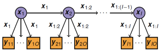
Figure 1.
Investment periods in circles and operational periods in boxes. The investment variables up to period l affect the next investment periods.
Generation and the power flow through transmission lines is constrained by capacity limits and ramping constraints. The DR module introduces new second-stage variables for the flexible load types, , as well as first-stage multi-period investment variables in DR technologies (i.e., endogenous expansion capacities). First-stage variables represent capacity expansion on generation, transmission, and storage. Second-stage variables represent operation of generators, interconnectors, and storages.
In the following we introduce the notation for flexible loads starting by the balance Equation (1). The module includes new DR operational variables called load deviation, for each flexible load , period , scenario and hour . It represents the up-regulation (positive) and down regulation (negative) of flexible loads. It also includes the load loss of activating flexible loads since we assume there exist DR rebound effects and operational inefficiencies, in the same way that storage and transmission have their own efficiencies , where is a storage unit and is an arc of the network. These efficiency factors are assumed to be constant in any grid operating state. We also assume ramp constraints, conventional generation, storage, and transmission limits to be constant.
The new second-stage variables are co-optimized with the network operational variables as generation , with a generator, storage , , transmission and lost load .
Stochasticity in the balance Equation (1) appears in the country load , flexible loads and through additional constraints (2) for the generation of variable renewable sources:
where is stochastic for wind, solar, and hydro power, and scenario independent for the rest of technologies, while , is a first-stage variable representing capacity of generator g. Constraints (2) link first and second-stage decisions.
The country load is assumed to include a share of inflexible loads and a share of flexible loads. To disaggregate the flexible share into each of the DR group loads, Equation (3) links country load, investment and operational variables in the same way that (2) links power supply operation and capacity. The available DR capacity depends on both the installed DR capacity, the actual time period and on the level of the stochastic country load. Variables are called potential load and are the available hourly load that potentially can be used by flexible load group f in hour h.
This capacity is calculated using two scaling factors. First, the deterministic constants take values in and represent the share of flexible load in each DR group in a given hour h considering weekday, weekend, and seasonal patterns. They capture the hourly availability factor for flexibility of each DR group. The second scaling factor is stochastic and depends on the scenario . For each node n, long-term period i and hour h it is based on the ratio between the actual load, , and the yearly peak load for the same long-term period. Those two scaling factors are multiplied with the installed DR capacity, , to find the DR potential in each hour and scenario.
To track the amount of shifted and curtailed loads for each class, an auxiliary variable, , called resulting load is defined in (4). It is a load (i.e., positive values) representing the actual country aggregated load value of flexible group f.
By definition, the resulting load in hour h is zero when . The load is unregulated when , upward regulated when and downward regulated when (the regulation range for the load deviation is not necessarily symmetric with respect to zero. An upper bound is defined for later (Appendix B), which in consequence bounds the load deviation).
The DR energy loss is the extra energy needed to shift or curtail load. The DR efficiency of load f, , is defined as the ratio between the load deviation and load deviation plus the energy loss. It follows from this definition that the energy loss is
where we model the energy loss assuming it equally distributed between the hours with load shift regulation. This sets the value 0.5 for shiftable loads to avoid double counting, that is
The deviations from the potential load are performed under a supply cost function, included in the objective function.
The following additional constraint is required to limit the up-regulation of a flexible load
The bounds are used to allow extra upward regulation during off-peak hours proportionally higher than in peak hours (asymmetric regulation). In other words, it allows load valley filling and restricts upward regulation precisely in peak hours. The upper bounds are year, scenario and flexible group specific and mathematically defined in Appendix C.
3.2.1. Shiftable Volume Load
A shiftable volume load in a time window , indexed by , can be replaced by a new load provided that their total energy is equal. In other words, the new energy consumption is the same as the original. This is represented as constraint (10) named DR-balance [41]. A shiftable volume load satisfies Equations (3)–(11). For each hour h the demand variables representing the shifted load, can have a larger or lower value than the original . The time window sub-intervals define the time span during which the load can be shifted and their size is limited by the maximum load-specific time shift parameter , . They must be intervals forming a partition of interval .
3.2.2. Curtailable Load
Curtailable loads can be adjusted from zero to the original value in a predefined time window , which means that they have to satisfy Equations (3)–(9) and the constraints (12)–(14).
Please note that shiftable resulting loads are allowed to be higher than the potential load, but curtailable loads are constrained by the potential load in (12). Because both shiftable resulting load and curtailable resulting loads are required to be non-negative, the downward regulation can be as low as .
3.2.3. Interruptible Load
3.3. DR Capacity
In the first-stage problem, DR investments and capacities are bounded. The upper bound capacity is set exogenously. The maximum investment in DR capacity in year i for load is denoted by . The relation between aggregated available capacity of load f in period i and investments depends on the operational life of the investment .
3.4. The New Objective Function
The operation of flexible loads is executed at a fixed a priori cost. If a flexible load diverges at a given hour from the value of the original load, then that change is penalized by a cost (8). Therefore, the load deviation is penalized either if it is positive or negative. In this model the costs are given by a convex piece-wise linear symmetric function, parametrized as follows. Abscissae are parametrized by variables , that form a Special Ordered Set (SOS2) through constants as shown in Equations (21)–(23), which are defined to be symmetric around the origin. Since the cost function is built to be convex there is no need to enforce the constraint that two consecutive to be non-zero. Ordinates , i.e., marginal costs, which are symmetric for load increase and decrease, are increased proportionally by the ratio on each piece (see Figure 2). More specifically, the first interval has costs of operation given by input data, denoted by in the cost function. The following intervals have increased marginal costs by the factor (24). In this way it is more and more costly to produce a change in the load profile (Please note that curtailable loads, since they can only be decreased, do not need variables on the positive axis, or equivalently, ).
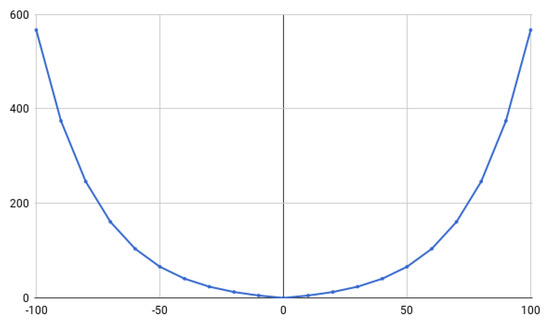
Figure 2.
Piece-Wise Linear Cost Function. The abscissa represent the percentage of upward and downward capacity and the ordinates represent the percentage cost of deviation.
The objective function is extended with two new terms: the investments in DR capacity and the cost of operation of flexible loads. The marginal costs are calculated through Equations (24)–(27). The investment cost per unit of power for group f is denoted by . The rest of the investment costs are denoted by where the index e is an index of the set of generators, arcs or storages (both for power storage and energy storage). The short run marginal cost of generator g in period i is represented by . The parameter u is the number of years between each investment period i (usually 5 years)
and = is a recovery factor to count the present value of each year within the investment period.
4. Demand Response Baseline Case
This section presents a study of the European power system and demonstrate the effects of DR. First follows an overview of the data used.
4.1. Demand Response Data
The DR potential upper bound, , comes from the estimated DR capacity in Gils [31]. This is also the main source for the values of the other parameters used in the DR module. In addition, Gils [50] provides hourly and seasonal variations for DR loads, and Gils [33] contains both investment and operation prices for each DR technology. Initial DR potentials come from Baker [29] where current European flexible potentials are assessed. Here the countries with highest DR potential are Belgium, Germany, Spain, France, Great Britain, Ireland, The Netherlands, Poland, Slovenia, and Sweden (This potential is measured by the ratio between the DR installed capacity and the country’s peak demand).
The DR technologies that represent flexible demand in the model are aggregated in the following 7 groups (see also Table A1): Heating and air conditioning (AC) in all sectors are flexible since they can be controlled according to the network and weather conditions. Heating Ventilation and AC (HVAC) are specific of large industries and commercial centers. Cooling and water includes all industrial and commercial appliances aimed to manage large food cooling systems or water supply systems. The process shift group includes the industrial processes pulp, paper, recycling paper, and cement. All of them allow a shift production hourly. Washing appliances comprises household appliances. Heat storage consists of appliances and installations that allow thermal storage. Finally, process shedding are industrial processes that can be partially stopped: aluminum, copper, zinc, chlorine and steel [31] (Table A2 shows the 2050 potentials).
The DR investment costs range from 0 to 250 k€/MW. The heating and air conditioning group has the highest investment cost because it requires installing remotely controlled equipment. Industrial DR investment costs are non-existent because DR is an inherent feature of industry operation, at different degrees according to each industrial sector. On average the DR investment costs are 45 k€/MW. The lower investment costs plus fixed O&M costs on DR technologies makes them competitive against lowest-cost generators (OCGT) and storage. However, variable O&M costs and capacity availability have also an impact on the optimal solution. The rest of generation technologies costs can be found in [49,51]. The group with the largest load-shifting time is the industrial shifting with 24 h, characteristic of a medium-term planning process, followed by heat storage with 12 h.
All the DR groups are shiftable volume loads, except for industrial process shedding which is a curtailable load type. Interruptible loads are not represented, as the problem size in the European model would make it intractable with flexible loads that require binary variables. The transport sector could not be included in the study case as load profiles for charging EVs were not available. The total energy demand by EVs is included in the study through the yearly demand input data. The electricity demand trends are based on the European commission 2016 reference case [1]. DR costs are homogeneous across countries and investment periods. The DR groups characteristics are presented in Table A1.
4.2. Short-Term Dynamics
Country load series are obtained from [52,53]. Wind and solar series are provided by the Renewables Ninja dataset [54,55,56], based on reanalysis data MERRA-2 by NASA [57] (Both data from load and IRES have been prepossessed to correct data measure errors and synchronize historical data in the period from 2010 to 2016).
The scenario generation routine based on moment matching creates the scenario tree representing the short-term uncertainty by sampling from a 7 year database consisting of hourly onshore wind, offshore wind, solar, and load data (The hydropower series are based on a synthetic approach that takes into consideration the countries maximum production [49]). It is based on [21] and finds a scenario tree that matches the mean, variance, skewness, and kurtosis of the historical data. Each scenario consists of 4 seasons with 168 consecutive hours each for load, wind, solar, and hydro, sampled from the same point in time across all countries. In addition, there are 24 extra hours for two extreme operating conditions: (a) Day with single highest peak net load and (b) Day with lowest global IRES energy generation. That makes 672 h per scenario, in 10 scenarios per short-term period over 9 long-term periods, making up 60,480 representative hours in total for the model horizon. The simulations performed with these input data are stable with respect to the scenario trees.
To represent the operational conditions of several years using representative hours, the first step is to cluster the data into four seasons. Within each season, a sample is a segment of d consecutive days with 24 h each. In the underlying data for a year, a season of 3 months has exactly 91 days or 2186 h. This gives groups of d days. If Y is the number of years in the sample space, then in total groups configure that season’s sample space. Each short-term scenario has 4 seasons (linked to an investment period) represented by 4 sampled seasons with d consecutive days, thereby keeping the chronological order for all in each season. A set of S scenarios makes a scenario tree. The scenario trees that best approximate the statistical properties of the random variables are used as input data. The scenario trees are sampled independently. This approach guarantees that the autocorrelation and cross-correlations of the population time series is kept for the representative days within a season.
4.3. Baseline Case Analysis
In the baseline case the upper bound for the DR is set exactly at the DR potential of each DR group in each country (Table A2).
There are considerable DR capacity increases in most countries during the investment period (Figure 3). The DR-to-peak ratio (DR capacity divided by peak demand) and the DR to IRES ratio (DR capacity divided by total IRES generation capacity) give insight on the DR uptake. In the final period (2050) the total DR-to-peak ratio amounts to 34.5% of European winter season peak demand, while the initial DR-to-peak ratio is 0.8%. Still, there are variations between countries, as shown in Table 1, with the lowest ratio in the United Kingdom (5.4%) and the highest in Hungary (40.8%). When it comes to the global DR to IRES ratio, the variation goes from 0.4% to 5.8% during the optimization horizon. The top 10 countries show a moderate DR to IRES ratio ranging from 4.8% to 11.7%. The top-10 countries have a 6.9% DR to IRES ratio and accumulate 81% of European installed flexible loads.
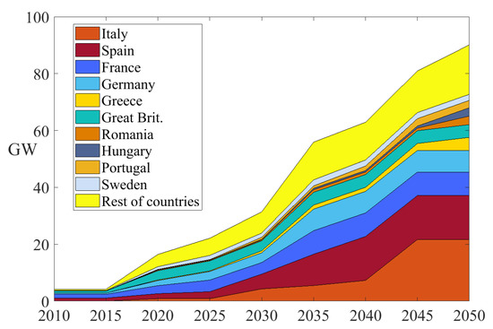
Figure 3.
Total DR Capacity Evolution from 2010 to 2050 of top DR countries in GW.

Table 1.
10 highest DR capacities in 2050 and initial DR capacity in 2015 together with other ratios.
4.3.1. DR Operation
The first DR impact is on the hourly load profile. In all countries and all long-term periods, the results show that there is load upward regulation when the inter-hour price difference is higher than the cost of flexible load arbitrage. The net load profile is defined as load minus IRES production (Figure 4). When the IRES production varies it creates peaks and valleys in the net load. The valleys, are used for upward regulation and there is downward regulation during the peaks. The effect is especially stressed in countries with high solar capacity such as Spain (Figure 4). A 48 h load sample shows DR events like peak shavings in the order of 10 GW in Spain and 3 GW in France in the load profile during winter. DR regulation events depend strongly on the daily solar peak production creating substantial electricity price differentials, as opposed to wind power which is more stable throughout. Another factor influencing DR is the power mix of each specific country. Systems dominated by dispatchable power plants have less price volatility.
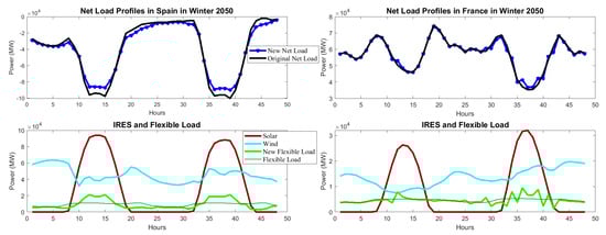
Figure 4.
Sample load profiles in Spain and France in 2050. Net load refers to total load minus IRES production, the term ‘new’ to the profile with active DR, ‘new flexible load’ is the resulting load of all flexible groups and ‘flexible load’ is their potential load.
4.3.2. Analysis of DR and System Capacities
In 2050, the global DR activity amounts to 95.8 TWh, which is 2.4% of the yearly net generation and 22% of total available flexible energy. Across the long-term planning horizon a total of 295 TWh have been changed by DR loads, while 1274 TWh keeps the original load pattern. In this part the system’s installed capacity and energy mix are analysed (Figure 5).
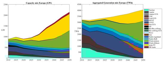
Figure 5.
Europe’s DR and Generation Capacity (GW) and Energy Generation (TWh).
The major investment in DR capacity occurs in the sixth period (27 GW). The DR groups in descending order of capacity are (6) heat storage (41 GW), (2) HVAC (23 GW), (4) process shift (10 GW), (7) process shedding (8 GW), (3) cooling and water (8 GW), (5) washing appliances (1 GW) and (1) heating and AC with (0.3 GW). The reasons that groups 2, 4 and 6 have the largest capacities are diverse: (a) heat storage has the 2nd largest shifting time Table A1, (b) HVAC has the lowest variable cost and (c) industry process shift has the largest time window even though its variable cost is the second largest (Since the investment cost of groups industry process shift and process shedding are zero their capacity is adjusted a posteriori to their actual maximum operational values in each country). The three largest total investments are led by the same groups heat storage, HVAC and process shift with 38 GW, 22 GW, and 10 GW, respectively. There are no investments in groups heating and AC, and washing appliances. The former has high investment cost. The latter has cost characteristics disadvantageous in comparison to HVAC (Table A1). Investments in groups cooling and shedding represent only 18% of all DR investments, leaving the main share, 82%, for groups 2, 4 and 6. For country average, the capacity of groups 2 and 3 reaches full potential in period 4, while the groups 1, 5 and 6 do not reach the capacity’s upper theoretical potential at the end of the horizon.
In the final period, 7 out of 10 countries with high installed IRES (onshore wind, offshore wind and solar) are among the 10 highest regarding DR installed capacities. The 10 countries with the highest DR capacity in 2050 have a total of 80% of European DR capacity, 67% of IRES installed capacity and 68% of total installed capacity.
The renewable that receives the most investments globally is solar, with an accumulated increase from 2010 to 2050 of 748 GW, followed by onshore wind with 718 GW. The main solar investment happens in 2035 with 234 GW. This corresponds to an annual increase rate of 17% with respect to solar capacity in 2030. Considering all the renewable technologies, there are 9 countries with more than 90% IRES share in 2050 (of which only Spain and Hungary are also in the previous top-10). Europe’s IRES share amounts to 76%.
Regarding technologies that can compete with DR by providing generation flexibility to the system, ramping capacity, and peak supply, it is interesting to see the changes in the following gas technologies. Existing stock gas turbines, Open Cycle Gas Turbines (OCGT), Closed Cycled Gas Turbines (CCGT) and gas with Carbon Capture and Storage (CCS), whose high ramping rates, can supply power during residual demand peak periods. This group of gas turbines has an increase of 35% caused mainly by gas CCGT power and investments in CCS from 2040. At that point, backup capacity from CCS substitutes the already abated nuclear power.
In a second group, regulated hydro power, hydro pump storage, and battery storage can store energy for periods with scarcity of supply. Their installed power capacity has a slight increase of 21% between 2010 and 2050. Regulated hydro power and hydro pumped storage have moderate increases at around 16%. Battery storage becomes cost-effective exactly when the solar capacity starts the large investments by 2030–2040.
Transmission capacity sums up to 501 GW by 2050, with the major investments happening when solar capacity reaches system dominance. This represents a significant increase of 700% interconnector capacity. The most reinforced transmission corridors are Spain–France, France–Great Britain, Poland–Germany, Poland–Lithuania, Poland–Czech Republic and Italy–France with total capacities in 2050 of 83 GW, 52 GW, 30 GW, 13 GW, 13 GW, and 12 GW respectively. The countries with highest aggregated transmission capacity in 2050 are France (179 GW), Germany (104 GW) and Spain (89 GW).
The emission constraints imposing a linearly decreasing emission cap from 2010 to 2050 (90% reduction with respect to 2010s emissions in EU aggregated) is binding in all periods. The carbon price (Given as the shadow price of the emission constraint) decreases from 41 €/EUA in 2020 to 32 €/EUA in 2030. From that point carbon price increases steadily to 86 €/EUA in 2050. In the results, there are many countries that decrease their emissions by 100% in 2050: Norway, Sweden, Finland and Austria (although they might be dependent on imports). In total there are 14 countries with reductions of more than 98%.
Average electricity cost increases from 42.0 €/MWh by 2020 to 53.2 €/MWh by 2050. The increase is caused mainly by increased investment costs, despite that non-polluting technologies have decreasing costs. Part of the increase is caused by high costs of CCS technologies, which are necessary to cover the demand. Investments in CCS start in year 2035 with 4 GW total installed, then a 10-fold increase in 2040, reaching at the final period a capacity of 85 GW in total.
The results above do not consider the use of DR in ancillary services or for local flexibility markets. This would most likely require a finer time resolution and geographical resolution in the model. In moments with limited DR capacity, part of it would be reserved for other uses than the ones represented in EMPIRE. The value of flexibility may be even higher in those applications.
4.4. No DR Case
The model outcomes with disabled DR investments and operation are compared to the baseline case, and the four main differences can be seen in Table 2. The difference in IRES installed capacity is caused by a higher solar capacity in the baseline (DRB) than in the no DR case (DR0), which is a consequence of the availability of shifting load to high solar production periods. Flexible loads allow taking advantage from solar production, which has 75% lower investment cost than onshore wind. This leads to the second main difference: a 7.8% higher curtailment of IRES in DRB than in DR0, which is explained by the fact that in certain days the solar production is high but not enough to make a significant price difference that can be economically efficient for more load-shifting. That electricity surplus that alternatively could be used in other sectors is not included in the model.
Table 2.
Main differences between cases DR0 and DRB in 2050.
Despite the curtailment difference in 2050, the IRES annual generation is approximately the same until 2035, where DRB shows more production from IRES and less from peak plants (by 2050 in DRB there is only 1.8% more production). If we look into wind and solar separately, DRB has more generation of both from 2030 to 2050 except only for 2040 (when a high investment in solar capacity causes a change in the sign of production).
The third difference is that flexible loads allow significant savings on peak plants in DRB because the net demand peaks are reduced. Finally, the fourth difference appears in power storage capacity, with 86% more capacity in DR0 than in DRB. The battery energy capacity is 18 times higher in DR0. In this case, it is clear that the availability of flexible loads reduces the needs of investments in storage infrastructure. However, the DR loads cannot substitute all the storage power and energy capacity needed.
When it comes to generation from the peak power plants, there are low differences in 2020 and 2025 when solar still has low shares in the energy mix (Figure 6). In 2035 the electricity generated from peak plants is higher in DR0 than in DRB. From next period a trend switch starts: in DRB there is more generation from CCGT and less from CCS than in DR0. Therefore, only in peak plants, the DRB’s energy mix has higher emission intensity (which is compensated by a major IRES electricity production). The main 2050 generation differences comes from CCS, onshore wind and solar with −68 TWh, +17 TWh and +32 TWh, respectively.
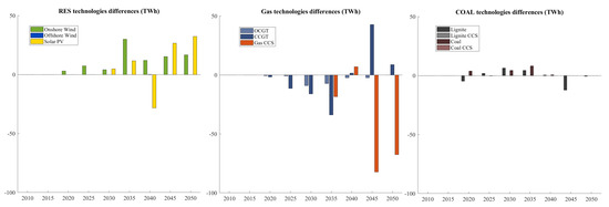
Figure 6.
Europe’s Generation Difference between DR0 and DRB by period. Positive y-axis indicates larger energy generation in DRB than in DR0 and vice versa.
The overall average electricity price without DR technologies follows the same evolution as in DRB but are 2% higher from 2035 due to a lower IRES integration and the need for gas CCS. The CCS capacities in DR0 are two times higher than 2035 DRB ones, and decrease until 2050 when they set at 16%.
The differences in energy generation reflect the differences on capacity portfolio (and vice versa). Total generation investments are in fact very similar in both cases (2059 GW). Aggregating storage power and transmission capacity to the mix results in DR0 requiring in fact 50 GW more than DRB. These 50 GW are compensated in DRB by the virtual infrastructure (or ICT capacity) of flexible consumers, with 91 GW.
It is interesting to analyse the capacity mix in 2035 because by then there is a huge 25 GW DR investment, solar PV rise and current fossil fuel plants are about to be decommissioned. In DRB there is more onshore wind and solar capacity, while in DR0 there are more peak plants (Figure 7). That is the moment when both cases start to diverge. From 2045 to 2050, DRB’s capacity portfolio is based on solar and DR flexible loads, while the DR0 case has to make use of gas CCS, onshore wind, and solar production through storage (The portfolio of lignite and coal plants is the same in both cases until 2050 with minor differences in generation).
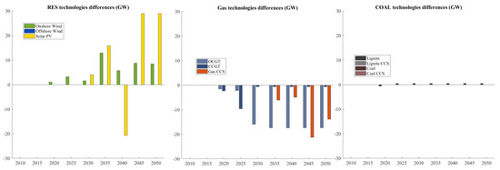
Figure 7.
Europe’s Capacity Difference between DR0 and DRB by year. Positive y-axis indicates larger capacity in DRB than in DR0 and the negative side less capacity.
4.5. Sensitivity Analysis
4.5.1. Capacity Sensitivity
A sensitivity analysis is performed on the total DR capacity of each country. The upper limit is specified relative to the theoretical DR potential in DRB by using the following scaling factors: 0.5, 0.75, 1.25 and 1.5 compared to the DR capacity in DRB (Table A2), for cases DR1 to DR4, respectively. In the model this is implemented through constraints (19).
Table 3 shows the percentage variation with respect to the reference case DRB. We see that relaxing the DR total capacity constraint (DR3 and DR4) allows more DR capacity into the system, more solar PV, more IRES curtailment, less peak plant capacity globally and less gas CCS. The sequence of cases shows around 20% change in DR capacity while solar capacity changes by 1% and storage power capacity by 2–6%.
Table 3.
Relative differences of each sensitivity case in percentage with respect to the reference case DRB (%).
The groups with highest DR capacity in all the cases are groups 6 (heat storage), 2 (HVAC) and 5 (washing appliances), except in DR4 where group 3 takes group 5’s third position. In particular, in DR4 their capacities are 234 GW, 30 GW, and 11.7 GW respectively, which added to the rest of the group totals 315 GW.
4.5.2. Costs Sensitivity
To analyse how costs affect the uptake of DR capacity, sensitivity cases DRC1-DRC5 scales both the investment and operational costs of all the DR groups with the following factors: 0.25, 0.5, 2, 4, and 8. In Table 4 the main differences between cases are represented in percentage. As expected the amount of DR capacity decreases with increasing costs. There is less IRES, solar capacity and generation when less DR capacity is available. IRES curtailment is higher in DRC1 and DRC2 than in DRB because they have higher solar capacity. High costs of DR make solar capacity less efficient as can be observed in cases DRC3 to DRC5. The reason is that operational costs in DRC1 and DRC2 make it efficient to shift more energy to the IRES production hours. In DRC4 and DRC5 the curtailment is lower than in DRB since there is less IRES hourly surplus during the normal and low demand seasons. Storage capacity differences are significant (−9% to 38% in DRC1–DRC5), with storage and DR capacity as substitute technologies. High differences in storage capacity arise in 2035 and onwards in cases DRC3–DRC5 in comparison to DRB (Figure 8).
Table 4.
DR costs sensitivity’s percentage variation analysis respect to DRB (%).
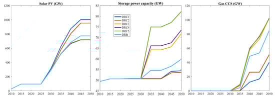
Figure 8.
Europe’s Capacity Development by year between DRB and DRC1-5 cases.
Although total installed capacity decreases with increasing DR costs (due to solar capacity), the capacity of peak plants (+11%) and in particular gas CCS (+20%) increase. Electricity prices are down to -8% cheaper in DRC1 and stay stable at +3% in DRC3 to DRC5.
5. Conclusions
This paper describes how to implement a DR module in a capacity expansion model for the European power markets. The case study includes endogenous DR investments co-optimized with intermittent renewable sources, other generation technologies, storage, and transmission. Flexible demand is aggregated in groups of end consumers that share similar characteristics, investment, and operative costs. Two types of flexible loads have been used in the case study, shiftable volume loads and curtailable loads. These two types of DR can be modelled with linear variables, whereas interruptible loads require binary variables.
DR’s development in Europe has been assessed for seven different end-consumer groups. The results show that the main contributor to load-shifting measured by energy volume is heat storage end uses, followed by industrial process shifting. These are the groups that offer the most flexible timeframes for DR. Investments in DR capacities happen because flexible loads provide a more efficient way to handle intermittent solar energy than alternatives. We see that the countries with the highest IRES capacities also have the highest DR investments. The model applies load-shifting during periods of high solar production and residual load sudden variations.
The adoption of demand-responsive loads has impacts on the power system. Particularly relevant is the fact that gas power plants supplying flexible energy during peak events are partially substituted by the flexibility offered by DR loads. On one hand, DR introduces more degrees of freedom into the model. It allows more IRES integration into the system and fewer capital investments in peak plants. On the other hand, investments in polluting plants are affordable in gas OCGT with low investment costs. In that sense, DR alone is not a technology that would allow a significant reduction of emissions.
Solar PV and onshore wind capacities follow similar paths because the former is more efficient in southern countries while the latter is efficient in the Nordic ones and the British Islands. By 2050 their installed capacities will be 774 GW and 802 GW, respectively. Countries with the highest installed DR capacities are the ones with the highest solar capacity.
The impacts to the power system are not extreme in the sense of turning around the capacity mix. DR capacities act as a support technology by integrating 2% more IRES, saving 11% of peak capacity and 86% of storage capacity, and therefore facilitating the transition towards a system with high shares of renewable sources.
Author Contributions
Conceptualization, H.M.-L. and A.T.; methodology, H.M.-L.; software, H.M.-L.; validation, H.M.-L.; formal analysis, H.M.-L.; investigation, H.M.-L.; resources, H.M.-L. and A.T.; data curation, H.M.-L.; writing–original draft preparation, H.M.-L.; writing–review and editing, H.M.-L. and A.T.; visualization, H.M.-L.; supervision, H.M.-L. and A.T.; project administration, H.M.-L.; funding acquisition, A.T.
Funding
The research of this paper has been conducted in the Center for Sustainable Energy Studies (CenSES) from The Research Council of Norway with project number 209697. The author thanks the support from the European Union’s Horizon 2020 project “SET-Nav” (No. 691843).
Conflicts of Interest
The authors declare no conflict of interest. The funders gave approval to publish the results.
Appendix A. DR Input Data
Table A1.
DR technology costs for the 7 groups considered in the model and other technology costs for comparison. Sectors: 1. Residential, 2. Industrial, 3. Commercial, DR source: Gils [33].
Table A1.
DR technology costs for the 7 groups considered in the model and other technology costs for comparison. Sectors: 1. Residential, 2. Industrial, 3. Commercial, DR source: Gils [33].
| Technology | Sector | Investment Cost (k€/MW) | Fixed OM (€/MW) pr. yr. | Variable OM (€/MWh) | Efficiency | Max. Time Shift (h) |
|---|---|---|---|---|---|---|
| 1. Heating & AC | All | 250 | 7500 | 10 | 0.97 | 2 |
| 2. HVAC | 2, 3 | 10 | 300 | 5 | 0.97 | 2 |
| 3. Cooling & Water | 2, 3 | 5 | 150 | 20 | 0.98 | 6 |
| 4. Process Shift | 2 | 0 | 0 | 150 | 0.99 | 24 |
| 5. Washing appliances | 1 | 30 | 900 | 50 | 1.00 | 6 |
| 6. Heat Storage | 1, 3 | 20 | 600 | 10 | 0.98 | 12 |
| 7. Process Shedding | 2 | 0 | 0 | 1000 | 1.00 | - |
| Gas OCGT | 400 | 1950 | 0,45 | - | ||
| Battery Storage (Zn) | 588 | 0.75 | ||||
| Battery Storage (Li-ion) | 400 | 0.88 | ||||
| Pumped-Storage Hydro | 1000 | 0.80 |
Table A2.
DR potentials in GW. Adapted from Gils [33].
Table A2.
DR potentials in GW. Adapted from Gils [33].
| Country | Class 1 | Class 2 | Class 3 | Class 4 | Class 5 | Class 6 | Class 7 | Total |
|---|---|---|---|---|---|---|---|---|
| Europe | 23.2 | 22.7 | 7.8 | 9.5 | 63.4 | 156.1 | 8.8 | 291.5 |
| France | 3.0 | 3.6 | 1.3 | 1.6 | 8.1 | 26.0 | 0.8 | 44.3 |
| Germany | 4.2 | 3.1 | 1.1 | 1.4 | 13.1 | 17.8 | 1.7 | 42.5 |
| Great Brit. | 2.7 | 2.3 | 0.8 | 0.5 | 9.1 | 21.5 | 0.3 | 37.1 |
| Italy | 2.7 | 2.6 | 0.8 | 0.9 | 6.8 | 16.2 | 1.3 | 31.4 |
| Spain | 2.2 | 2.8 | 0.8 | 0.8 | 4.1 | 9.6 | 1.2 | 21.5 |
| Poland | 1.2 | 1.0 | 0.4 | 0.3 | 2.8 | 8.5 | 0.3 | 14.5 |
| Sweden | 0.5 | 0.8 | 0.3 | 0.8 | 1.6 | 8.7 | 0.2 | 12.8 |
| Norway | 0.2 | 0.7 | 0.2 | 0.3 | 0.8 | 6.8 | 0.5 | 9.6 |
| The Netherlands | 0.7 | 0.8 | 0.3 | 0.2 | 3.0 | 3.6 | 0.1 | 8.8 |
| Finland | 0.2 | 0.4 | 0.2 | 1.0 | 0.8 | 5.4 | 0.2 | 8.1 |
| Romania | 0.6 | 0.2 | 0.1 | 0.2 | 1.1 | 4.0 | 0.4 | 6.5 |
| Belgium | 0.5 | 0.5 | 0.2 | 0.2 | 1.7 | 2.8 | 0.3 | 6.3 |
| Greece | 0.6 | 0.6 | 0.2 | 0.2 | 0.9 | 3.2 | 0.5 | 6.2 |
| Austria | 0.4 | 0.3 | 0.1 | 0.2 | 1.3 | 2.5 | 0.1 | 4.9 |
| Czech R | 0.4 | 0.3 | 0.1 | 0.1 | 0.9 | 2.5 | 0.1 | 4.4 |
| Switzerland | 0.4 | 0.4 | 0.1 | 0.1 | 1.2 | 2.0 | 0.1 | 4.2 |
| Hungary | 0.4 | 0.3 | 0.1 | 0.1 | 0.7 | 2.4 | 0.1 | 4.1 |
| Portugal | 0.4 | 0.4 | 0.1 | 0.2 | 1.1 | 1.8 | 0.1 | 4.1 |
| Denmark | 0.3 | 0.2 | 0.1 | 0.1 | 1.1 | 1.6 | 0.0 | 3.4 |
| Slovakia | 0.2 | 0.2 | 0.1 | 0.1 | 0.5 | 1.6 | 0.1 | 2.7 |
| Bulgaria | 0.3 | 0.2 | 0.1 | 0.1 | 0.4 | 1.4 | 0.1 | 2.5 |
| Ireland | 0.2 | 0.2 | 0.1 | 0.1 | 0.6 | 1.3 | 0.0 | 2.4 |
| Serbia | 0.2 | 0.1 | 0.0 | 0.1 | 0.4 | 1.1 | 0.0 | 2.0 |
| Croatia | 0.2 | 0.1 | 0.0 | 0.1 | 0.3 | 0.6 | 0.0 | 1.4 |
| Lithuania | 0.1 | 0.1 | 0.0 | 0.0 | 0.3 | 0.8 | 0.0 | 1.3 |
| Slovenia | 0.1 | 0.1 | 0.0 | 0.0 | 0.3 | 0.6 | 0.1 | 1.1 |
| Latvia | 0.1 | 0.1 | 0.0 | 0.0 | 0.1 | 0.7 | 0.0 | 0.9 |
| Bosnia H | 0.1 | 0.0 | 0.0 | 0.0 | 0.1 | 0.5 | 0.1 | 0.8 |
| Estonia | 0.1 | 0.1 | 0.0 | 0.0 | 0.1 | 0.4 | 0.0 | 0.7 |
| Luxemb. | 0.0 | 0.0 | 0.0 | 0.0 | 0.1 | 0.1 | 0.2 | 0.5 |
| Macedonia | 0.0 | 0.0 | 0.0 | 0.0 | 0.1 | 0.3 | 0.0 | 0.5 |
Appendix B. Other Types of Flexible Loads
Appendix B.1. Shiftable Profile Load
Shiftable profile loads constraints can be represented through time shift variables . They satisfy Equations (3)–(9) and (A1)–(A3) (We use a non-standard notation placing the variable as an index of another variable ). For a possible implementation of this load with integer variables the reader is referred to [41].
Appendix B.2. Flexible-Curtailment Load
A fifth type of load is a flexible load that can be either curtailed or increased with no cost and no DR balance (Equation 10). That kind of load could be an industry that increases production in times of negative electricity prices or when oversupply could destabilize the power system. This is a flexible load which fulfils constraints (3)–(9), (A4) and (A5) and its costs are zero for load increase.
Appendix C. Upper Bound Mathematical Definition
The objective of the upper bounds is to limit load-shifting and allow sufficient valley filling.
Given a load and a constant , the scaled load is the component-wise scaling .
The load ramps are defined as the consecutive hour differences of the scaled load
Ramp selection consists of defining the positive and negative ramps as follows.
The ramps and contain the absolute values of the positive and negative ramps separately. Their objective is to add a variable slack to the potential flexible load in each hour h that depends on the neighbour values to h of that load.
Given an hour h, the load is: (a) a local minimum if the corresponding ramps and are positive (equivalently ), (b) a local maximum if the ramps (equivalently ), (c) in descending slope if and and (d) ascending slope if and . The principle to add up neighbouring ramps in a given hour is basically to add up all upcoming positive ramps and all previous negative ramps. In this way a local minimum load accumulates all the neighbouring ramps and proportionally takes more slack increase than the peaks.
The ramp time window parameters and select the neighbouring ramps that define the upper bound. selects the ramps after hour h (to the right) and selects the ramps before hour h (to the left). Extra parameters taking values in are used as weights to scale the values of the ramps. The parameters’ values A, and can be based on assumptions or adjusted with an empirical method. The mathematical formula for the upper bound is as follows.
According to the definition if is a local maximum in , then the corresponding ramps are 0 (Unless there are consecutive local minimum and maximum within ), the two summations in the definition are zero and the upper bound is just the first term .
The upper bound depends on the choice of the constants . Because the input data for each load group specifies that each hour load is the potential for both upward regulation and downward regulation, it is logical to choose . That means each resulting load has an available range to increase of at least , regardless of the other parameters. According to the flexible load profiles, their variations happen in a time window of 6 h. Because of using uniform parameters in this study the values chosen are h (6 ramps in total) and for all flexible loads f, periods i and hours h and t.
References
- Capros, P.P.; Vita, A.D.; Tasios, N.; Siskos, P.; Kannavou, M.; Petropoulos, A.; Evangelo-Poulou, S.; Zampara, M.; Papadopoulos, D.; Paroussos, L.; et al. EU Reference Scenario 2016—Energy, Transport and GHG Emissions Trends to 2050; Technical Report; European Commission Directorate-General for Energy, Directorate-General for Climate Action and Directorate-General for Mobility and Transport; Publications Office of the European Union: Luxembourg, 2016. [Google Scholar]
- Albadi, M.H.; El-Saadany, E.F. A summary of demand response in electricity markets. Electr. Power Syst. Res. 2008, 78, 1989–1996. [Google Scholar] [CrossRef]
- Jägemann, C.; Fürsch, M.; Hagspiel, S.; Nagl, S. Decarbonizing Europe’s power sector by 2050—Analyzing the economic implications of alternative decarbonization pathways. Energy Econ. 2013, 40, 622–636. [Google Scholar] [CrossRef]
- Göransson, L.; Goop, J.; Unger, T.; Odenberger, M.; Johnsson, F. Linkages between demand-side management and congestion in the European electricity transmission system. Energy 2014, 69, 860–872. [Google Scholar] [CrossRef]
- Zerrahn, A.; Schill, W.P. On the representation of demand-side management in power system models. Energy 2015, 84, 840–845. [Google Scholar] [CrossRef]
- Skar, C.; Doorman, G.; Tomasgard, A. The future European power system under a climate policy regime. In Proceedings of the Energy Conference (ENERGYCON), Dubrovnik, Croatia, 13–16 May 2014; IEEE International: Piscataway, NJ, USA, 2014; pp. 318–325. [Google Scholar] [CrossRef]
- Ulbig, A.; Andersson, G. Analyzing operational flexibility of electric power systems. (The Special Issue for 18th Power Systems Computation Conference). Int. J. Electr. Power Energy Syst. 2015, 72, 155–164. [Google Scholar] [CrossRef]
- Bastida, L.; Cohen, J.J.; Kollmann, A.; Moya, A.; Reichl, J. Exploring the role of ICT on household behavioural energy efficiency to mitigate global warming. Renew. Sustain. Energy Rev. 2019, 103, 455–462. [Google Scholar] [CrossRef]
- Lund, P.D.; Lindgren, J.; Mikkola, J.; Salpakari, J. Review of energy system flexibility measures to enable high levels of variable renewable electricity. Renew. Sustain. Energy Rev. 2015, 45, 785–807. [Google Scholar] [CrossRef]
- Mathieu, J.L.; Kamgarpour, M.; Lygeros, J.; Andersson, G.; Callaway, D.S. Arbitraging intraday wholesale energy market prices with aggregations of thermostatic loads. IEEE Trans. Power Syst. 2015, 30, 763–772. [Google Scholar] [CrossRef]
- Ilić, M.D.; Popli, N.; Joo, J.Y.; Hou, Y. A possible engineering and economic framework for implementing demand side participation in frequency regulation at value. In Proceedings of the IEEE Power and Energy Society General Meeting, Detroit, MI, USA, 24–29 July 2011; IEEE: Piscataway, NJ, USA, 2011; pp. 1–7. [Google Scholar] [CrossRef]
- Blum, D.H.; Xu, N.; Norford, L.K. A novel multi-market optimization problem for commercial heating, ventilation, and air-conditioning systems providing ancillary services using multi-zone inverse comprehensive room transfer functions. Sci. Technol. Built Environ. 2016, 22, 783–797. [Google Scholar] [CrossRef]
- Kall, P.; Wallace, S.W. Stochastic Programming, 2nd ed.; John Wiley & Sons: Chichester, UK, 1994. [Google Scholar]
- Kaut, M.; Midthun, K.T.; Werner, A.S.; Tomasgard, A.; Hellemo, L.; Fodstad, M. Multi-horizon stochastic programming. Comput. Manag. Sci. 2013, 11, 179–193. [Google Scholar] [CrossRef]
- Poncelet, K.; Höschle, H.; Delarue, E.; Virag, A.; D’haeseleer, W. Selecting Representative Days for Capturing the Implications of Integrating Intermittent Renewables in Generation Expansion Planning Problems. IEEE Trans. Power Syst. 2017, 32, 1936–1948. [Google Scholar] [CrossRef]
- Pfenninger, S.; Hawkes, A.; Keirstead, J. Energy systems modeling for twenty-first century energy challenges. Renew. Sustain. Energy Rev. 2014, 33, 74–86. [Google Scholar] [CrossRef]
- Nahmmacher, P.; Schmid, E.; Hirth, L.; Knopf, B. Carpe diem: A novel approach to select representative days for long-term power system modeling. Energy 2016, 112, 430–442. [Google Scholar] [CrossRef]
- Seljom, P. Stochastic Modelling of Short-Term Uncertainty in Long-Term Energy Models: Applied to TIMES Models of Scandinavia. Ph.D. Thesis, Norwegian University of Science and Technology, Trondheim, Norway, 2017. [Google Scholar]
- Eurek, K.; Cole, W.; Bielen, D.; Blair, N.; Cohen, S.; Frew, B.; Ho, J.; Krishnan, V.; Mai, T.; Sigrin, B.; et al. Regional Energy Deployment System (Reeds) Model Documentation: Version 2016; Technical Report; National Renewable Energy Lab. (NREL): Golden, CO, USA, 2016. [Google Scholar]
- Nicolosi, M.; Mills, A.D.; Wiser, R.H. The Importance of High Temporal Resolution in Modeling Renewable Energy Penetration Scenarios; Technical Report; Lawrence Berkeley National Lab. (LBNL): Berkeley, CA, USA, 2010. [Google Scholar]
- Seljom, P.; Tomasgard, A. Short-term uncertainty in long-term energy system models—A case study of wind power in Denmark. Energy Econ. 2015, 49, 157–167. [Google Scholar] [CrossRef]
- Ringkjøb, H.K.; Haugan, P.M.; Solbrekke, I.M. A review of modelling tools for energy and electricity systems with large shares of variable renewables. Renew. Sustain. Energy Rev. 2018, 96, 440–459. [Google Scholar] [CrossRef]
- Helistö, N.; Kiviluoma, J.; Holttinen, H.; Lara, J.D.; Hodge, B.M. Including operational aspects in the planning of power systems with large amounts of variable generation: A review of modeling approaches. Wiley Interdiscip. Rev. Energy Environ. 2019, e341. [Google Scholar] [CrossRef]
- Fernández-Blanco Carramolino, R.; Careri, F.; Kavvadias, K.; Hidalgo-Gonzalez, I.; Zucker, A.; Peteves, E. Systematic Mapping of Power System Models—Expert Survey; Technical Report; European Commision—JRC Technical Reports; Publications Office of the European Union: Luxembourg, 2017. [Google Scholar]
- SEDC (Smart Energy Demand Coalition). Mapping Demand Response in Europe Today 2015; Technical Report; SEDC Smart Energy Demand Coalition: Brussels, Belgium, 2015. [Google Scholar]
- SEDC (Smart Energy Demand Coalition). Explicit Demand Response in Europe. Mapping the Markets 2017; Technical Report; SEDC Smart Energy Demand Coalition: Brussels, Belgium, 2017. [Google Scholar]
- Torriti, J.; Hassan, M.G.; Leach, M. Demand response experience in Europe: Policies, programmes and implementation. Energy 2010, 35, 1575–1583. [Google Scholar] [CrossRef]
- Müller, F.; Jansen, B. Large-scale demonstration of precise demand response provided by residential heat pumps. Appl. Energy 2019, 239, 836–845. [Google Scholar] [CrossRef]
- Baker, P. Resource Adequacy, Regionalisation and Demand Response; Technical Report; The Regulatory Assistance Project (RAP): Montpelier, VT, USA, 2015. [Google Scholar]
- ENTSO-e. Scenario Outlook and Adequacy Forecast 2015; Technical Report; ENTSO-e: Brussels, Belgium, 2015. [Google Scholar]
- Gils, H.C. Assessment of the theoretical demand response potential in Europe. Energy 2014, 67, 1–18. [Google Scholar] [CrossRef]
- Bossmann, T.; Eser, E.J. Model-based assessment of demand-response measures—A comprehensive literature review. Renew. Sustain. Energy Rev. 2016, 57, 1637–1656. [Google Scholar] [CrossRef]
- Gils, H.C. Economic potential for future demand response in Germany—Modeling approach and case study. Appl. Energy 2016, 162, 401–415. [Google Scholar] [CrossRef]
- Schill, W.P.; Zerrahn, A. Long-run power storage requirements for high shares of renewables: Results and sensitivities. Renew. Sustain. Energy Rev. 2018, 83, 156–171. [Google Scholar] [CrossRef]
- Kies, A.; Schyska, B.U.; Von Bremen, L. The Demand Side Management Potential to Balance a Highly Renewable European Power System. Energies 2016, 9, 955. [Google Scholar] [CrossRef]
- Zerrahn, A.; Schill, W.P. Long-run power storage requirements for high shares of renewables: Review and a new model. Renew. Sustain. Energy Rev. 2017, 79, 1518–1534. [Google Scholar] [CrossRef]
- Papadaskalopoulos, D.; Moreira, R.; Strbac, G.; Pudjianto, D.; Djapic, P.; Teng, F.; Papapetrou, M. Quantifying the Potential Economic Benefits of Flexible Industrial Demand in the European Power System. IEEE Trans. Ind. Inform. 2018, 14, 5123–5132. [Google Scholar] [CrossRef]
- Müller, T.; Möst, D. Demand Response Potential: Available when Needed? Energy Policy 2018, 115, 181–198. [Google Scholar] [CrossRef]
- De Jonghe, C.; Hobbs, B.F.; Belmans, R. Optimal Generation Mix with Short-Term Demand Response and Wind Penetration. IEEE Trans. Power Syst. 2012, 27, 830–839. [Google Scholar] [CrossRef]
- Lohmann, T.; Rebennack, S. Tailored Benders Decomposition for a Long-Term Power Expansion Model with Short-Term Demand Response. Manag. Sci. 2016. [Google Scholar] [CrossRef]
- Ottesen, S.; Tomasgard, A. A stochastic model for scheduling energy flexibility in buildings. Energy 2015, 88, 364–376. [Google Scholar] [CrossRef]
- García-Garre, A.; Gabaldón, A.; Álvarez-Bel, C.; Ruiz-Abellón, M.D.C.; Guillamón, A. Integration of Demand Response and Photovoltaic Resources in Residential Segments. Sustainability 2018, 10. [Google Scholar] [CrossRef]
- Ottesen, S.; Tomasgard, A.; Fleten, S.E. Prosumer bidding and scheduling in electricity markets. Energy 2016, 94, 828–843. [Google Scholar] [CrossRef]
- Sáez-Gallego, J.; Kohansal, M.; Sadeghi-Mobarakeh, A.; Morales, J.M. Optimal Price-Energy Demand Bids for Aggregate Price-Responsive Loads. IEEE Trans. Smart Grid 2018, 9, 5005–5013. [Google Scholar] [CrossRef]
- Ottesen, S.; Tomasgard, A.; Fleten, S.E. Multi market bidding strategies for demand side flexibility aggregators in electricity markets. Energy 2018, 149, 120–134. [Google Scholar] [CrossRef]
- Iria, J.; Soares, F.; Matos, M. Optimal bidding strategy for an aggregator of prosumers in energy and secondary reserve markets. Appl. Energy 2019, 238, 1361–1372. [Google Scholar] [CrossRef]
- Casals, L.C.; Barbero, M.; Corchero, C. Reused second life batteries for aggregated demand response services. J. Clean. Prod. 2019, 212, 99–108. [Google Scholar] [CrossRef]
- Vallés, M.; Bello, A.; Reneses, J.; Frías, P. Probabilistic characterization of electricity consumer responsiveness to economic incentives. Appl. Energy 2018, 216, 296–310. [Google Scholar] [CrossRef]
- Skar, C.; Tomasgard, A.; Doorman, G.; Pérez-Valdés, G. A Multi-Horizon Stochastic Programming Model for the European Power System; CenSES Working Paper No. 2/16; Norwegian University of Science and Technology (NTNU): Trondheim, Norway, 2016. [Google Scholar]
- Gils, H.C. Balancing of Intermittent Renewable Power Generation by Demand Response and Thermal Energy Storage. Ph.D. Thesis, University of Stuttgart, Stuttgart, Germany, 2015. [Google Scholar]
- Kotek, P.; Takácsné Tóth, B.; Crespo del Granado, P.; Egging, R.; Holz, F.; del Valle Deíz, A. Projects of Common Interest and Gas Producers Pricing Strategy. Issue Paper; Technical Report; SET-NAV. Strategic Energy Road Map: Athens, Greece, 2017. [Google Scholar]
- Open Power System Data. Data Package Time Series. Technical Report, Version 2018-06-30. (Primary Data from Various Sources, for a Complete List See URL). 2018. Available online: https://doi.org/10.25832/time_series/2018-06-30 (accessed on 1 July 2018).
- Wiese, F.; Schlecht, I.; Bunke, W.D.; Gerbaulet, C.; Hirth, L.; Jahn, M.; Kunz, F.; Lorenz, C.; Mühlenpfordt, J.; Reimann, J.; et al. Open Power System Data—Frictionless data for electricity system modelling. Appl. Energy 2019, 236, 401–409. [Google Scholar] [CrossRef]
- Pfenninger, S.; Staffell, I. Long-term patterns of European PV output using 30 years of validated hourly reanalysis and satellite data. Energy 2016, 114, 1251–1265. [Google Scholar] [CrossRef]
- Staffell, I.; Pfenninger, S. Using bias-corrected reanalysis to simulate current and future wind power output. Energy 2016, 114, 1224–1239. [Google Scholar] [CrossRef]
- Renewables Ninja. Version 1.1. Technical Report, Version 1.1. (Source Data MERRA-2, for a Complete List See URL). 2017. Available online: https://www.renewables.ninja/downloads (accessed on 24 July 2018).
- Molod, A.; Takacs, L.; Suarez, M.; Bacmeister, J. Development of the GEOS-5 atmospheric general circulation model: Evolution from MERRA to MERRA2. Geosci. Model Dev. 2015, 8, 1339–1356. [Google Scholar] [CrossRef]
© 2019 by the authors. Licensee MDPI, Basel, Switzerland. This article is an open access article distributed under the terms and conditions of the Creative Commons Attribution (CC BY) license (http://creativecommons.org/licenses/by/4.0/).