1. Introduction
Plate heat exchangers are widely adopted in many applications (e.g., industrial, residential, transportation, etc.), due to their simplicity, compactness and scalability [
1]. In the last years, these heat exchangers have found a significant niche of application also in the automotive field. As a matter of fact, the progressive increase of the specific power of modern internal combustion engines has required a parallel improvement of the performances of the cooling system. In this context, the control of the oil temperature has become an important issue, leading to the introduction of dedicated cooling circuits in order to maintain the oil in the optimum temperature range, preventing its degradation, extending its useful life and, ultimately, enhancing the engine lubrication [
2]. The adoption of plate heat exchangers allows us to design compact liquid-cooled solutions in which the cooler is directly mounted on the engine block and integrated in the engine cooling system. The possibility to stack many layers results in a flexible design, which can be properly optimized to target the requirements in terms of cooling power and oil flow rate. Moreover, the compactness of this solution is enforced by the adoption of proper elements included in the channels to enhance the heat transfer, i.e., offset strip fins or dimple-type turbulators.
In particular, offset-strip fins are widely applied in heat exchangers for different applications (automotive, aircrafts, HVACs: heating, ventilation and air conditioning), due to their performances in promoting the heat-transfer [
3]. As a matter of fact, their staggered surfaces interrupt flow and temperature boundary layers along the stream direction, leading to entrance effects and vortex shedding, which ultimately enhance the heat transfer efficiency [
4]. On the other hand, the increase of the heat transfer is obtained at the expense of a higher pressure drop, therefore a trade-off between these aspects should be found for an optimal design of the device. Many efforts have been devoted in the literature to the characterization of the friction and heat-transfer characteristics of offset-strip fins turbulators. Most of the works, mainly experimental, focuses on the characterization of the turbulator behavior when it operates in low pressure direction (LPD) mode, so considering the flow direction parallel to the fin surface [
5,
6,
7]. Moreover, some authors [
8,
9] have investigated its behavior when operating in high pressure direction (HPD) mode, highlighting the superior performance in promoting the heat-transfer, with the drawback of a higher pressure drop. As intermediate operation modes between LPD and HPD, the flow can be oriented with a generic angle with respect to the turbulator fins, balancing the opposite requirements in terms of high heat transfer performance and low pressure drop [
3]. Actually, this last situation is the most common when turbulators are adopted in compact heat exchangers, since the small dimension of the device determines the presence of large portions of the turbulator, near inlet and outlets, in which the flow is not perfectly aligned with the fins.
As an alternative to offset-strip fins, dimple-type turbulators can be adopted. In this case, the presence of staggered cylindrical elements in the channel introduces regular disturbances of the flow, inducing recirculation zones and enhancing mixing in the fluid boundary layers, with the ultimate effect of increasing the heat transfer [
10,
11]. As for offset-strip fins, the higher heat transfer performance is associated to a higher pressure drop. However, the behavior of the dimple-type turbulator, at least in the case of uniform spacing between the dimples, is quite isotropic, meaning that Fanning and Colburn coefficients exhibit a moderate dependency on the direction of the flow.
The design of compact heat exchangers including offset-strip fins and dimple-type turbulators represents an issue of extreme concern, which requires a compromise between different objectives: High compactness, low pressure drop and high heat-transfer efficiency [
12]. In this context, a preliminary optimization of the device can be performed adopting simplified models based on pressure drop and heat transfer correlations derived from experimental findings. This represents the simplest approach for defining a first-attempt design of the cooler, in such a way to provide initial guidelines for the choice of the main geometrical parameters, i.e., overall size, number of layers and characteristics of the turbulator. However, the overall performance of the cooler is influenced by different phenomena, which, for their intrinsic tridimensional nature, cannot be described by simplified models, e.g., the flow distribution near the entrance/exit of the turbulator plate, the prediction of the flow bypass in the lateral gap leaved by the turbulator plate, the flow distribution among the different layers, the localized pressure losses, etc.
In this scenario, CFD simulation can be regarded as a valuable tool for the design and optimization of the compact heat exchanger. As a matter of fact, there are many examples of application of CFD simulation in the study and investigation of heat transfer phenomena. Most of the works aim to investigate the details of the flow at the micro-scale of the turbulators (offset-strip fins, dimple-type, pillow-type, corrugated surfaces, open-cell foams, etc.), in order to understand how the interaction between flow and geometrical structure influences the macro-scale behavior in terms of heat transfer enhancement [
13,
14,
15]. Moreover, there are also few examples in which CFD has been successfully applied to the full-scale simulation of flat plate heat exchangers [
1,
16]: In these cases, however, the simulation task was simplified by the fact of not having turbulator micro-structures inside the channels. Conversely, when offset-strip fins or dimple-type turbulators are included, the complexity of the problem significantly increases, requiring specific modeling framework to perform the CFD simulation. In particular, the main difficulty is represented by the need of considering different scales in the simulation, ranging from the characteristic size of the turbulator geometry (typically µm–mm) to the full scale of the overall device (typically cm–dm). It is clear that the direct simulation of all these scales is not practically feasible, since it would require an unacceptable computational burden and simulation times not compatible with the typical industrial framework in which this activity would be carried out.
Therefore, to overcome these limitations, a computational framework for the CFD simulation of these compact oil-to-liquid heat exchangers has been developed in this work on the basis of a multi-scale approach. This methodology applies a combination of CFD simulations at different scales in order to study and characterize the phenomena occurring at the different levels with the optimal resolution, exploiting the findings at the lower scales to build accurate models at the biggest scales. This approach allows, on one hand, to investigate separately the details of the different phenomena with the optimal accuracy and, on the other, to reduce the computational burden in order to make feasible the simulation of complex problems. Hence, the resulting multi-scale simulation model represents a valuable tool for the optimization of the heat exchanger, since it allows us to describe the influence on the main design parameters on the performance of the device. For example, it makes it possible to compare the effect of different geometries of the turbulator, to evaluate the impact of eventual internal bypass channels, to optimize the flow distribution between the different layers, to investigate the local flow field in order to avoid the occurrence of local cavitation phenomena.
The developed methodology was implemented on the basis of the open-source OpenFOAM [
17,
18] code and then tested on two different state-of-the-art oil cooler configurations. The model has been validated comparing to experimental measurements performed at the UFI Filters laboratories under different operating conditions.
2. Methodology
The full-scale modeling of a heat exchanger is a complex problem, which involves different scales. In particular, the smallest scale is represented by the size of the small fins or dimples, usually included to enhance the heat transfer, while the largest one is represented by the overall size of the device. Moreover, the model should take into account the different phases participating to the heat transfer process, namely two fluid phases (coolant and hot fluid) and, at least, one solid phase (the material of which the cooler is realized).
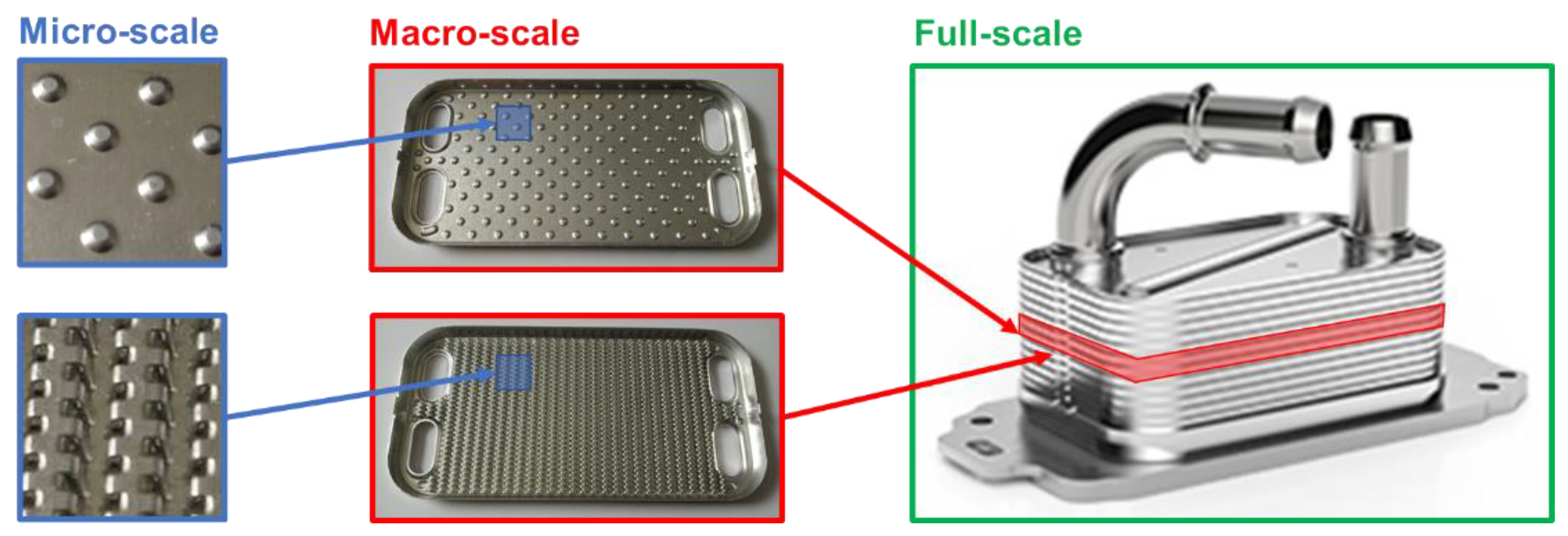
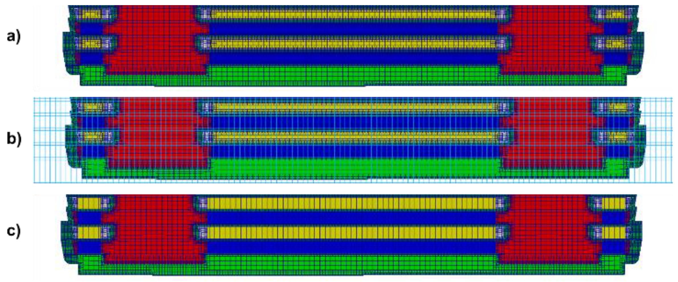
Figure 1 reports an overview of the typical scales, which should be considered to address the simulation of an heat exchanger: (a) The micro-scale, intended as the scale, which describes the smallest geometrical detail significant for the problem; (b) the macro-scale, where the smallest geometrical details of the microstructure are neglected and suitable models are introduced for the description of the average behavior of the porous media; (c) the full-scale, which considers the overall device in its complexity at the largest scales, while the smallest scales are modeled.
Having clear the multi-scale nature of the problem it is possible to setup the full-scale simulation of the device resorting to upscaling strategies. In this context, the upscaling concept consists of performing separate analyses at the different scales, considering for each scale a domain extension, which is representative for the description of the problem. This leads to the definition of a representative elementary volume (REV) for each scale, implying that small scales can be analyzed considering small domains i.e., the higher computational burden related to the high resolution is partially compensated by the smaller domain extension in such a way to limit the overall number of cells. In this framework, the results obtained at the smallest scales can be processed to obtain correlations, for example in terms of pressure drop and heat transfer properties, which can be applied for the modeling of the big scales. This upscaling approach makes it feasible to address the full-scale simulation of complex problems, since at each step only the large scales are resolved while the small ones are modeled, keeping acceptable the computational burden.
2.1. Governing Equations
The modeling of the heat-transfer problem requires us to consider a proper set of governing equations for the two different phases, fluid and solid, involved in the process. In particular, the fluid flow can be described by the following set of equations:
Conservation of momentum:
The constitutive equation of the fluid can be expressed, under the assumption of Newtonian fluid, as:
The set of equations is then closed by the equation of the state of the fluid, which relates the density to the thermodynamics conditions:
Considering the solid phase, the thermal balance is solved considering the conservation of energy:
2.2. Micro-Scale Model
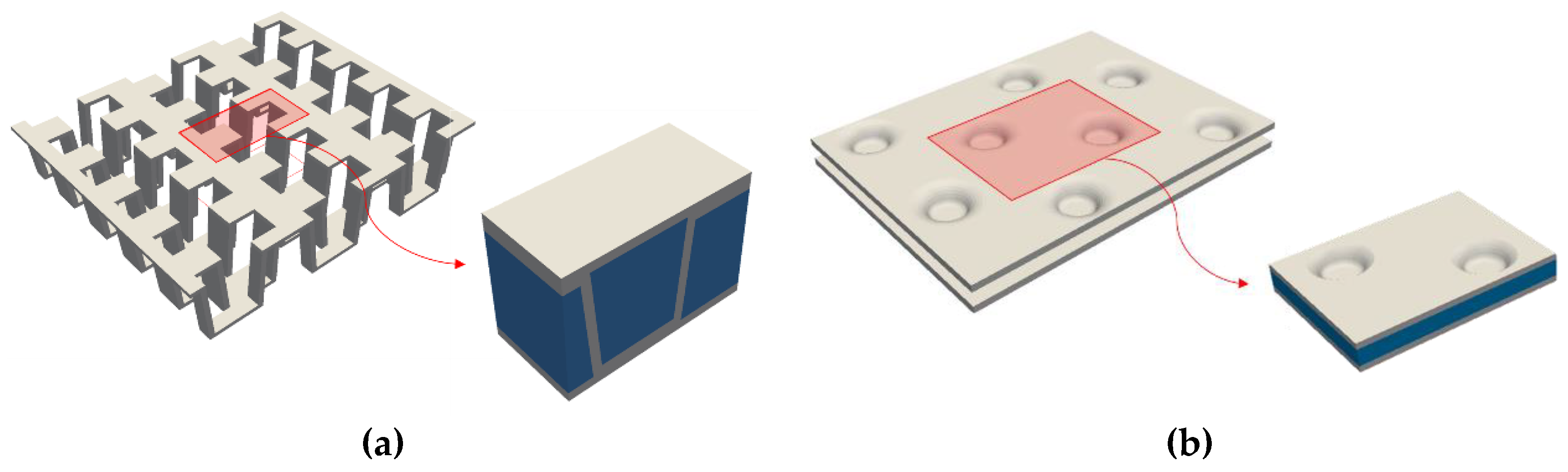
The REV at the micro-scale is defined considering the geometrical periodicity of the turbulator structure, being indifferently based on offset-strip fins or dimples. The model is built on the basis of one single REV, applying periodic conditions at the boundaries of the domain (
Figure 2). It consists of two regions, namely solid and fluid, suitably coupled at the solution level to realize a conjugate heat transfer framework, where heat fluxes are consistently transferred from one phase to the other [
15].
The model is based on Equations (1)–(3), where proper source terms are introduced in order to establish the fluid flow and the heat transfer, due to the presence of cyclic boundary conditions. In particular, the source term on the momentum equation determines the flow velocity in the cyclic domain by mimicking the effect of a pressure gradient. This source term can be expressed as follows:
where
is the desired average flow velocity and
is the direction of application of the volume force. The value of
is determined by an iterative procedure, adjusting its value to target the objective average velocity
. Similarly, a source term on the fluid energy equation is introduced on the basis of the heat flux to be established from the fluid to solid domain:
The thermal setup is completed by the application of a fixed temperature condition at the top/bottom wall of the solid domain and by the introduction of the conjugate heat-transfer condition at the fluid–solid interface. The latter imposes the temperature
on the boundary patch of each region, taking into account temperature and conductivity of the other region, according to the following relations:
where, for fluid and solid regions respectively,
and
are the distances between cell center and face center at the boundary patch,
and
are the temperatures in the cell centers and
and
the conductivities.
The thermo-fluid-dynamic problem at the micro-scale can be described resorting to different levels of approximation. The most straightforward approach consists of adopting a Reynolds Average Navier–Stokes (RANS) approach, where the macroscopic effects of the turbulent phenomena occurring at the smallest length and time scales are included by means of suitable turbulence models. This approach represents an optimal choice when the characteristic size of the geometry is clearly distinguished from the characteristic length scale of the middle-size turbulent vortexes. On the other hand, it may happen that the characteristic size of the geometry is comparable with the size of the vortexes: In this case the grid resolution required for the description of the geometry is enough to resolve also the largest size of the turbulent vortexes. In this case, a large eddy simulation (LES) approach becomes a reasonable option, allowing the direct simulation of the biggest vortexes and introducing a suitable subgrid model for the modeling of the turbulent structures characterized by a size smaller than the grid one. The applicability of the RANS or LES approach is strongly dependent on the specific micro-structural geometry of the turbulator and on the flow regime to be simulated. In particular, in this work, the RANS approach was adopted for the simulation of dimple-type turbulator, while the LES approach was found to be the best choice for the offset-strip fins one. This choice was motivated by the fact that the offset-strip fins structure consists of elements, namely the fins, which are characterized by a thickness, which is critically low (0.1–0.5 mm). In this case, the accurate reconstruction of the fin geometry requires a sufficiently refined grid, which is also appropriate for the resolution of the bigger turbulent vortex according to a LES approach. On the other hand, the dimples have usually a typical diameter of one order of magnitude higher (1–5 mm) and, therefore, the level of refinement required for an accurate reconstruction of the geometry is not enough for the LES, so the RANS approach is preferred.
In the case of the RANS approach and, in general, for all the laminar regimes, where it is possible to obtain a steady-state solution for the physical problem, steady-state simulations are run on the basis of the Semi-Implicit Method for Pressure Linked Equations (SIMPLE) [
19] algorithm up to convergency. On the other hand, when the LES approach is applied, unsteady simulations based on the Pressure-Implicit with Splitting of Operators (PISO) [
20] algorithm are performed, in order to have a full description of the effects of the turbulence on pressure drop and heat transfer. For all the considered Reynolds numbers, different directions of application of the momentum source are imposed to assess a complete characterization of the effects of the flow angle on the turbulator behavior.
The results of simulations can be processed to obtain non-dimensional coefficients of pressure drop and heat transfer, along with their functional dependence on the flow angle
and the Reynolds number, defined as:
where
is the average flow velocity and
is the characteristic dimension of the turbulator geometry. This is computed resorting to different definitions in the case of offset-strip fins or dimple-type turbulator; for the former, the definition of hydraulic diameter is adopted:
while, for the latter, the height of the channel is considered:
On the basis of the simulation results, the friction Fanning factor is obtained as:
where
is the pressure gradient across the sample. On the other hand, Colburn factor is evaluated as:
where the Nusselt number is computed from the heat transferred from the fluid to the solid at the interface
, the fluid bulk temperature
, the solid wall temperature
and the size
of the REV:
2.3. From the Micro-Scale to Macro-Scale Model
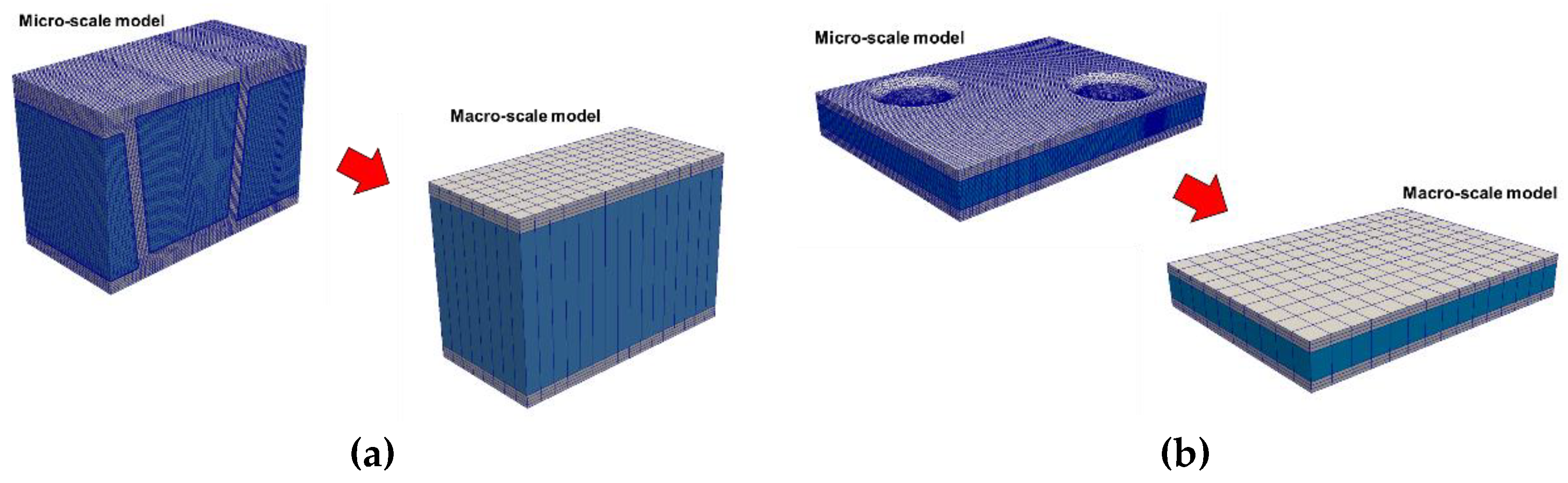
The macro-scale model is derived by means of an upscaling process involving the pressure drop and heat transfer properties computed at the micro-scale. In this framework, a porous media approach is adopted to model the region in which the turbulator is located, neglecting the micro-scale geometrical details and describing the phenomena in terms of macro-scale governing equations. The application of the averaging operator on the REV domain leads to the definition of a porous media zone having a single cell in the direction of the height of the channel, making it possible to approximate the flow in the channel as a 2D problem (
Figure 3).
The resistivity introduced by the presence of the turbulator is taken into account by a specific source term on the momentum equation:
This source term is evaluated according to the local Reynolds number and the direction of the flow
with respect to the high pressure drop direction of the turbulator. On the other hand, the modeling of the heat flux between the bulk of the flow and the solid wall is addressed by prescribing locally the convective heat transfer coefficient for the fluid. This possibility is enabled by the fact of having a single cell in the direction normal to the wall, meaning that the temperature value computed in the cell corresponds to the bulk value. Therefore, the heat flux at the wall can be evaluated as:
where the temperature at the boundary is computed on the basis of the Equation (9) substituting
while the convective coefficient
is evaluated on the basis of the Colburn factor dependency on local Reynolds number and flow direction:
2.4. Full-Scale Model
The full-scale model is built considering the two fluid phases involved in the heat transfer process and the solid phase constituting the metal wall of the heat exchanger. The different phases, being fluid or solid, are modeled resorting to separate meshes, which are adjacent and have coincident boundary patches at their interface. The computational grids reconstruct the complex tridimensional features of the device at the biggest scales (i.e., ducts, fluid passages, geometrical details of the case) while embed the definition of suitable porous zones to account for the presence of the microstructure of the turbulator layer. This is described by means of the macro-scale porous media approach introduced in the previous section, which allows us to adopt the 2D approximation for the modeling of the turbulator channel, resulting in a significant reduction of the computational effort. However, this method requires a careful creation of a 2D mesh for the zone where the turbulator is located. This is not a straightforward operation since these zones are connected to the fully 3D zones modeling fluid passages and ducts. This difficulty has been overcome exploiting the concept of cell agglomeration in the regions in which the 2D mesh should be created. In this framework, the mesh generation consists of two steps: (a) Creation of a base standard 3D mesh, by means of a standard mesh generator and (b) agglomeration of the cells in the porous zones, which should be modeled according to 2D approximation.
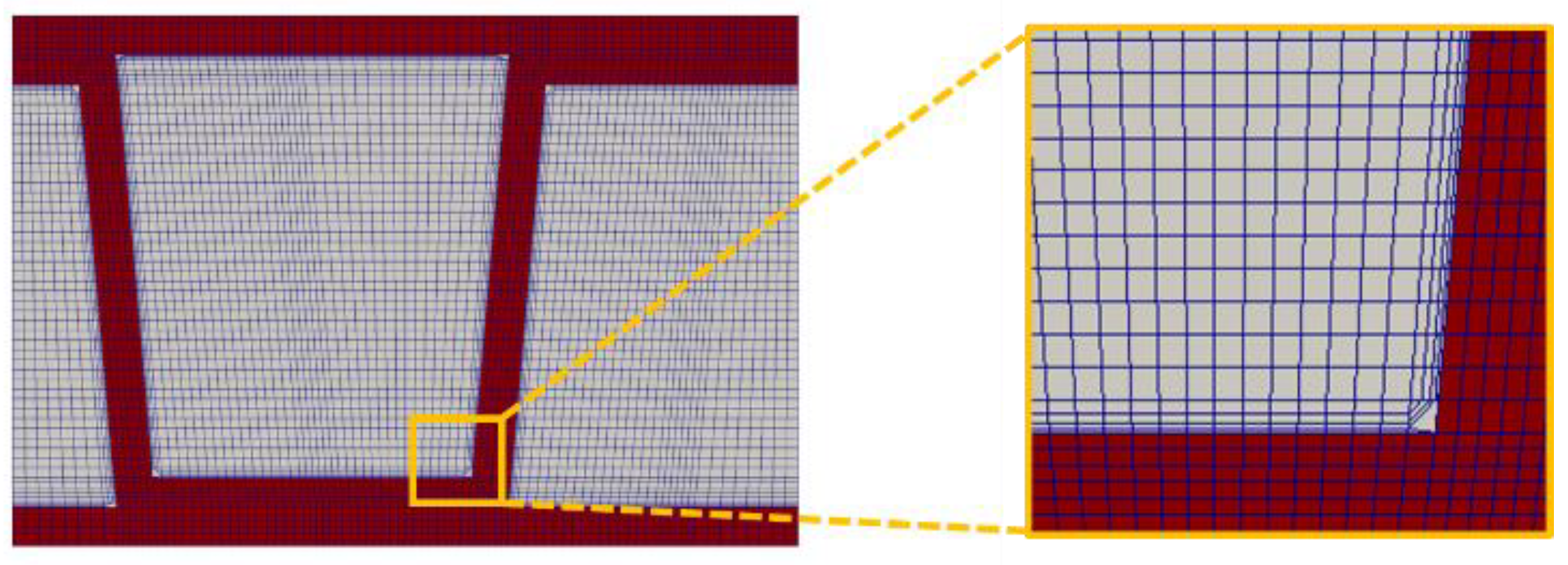
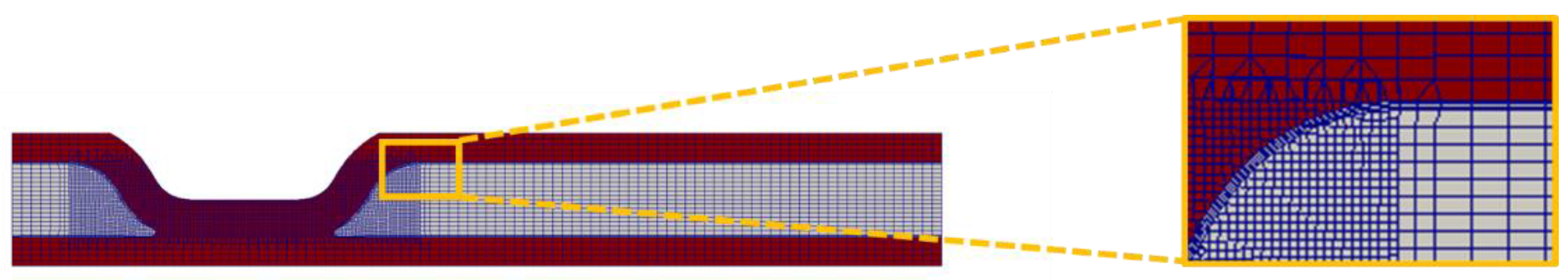
The agglomeration procedure (
Figure 4), whose general concept was detailed in [
21], is based on the adoption of a background agglomeration grid, which defines the desired cell size of the final grid and specifies the cells that need to be merged. The agglomeration process is performed, for each porous zone, merging all the cells of the initial grid, which are located inside the same cell of the background agglomeration grid. The resulting computational grid allows, therefore, to analyze the flow with the necessary level of approximation all over the domain, coupling a fully-3D analysis of the larger scales, represented by the complex geometries of the passages responsible for the flow distribution between the different layers, with an advanced 2D modeling of the turbulator channels, which is governed by the phenomena occurring at the smallest scales.
2.5. Integration between the Different Simulation Scales
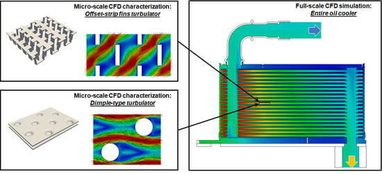
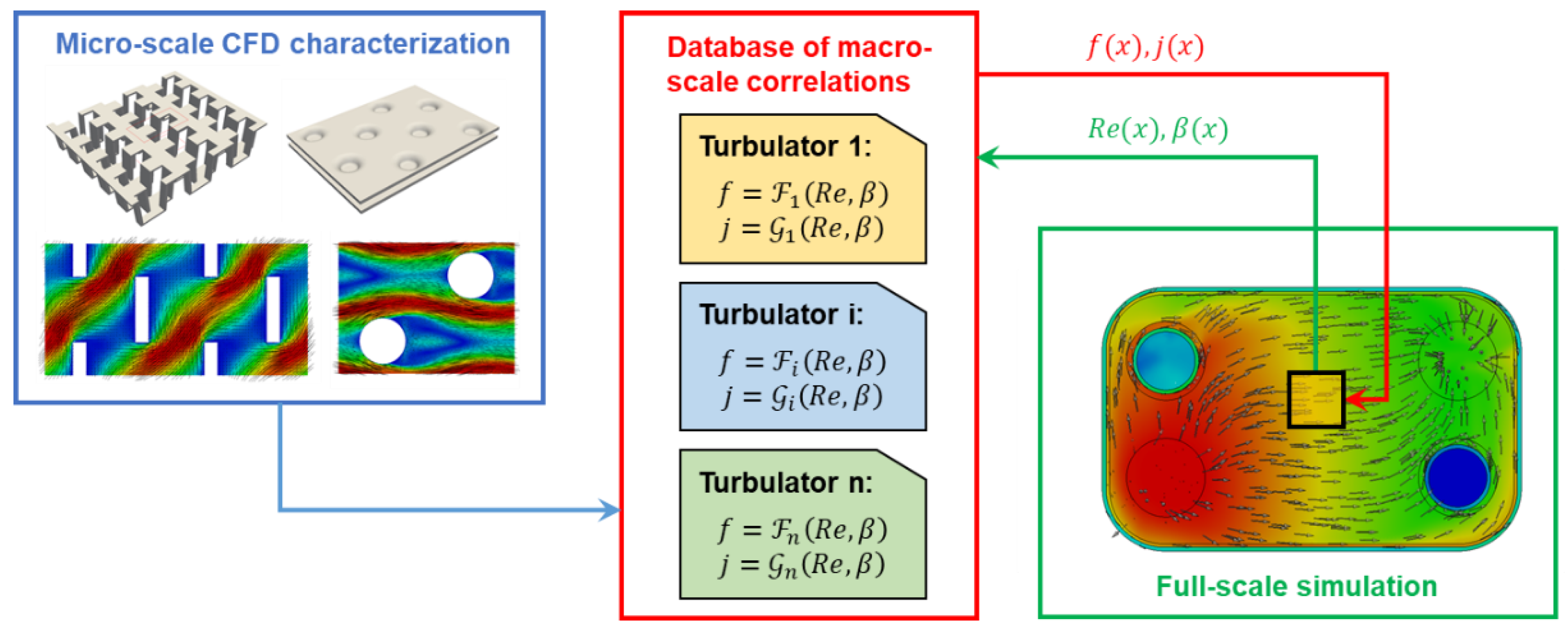
The overall CFD procedure, detailed in the previous paragraphs, is summarized in
Figure 5. In this framework, micro-scale CFD simulations are applied in order to characterize the fluid dynamics and heat-transfer behavior of the turbulator. The procedure can be applied for characterizing different turbulators, in order to build a database for a large variety of micro-structures. The database collects, for each geometry, the characteristic relationship between Fanning/Colburn factors and Reynolds number and direction of the flow, to be applied in macro-scale models. This database provides the basis for the modeling of turbulator regions in full-scale models, employing a macro-scale porous approach. In particular, when full-scale simulation of the cooler is addressed, the pressure drop and the heat-transfer in each location of the turbulator are modeled resorting to the database of correlations. These provide an estimation of the Fanning/Colburn factors on the basis of the local conditions in terms of Re and β calculated in each computational cell, which discretize the porous turbulator region. In case of the presence of different types of turbulators in the cooler, the appropriate correlation is selected.
4. Results and Discussion
The simulation of the oil-cooler performance was addressed on the basis of the multi-scale approach described in the previous section: At first, a detailed micro-scale analysis was applied to characterize the turbulator behavior and, then, these results were upscaled and adopted in the macro-scale models. This allowed us to perform the full-scale modeling of the heat exchanger, taking into account all the significant phenomena occurring at the different scales and providing a reliable characterization of the performances of the device.
4.1. Micro-Scale Offset-Strip Fins Turbulator Characterization
The modeling process started with the generation of the multi-region mesh for the characterization of the turbulator performances. The extension of the computational domain was reduced to a single REV adopting cyclic boundary conditions at the boundaries, in such a way to reduce at the minimum the number of cells needed for the analysis. The computational grid (
Figure 7) consists of a block-structured fully-hexahedral mesh, whose mesh size is chosen on the basis of the maximum Re number to be simulated, in order to allow the description of the turbulent regimes according to a large eddy simulation (LES) approach. To this purpose, maximum grid size is selected on the basis of the Kolmogorov length scale
, according to:
For the present calculations a factor was considered, meaning that at the highest Re the smallest resolved scale was 10 times the Kolmogorov one. The resulting grid was characterized by an average cell size of 40 μm, which was further refined at the wall, and consisted of a total cell number of cells for the fluid domain and cells for the solid one.
Simulations were run in order to characterize the overall range of
Re numbers and flow angles. At low Re numbers (
Re < 100) steady-state SIMPLE simulations were run up to convergency. For each simulation, convergency is considered achieved when the initial values of the residuals fall below appropriate thresholds for all the governing equations. On the other hand, for high Re numbers, especially in combination with small flow angles, it is not possible to obtain physical convergency to a steady-state solution. In this case, the flow fields are locally characterized by unsteady periodic oscillations, related to the anisotropic nature of the turbulator. As a matter of fact, the flow tends to deviate according to the direction parallel to the turbulator, in such a way to reduce the pressure drop, and inverts periodically the angle in order to maintain the imposed average flow direction. Therefore, the Implicit Large Eddy Simulation (ILES) approach was adopted to describe these regimes: In this way the large turbulence scales are fully resolved while the dissipative effect of the smallest ones is taken into account by the numerical diffusion related to the adopted numerical schemes. In this case, second order accurate linear schemes were applied for both space and time discretization.
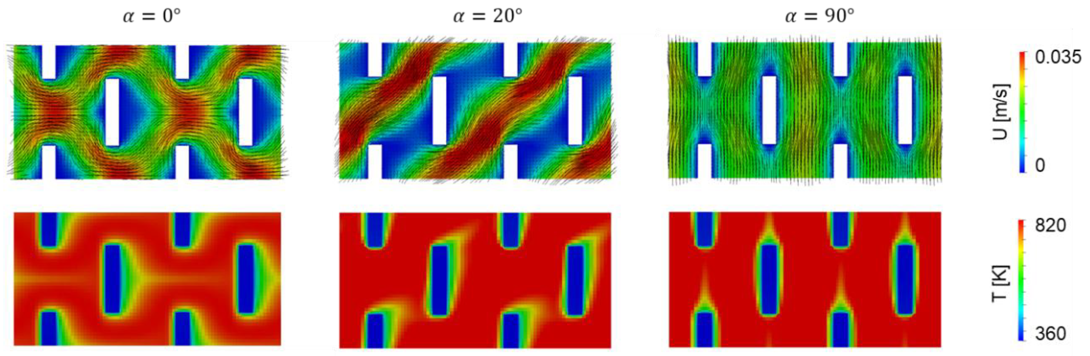
Figure 8 reports the computed velocity and temperature fields for average velocity equal to 0.01 m/s and for different angles
α of application of the momentum source. In this case no unsteadiness was recorded due to the low
Re number, which characterized the flow. It is possible to notice that, considering an intermediate angle
α of application of the momentum source (i.e., direction of the pressure gradient) the resulting angle
β of flow tended to increase due to the anisotropy of the turbulator structure. For example, in the reported flow field, pressure gradient angle α equal to 20° corresponds to a resulting angle
β of the flow around 45°.
Figure 9 reports the evolution of the velocity and temperature fields considering a turbulent regime (
U = 2 m/s) and an angle
β equal to 0°. In this case, periodic oscillation of the flow direction around
α = 0° were registered, in order to minimize the overall pressure drop.
To fully characterize the turbulator behavior, micro-scale simulations were run with an automatic procedure covering all the possible operating conditions, which can be established in the typical operation of the device. In particular, the Re number and flow direction
β were assumed as input variables for the analysis and were varied according to the full factorial design of the tests, considering 11 levels for
Re and seven levels for
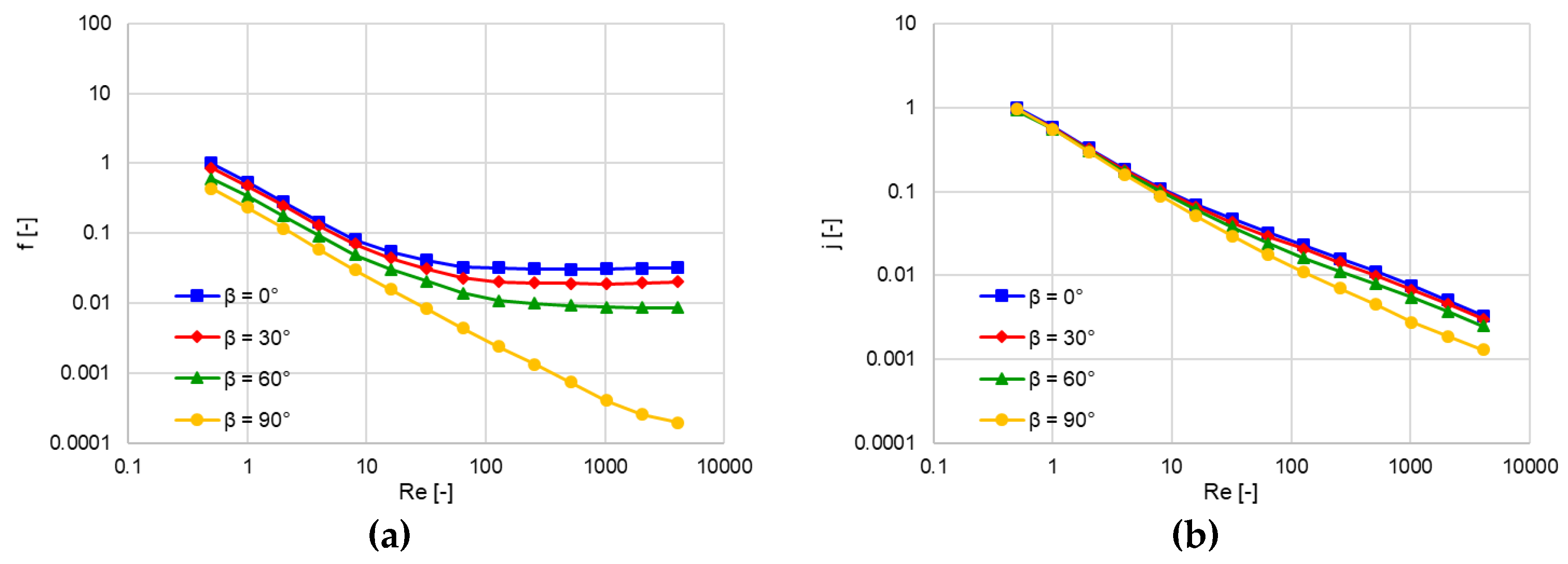
β, resulting in total 77 points. The simulations provided the response of the CFD model in terms of pressure drop and heat transfer for each operating point. These results were then processed in order to compute Colburn and Fanning factors. Hence, two-dimensional interpolation was applied in order to provide correlations describing the relationship between Colburn and Fanning factors and the variables on which they depend, namely Reynolds number and flow angle. These are shown in
Figure 10. Typical trends reported in the literature [
3] are recovered, showing a clear transition between laminar and turbulent regimes for a critical
Re number variable between 10–1000 depending on the flow angle. In particular, small flow angles
β promote an earlier transition to turbulent regime, resulting in a significantly higher pressure drop and slightly enhanced heat exchange properties for the same average
Re.
The steady-state characterization of each point, performed with the SIMPLE algorithm, requires a computational time of less than one hour on a single processor, considering a standard workstation. The computational time significantly increases when transient LES simulations are performed, with maximum runtime around 24 h for each point. In order to minimize the overall computational time required for the full characterization of the map multi-processor strategy was applied, running the different simulations simultaneously on different processors and, in the second instance, exploiting parallel computing capabilities for running each simulation on multiple processors.
4.2. Micro-Scale Dimple-Type Turbulator Characterization
The characterization of the dimple-type turbulator is addressed with an approach similar to that adopted for the case of the offset-strip fins one. In this case, the two regions mesh is built using an automatic Cartesian mesh generator (snappyHexMesh, a utility included in the OpenFOAM toolbox [
17]), capable to provide a body fitted grid, predominantly hexahedral and including a small percentage of polyhedral elements near the boundary walls. Boundary layers are added near the wall to provide a better description of the fluid-wall interaction in terms of both wall shear stress and heat-transfer. The resulting mesh consists of
cells for the fluid domain and
cells for the solid one (
Figure 11).
Turbulence modeling was addressed with a RANS approach employing k-ω Shear Stress Transport (SST) model [
22]. Steady-state simulations were run on the basis of the SIMPLE algorithm considering different
Re numbers and flow angles.
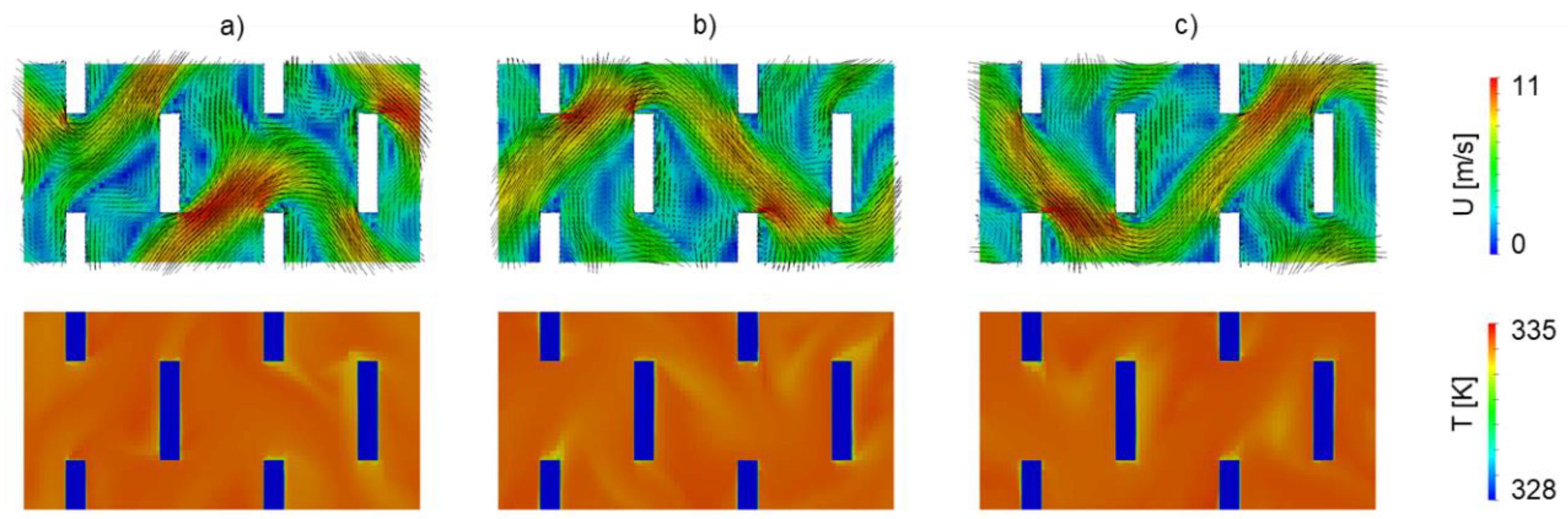
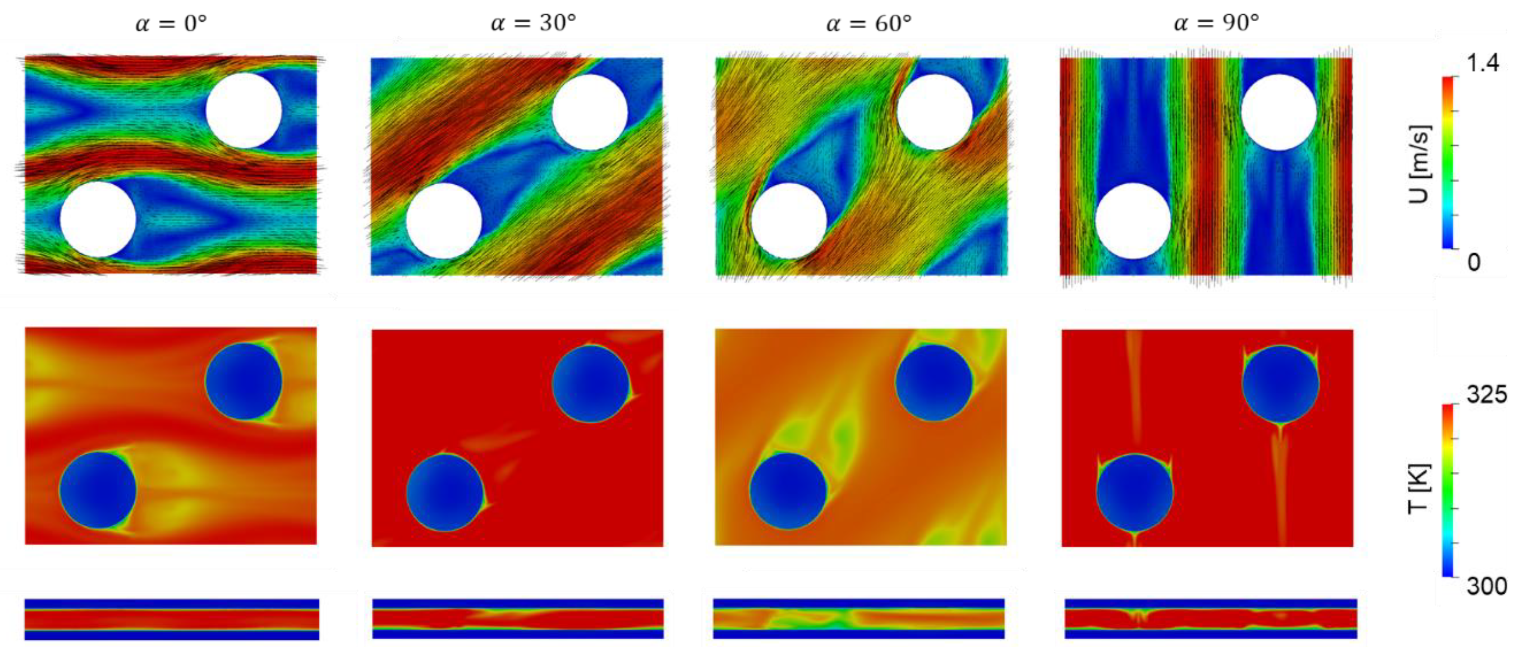
Figure 12 reports the computed velocity and temperature fields for an average velocity equal to 0.5 m/s and different angles α of application of the momentum source. It is possible to notice that, in the case of dimples, the angle α of application of the momentum source (i.e., direction of the pressure gradient) is quite correlated to the resulting angle
β of the flow, due to the low grade of anisotropy of the turbulator structure (i.e., different pitch between dimples in the x and y direction). This behavior was significantly different with respect to the case of the offset-strip fins turbulator, where the flow direction was strongly influenced by the fins orientation. However, depending on the flow angle, the dimple array had a different influence on the enhancement of the flow mixing. For instance, for the reported flow field, the pressure gradient angle α equal to 30° and 90° determined a flow stream that was perfectly aligned with the dimples, with large wake regions that reach the dimple located downstream: This determines a low impact in promoting the mixing. On the other hand, α equal to 60° was more effective in this sense, since each dimple was reached by a high velocity flow stream, which was split and deviated towards the following dimple. This enhanced the heat transfer since the front of each dimple was always invested by a high temperature stream. Moreover, downstream the dimples, strong recirculation zones were induced. Similar effects could be noticed also in the case of α equal to 0°, where the adopted ratio between dimples pitch in the longitudinal and transversal direction was particularly effective in promoting the heat transfer.
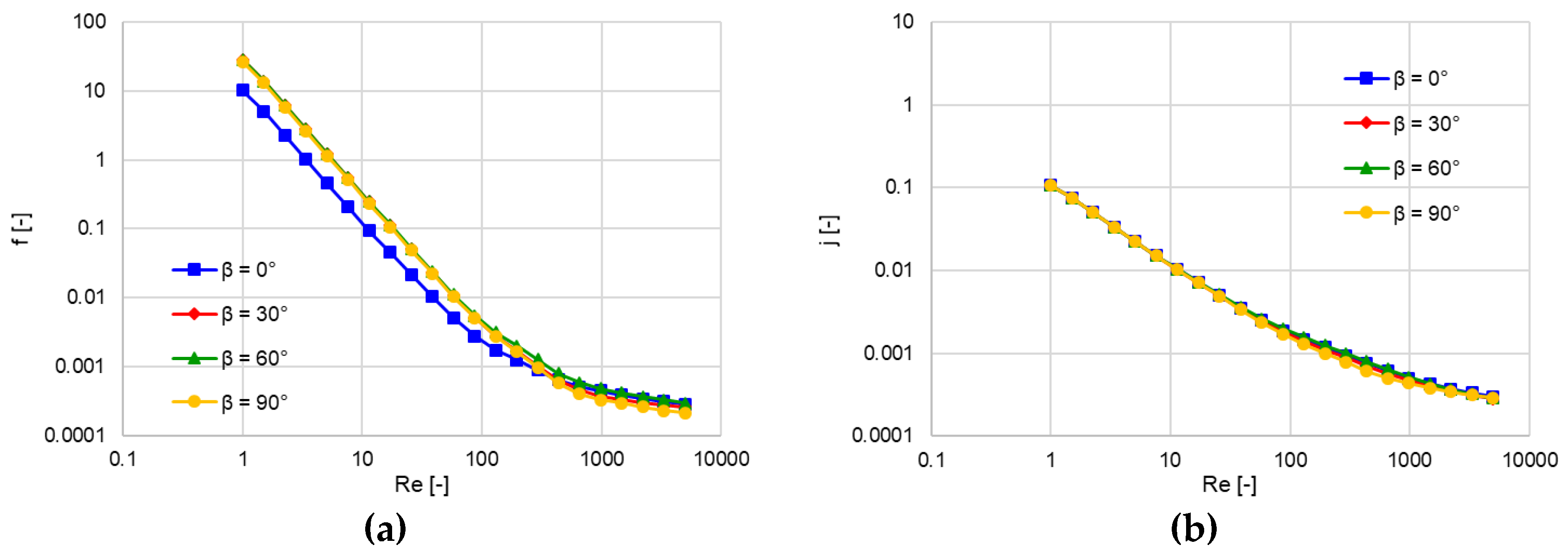
The dimple-type turbulator behavior was characterized simulating different operating conditions with
Re number in the range between 0–2000 and at four different flow direction
β. These results were processed by applying 2D interpolation and extracting the maps of Fanning and Colburn factors, as reported in
Figure 13. As already noticed in case of the offset-strip turbulator, a clear transition between laminar and turbulent regimes can be identified. However, the dependency of the factors on the flow angles
β was negligible: Only the friction coefficient in case of
β = 0 was halved with respect to the values at higher angles. Compared to the offset-strip fins, the dimple-type turbulator exhibited, in the laminar regime, higher friction coefficients and lower heat-transfer ones. This was confirmed also for what concerned the Colburn coefficient at the high
Re. On the other hand, at high
Re numbers Fanning factor for dimples did not depend on the flow angles
β and it was generally lower with respect to offset-strip fins.
4.3. Full-Scale Cooler Simulation
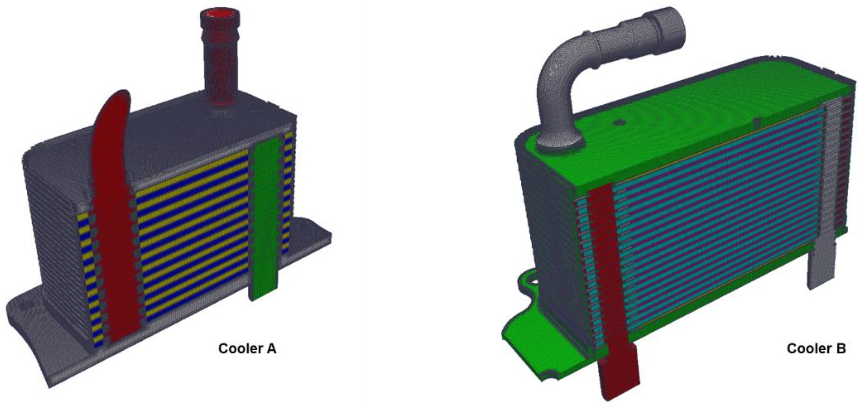
Once the micro-scale behavior of the turbulator was fully characterized, extracting macro-scale pressure-drop and heat-transfer correlations, the modeling of the overall cooler configurations was addressed. The computational grids are shown in
Figure 14: these consist of three regions (coolant, lubricant and metal case) and include porous zones where cells are agglomerated in order to apply the macro-scale turbulator model. The base mesh is generated with an automatic Cartesian mesh generator (snappyHexMesh [
17]), obtaining a grid predominantly hexahedral, with a small percentage of polyhedral elements near the boundary walls. The mesh was then agglomerated according to the strategy described in a previous section. The resulting mesh of cooler A consisted of
cells for the coolant region, of
cells for the oil region and
cells for the solid one. The cell count for cooler B was
cells for the coolant region,
cells for the oil region and
cells for the solid one. It can be noticed that the discretization of the solid region requires a significantly high number of cell with respect to the fluid ones: This is due, on one hand, to the geometrical complexity and to the thinness of the metal walls and, on the other hand, to the fact that the fluid regions include large zones in which cells have been agglomerated. However, it should be considered that the solution of the solid region requires lower computational resources with respect to the fluid ones, since a single governing equation has to be solved, namely the heat balance. Therefore, the high number of cells in the solid region is not usually a limiting factor for what concerns the computational effort.
Steady-state multi-region conjugate heat transfer simulations were run applying the SIMPLE algorithm on the fluid regions. Thermal coupling between regions was achieved by means of the boundary conditions described in a previous section. The modeling of porous regions was performed on the basis of the correlations extracted by means of the detailed micro-scale analysis of the REV. The turbulence occurring in the device, especially in the large flow passages and inlet/outlet ducts, was described by means of the k-ω SST turbulence model. Conversely, in the porous regions, where the turbulence effects, if present, are already included in the pressure drop and heat-transfer correlations, the turbulence level is dropped down applying specific source terms.
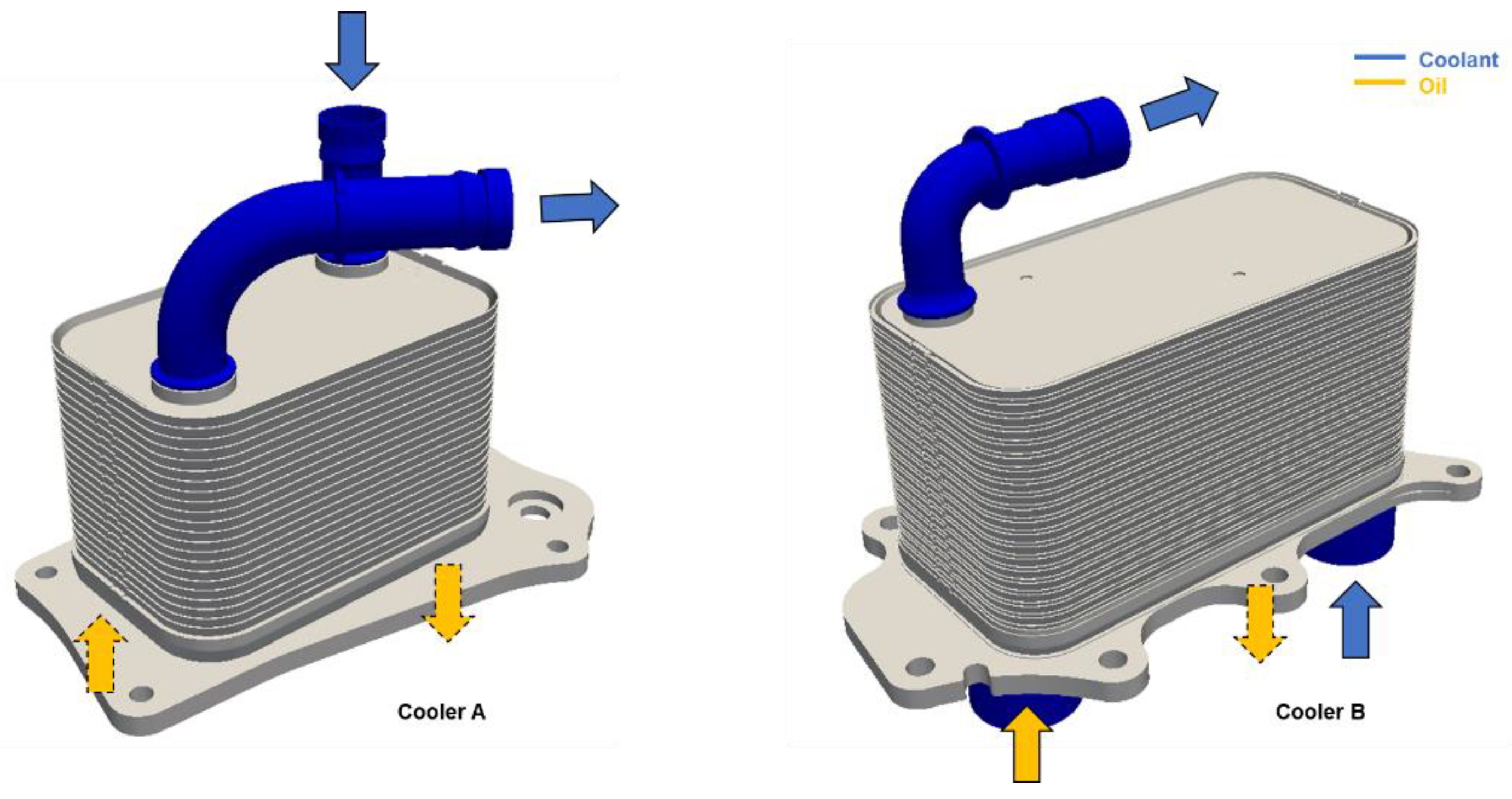
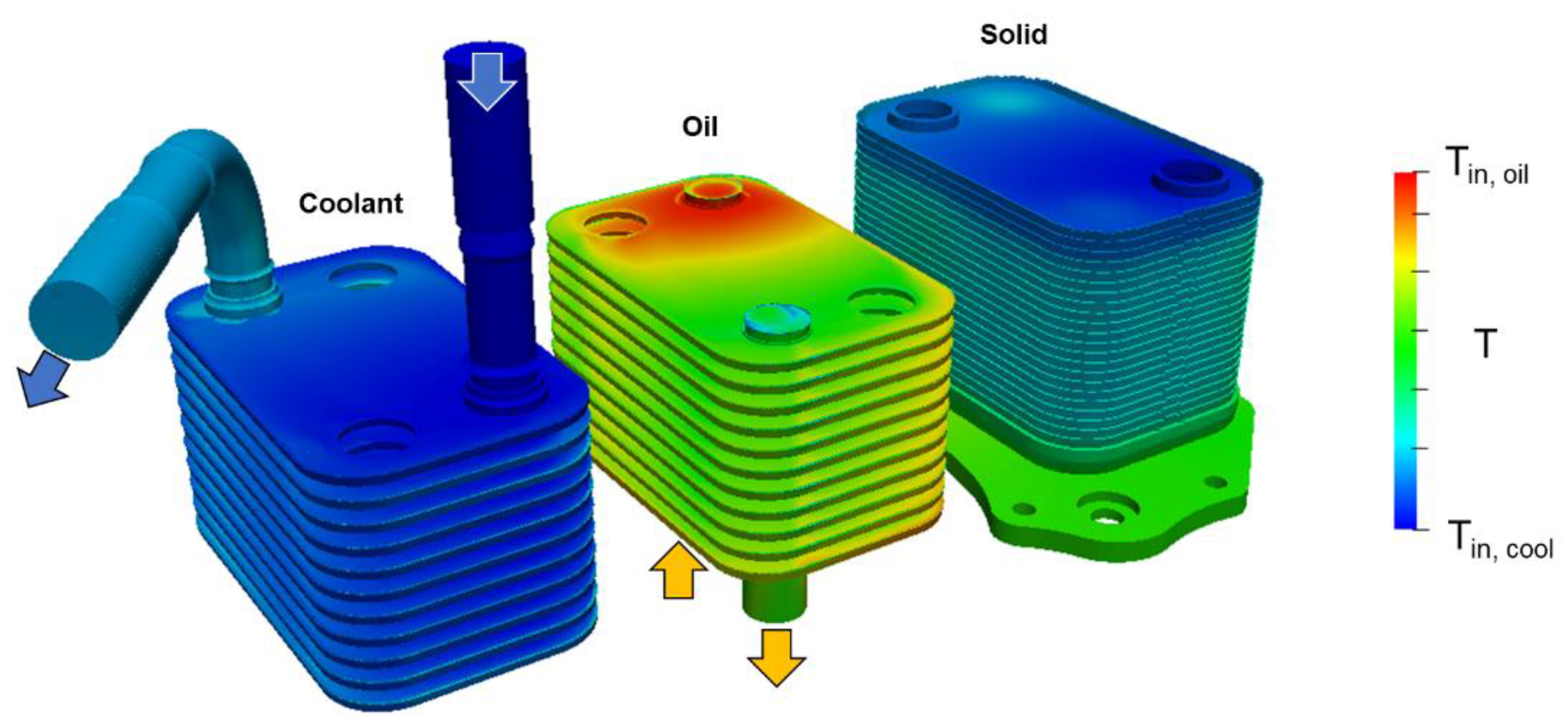
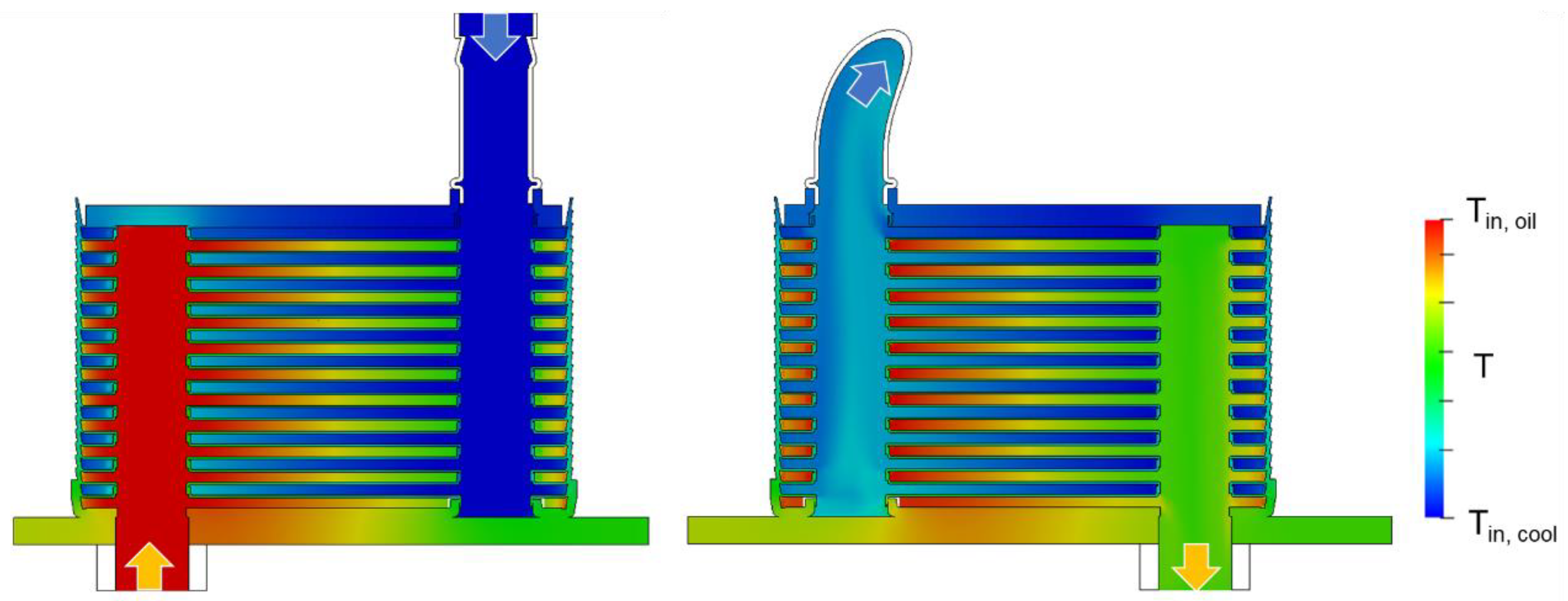
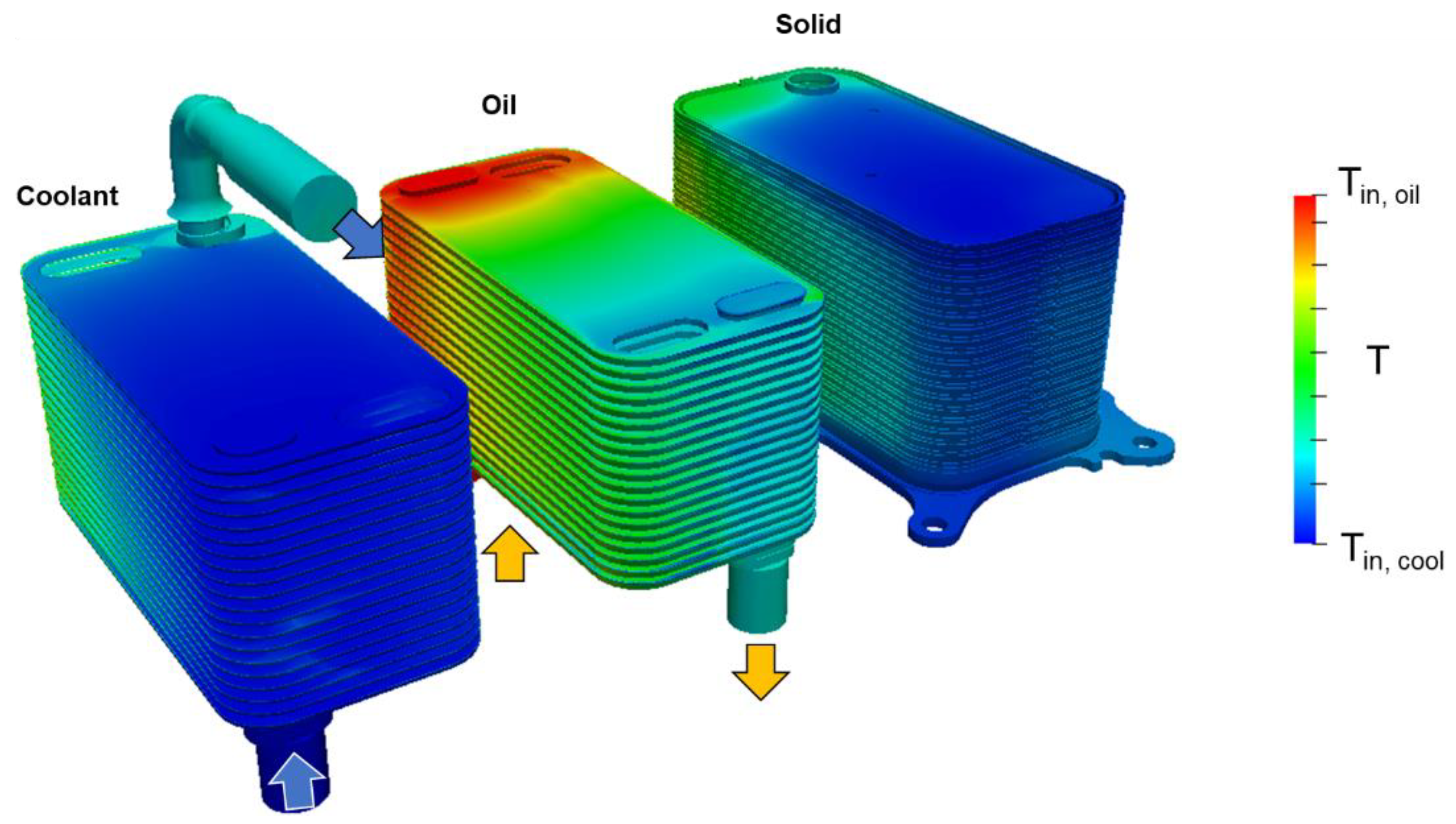
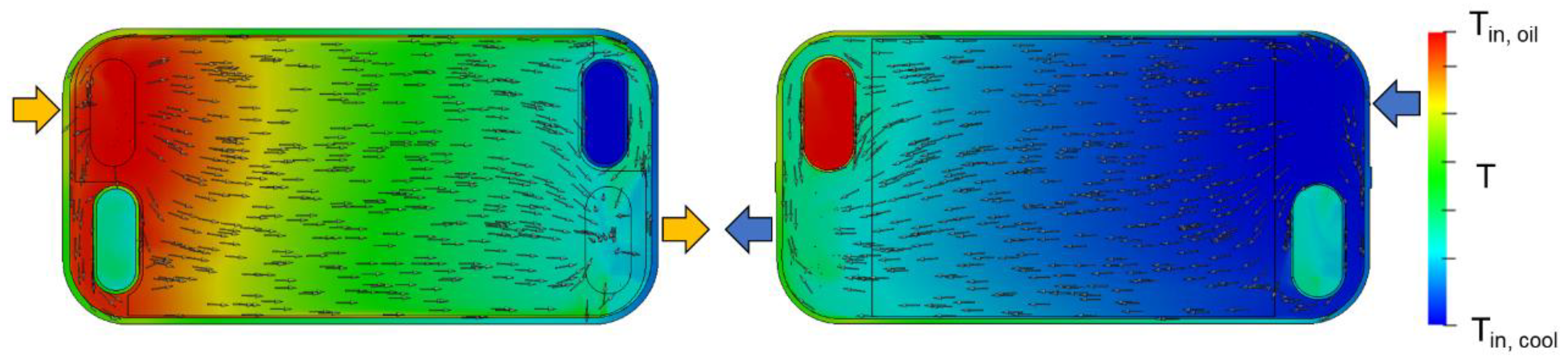
Figure 15 reports the temperature field in the different fluid and solid regions computed for cooler A considering one of the simulated operating conditions. It can be seen that the cooler operates as a counterflow heat exchanger, with the inlet and outlet of coolant and oil located in the opposite position. Moreover, the temperature of the metal casing shows the lowest values at the top, where it is in contact with the coolant layer, while the highest temperatures are located in the bottom part.
The temperature evolution of the two fluids flowing in the cooler can be investigated considering two longitudinal cross sections passing through the inlets and the outlets, as shown in
Figure 16. This view highlights that the temperature evolution is quite similar for all the corresponding oil or coolant layers, with the exception of the top and the bottom one. In this case the peripheral layers can exchange heat just on one side and, therefore, their contribution to the overall heat transfer is penalized with respect to the central ones. This suggests that the adoption of specific low permeability turbulator for the oil layer could improve the overall heat transfer balancing among the different cooler passages.
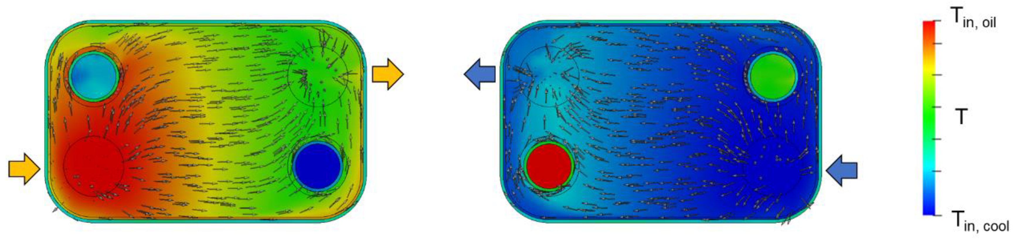
Figure 17 shows the temperature evolution of oil and coolant considering two intermediate passages located in the middle of the cooler. For the considered operating condition (Q
oil = 50%, Q
cool = 80%), the temperature increase of the coolant was quite limited while the oil temperature drop was more significant, due to the ratio between the two flow rates. Moreover, considering the flow direction in the passages, it could be noticed that the presence of the turbulator forces the flow to align with longitudinal direction of the heat exchanger in the central part, while a significant redistribution of the flow occurred near inlet and outlets.
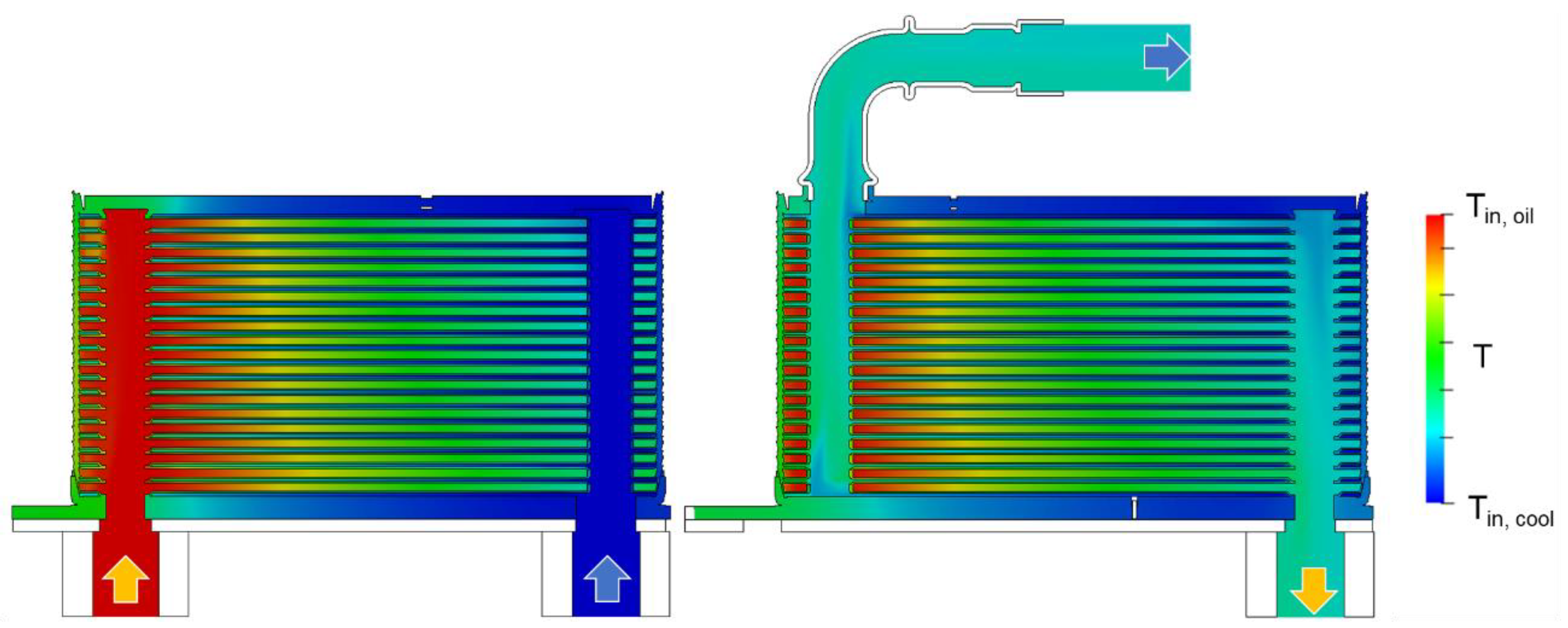
Simulation results for cooler B are reported in
Figure 18,
Figure 19 and
Figure 20. Despite the different design of this cooler, which adopt dimples instead of offset-strip fins on the coolant side and includes a higher number of layers, the overall evolution of the fluid temperature was qualitatively similar to what was already described for configuration A. However, a better oil cooling was ensured by the fact that oil layers were one less than coolant layers, allowing a more effective cooling at the top and bottom side. Considering the transversal section of the oil and coolant passages located in the middle of the heat exchanger, it can be noticed that, in the case of the oil layer, the flow in the central part is perfectly aligned with the longitudinal direction due to the presence of the turbulator. On the other hand, for the coolant layer, a little deviation in the direction of the inlet–outlet connecting diagonal was observed, as a consequence of the quasi-isotropic behavior of the dimple microstructure.
For both the coolers, simulations were run in parallel on six processors, applying domain decomposition on all the three regions. Simulation convergency was generally achieved, for all the operating conditions considered, in a maximum 12 h of computational runtime.
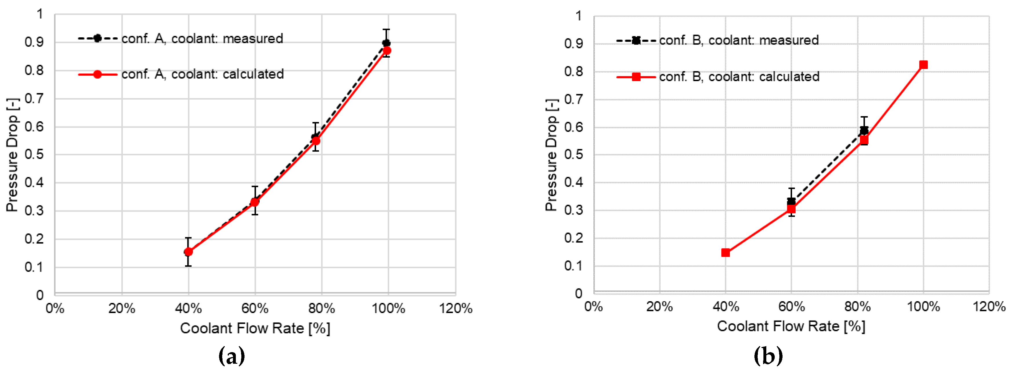
Figure 21 reports the pressure drops computed for the coolant side of the two configurations, along with the corresponding measured values. The pressure drop was evaluated, both in the experiments and in the simulations, at the inlet and outlet sections of the cooler, including therefore also the effect of the connecting bended pipes (
Figure 6). It is worth highlighting that configuration A is equipped with offset-strip fins turbulator while configuration B includes dimple-type turbulator. The agreement between simulations and measurements could be judged as satisfactory, since the maximum error was below 5% (computed with respect to the maximum value of the dataset). Despite the different turbulator type, the pressure drops of configurations A and B were similar: This was due to the fact that the higher number of layers of configuration B compensates the higher Fanning factor of the dimples with respect to the offset-strip fins.
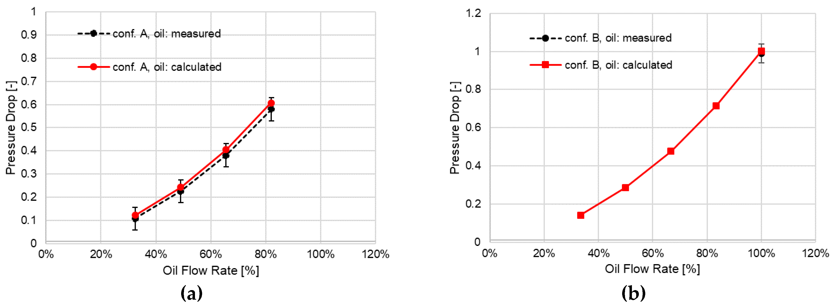
Pressure drop on the oil side are reported in
Figure 22. Configuration B was able to work with the highest maximum oil flow rate, for which the maximum pressure drop was registered. Moreover, comparing the pressure drop for intermediate flow rate, it could be observed that the values for cooler B were slightly higher, despite the higher number of layers: This was because of the different height of the turbulator channel, which was 20% higher in the case of cooler A.
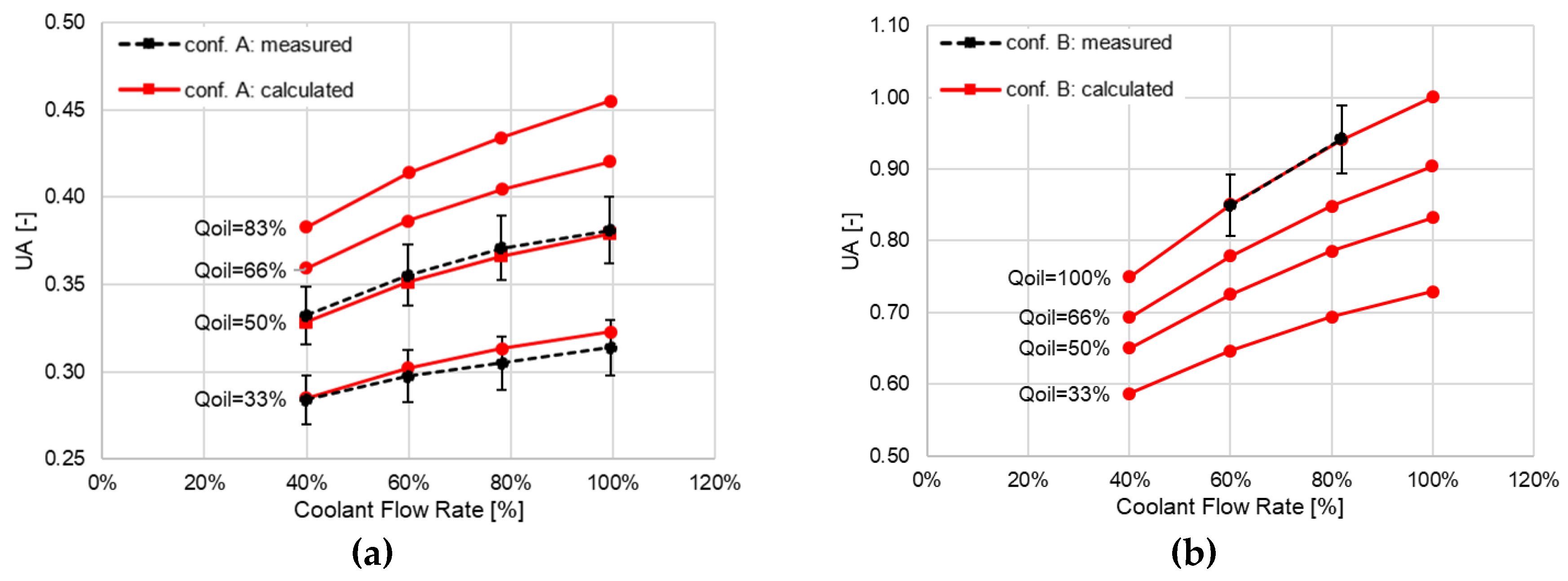
The overall heat transfer coefficient
of the two coolers, evaluated on the basis of the exchanged thermal power and the logarithmic mean temperature difference between the oil and coolant streams, is shown in
Figure 23. The comparison between calculations and measurements shows a reasonable agreement for the available measured points, with the heat transfer coefficient, which increased with both coolant and oil flow rates. Moreover, comparing the two coolers, it could be seen that cooler B had a better performance in terms of heat transfer, reaching
coefficients around two times higher than those of cooler A. This was due to the higher dimensions and to the higher number of layers of the second cooler.
5. Conclusions
In this work the development of a CFD model for the simulation of plate heat exchangers equipped with turbulators was reported. The modeling concept was based on a multi-scale approach: In this view, simulations were run at the smallest scales in order to derive the correlations that would be exploited for the simulation of the biggest scales. In particular, the two main scales, namely micro-scale and full-scale, were considered. At first, the behavior of the turbulators, in terms of pressure drop and heat transfer, were fully characterized with micro-scale simulations, generating suitable maps of Fanning and Colburn factor as a function of the average Re number and flow angle. Then, these maps were employed in the macro-scale model of the turbulator, which was included in the full-scale model of the heat exchanger.
The simulation methodology was tested considering two cooler configurations, with different characteristics in terms of dimensions, number of layers, type of turbulators (offset-strip fins and dimples) and positions of fluid connections. The comparison with experimental measurements had shown an overall satisfactory agreement in terms of pressure drop and heat transfer for a wide range of operating conditions. The approach was exploited to obtain a valuable insight into the details of the heat transfer process, describing the flow distribution between the multiple channels and providing guidelines for a further optimization.
The computational requirements of the model were compatible for running on a standard workstation and the parallel capability allowed us to significantly reduce the simulation runtime. The typical simulation of one operating point could be run over night. Acceptable scalability of parallel computations based on domain decomposition was verified up to 6–10 processors, then, for the cell count considered in this work, performances underwent degradation due to the increase of the weight of processor to processor communications.

 ,
, 


