Evaluation of Energy-Environment Efficiency of European Transport Sectors: Non-Radial DEA and TOPSIS Approach

Abstract

Transport is recognized as a major energy consumer and environment pollutant. Recently scholars have paid considerable attention to the evaluation of transport energy and environmental efficiency (EEE). In this paper, the non-radial Data Envelopment Analysis (DEA) model was employed to evaluate EEE on a macro level—i.e., of European road, rail and air sectors. The evaluation was conducted under the joint production framework, which considers energy and non-energy inputs, and desirable and undesirable outputs for the last ten years period. To rank decision-making units and check the aptness of this non-radial DEA model in transport EEE evaluation, the Technique for Order of Preference by Similarity to Ideal Solution (TOPSIS) method has been proposed. An empirical study has been conducted for as many European countries as possible, depending on availability of data. Based on the non-radial DEA model, it could be said that the level of EEE is improving for the road sector, while many evaluated countries have low EEE for the rail transport sector. Additionally, results have indicated that the TOPSIS method is more suitable than the non-radial DEA model in transport EEE evaluation and for identification of best practices.

1. Introduction

1.1. Background

During recent decades, there have been increased debates concerning the gradual increase of global warming and the resulting climate change. The primary sources of global warming are increased concentrations of greenhouse gas (GHG) emissions, primarily carbon dioxide (CO₂), which is a product of human activities. The transport sector is one of the inevitable and essential parts of human activities, backbone of the economy, representing advantages for society in terms of transportation of goods and people, market integration, and provision of growth and jobs. It has been estimated that transport sector within the European Union (EU) contributes for 7% of European gross value added and 7.06% of employment [1].

Yet despite benefits, transport activities include disadvantages related to responsibilities for enormous energy consumption and resulting GHG emissions. According to the European Environmental Agency [2], with 348.5 Mtoe (Million tonnes oil equivalent), the transport sector was the biggest energy consumer in 2013, followed by households (295.9 Mtoe), industry (276.6 Mtoe), services (152.5 Mtoe) and fishing, agriculture, forestry and non-specified (30.2 Mtoe). Among transport modes in 2012, road transport had the largest share in the amount of consumed energy (307.5 Mtoe), followed by air (international and domestic) transport (51.5 Mtoe), international marine bunkers (46.4 Mtoe), rail transport (7.2 Mtoe), and domestic navigation (5.7 Mtoe) [1].

To ameliorate these disadvantages, the European Commission periodically published White Papers and emphasizing where the targets of EU policies were highlighted. The strategy set by the European Commission [3] was based on targets such as:

• Low emissions through reduction of 60% of GHG emissions by 2050 with respect to their 1990 level;
• Improvement of energy efficiency by decreasing final oil consumption and dependency ratio. The reduction was estimated at 12 to 13% by 2030 and to about 70% by 2050;
• Limited growth of congestion due to better multimodal solutions and new technologies.

Presently, the need for meeting the demands of transportation services and enhancing mobility is increasing, as well as the need for improving the EEE [1]. Awareness and concern about the energy consumption and environmental problems are becoming increasingly important worldwide. Numerous techniques have been employed to address the issues related to energy and the environment. The technique, which has received great attention, is the Data Envelopment Analysis (DEA) method as a non-parametric approach to efficiency evaluation [4]. Recognizing the share that transport has in energy and environmental problems, and having in mind the potential of the DEA method in energy-environment efficiency evaluation, DEA has been included in the analysis of transport EEE. The DEA method has been used in EEE analysis for different sectoral levels, countries and regional levels, as well as timely levels [5]. However, EEE evaluation and comparison of transport sectors on a macro level for EU countries is missing. Since the countries of the EU could have different strategies and measures in energy consumption and environment protection, it is of the utmost importance to identify the best practice.

1.2. The Aim and the Scope of the Paper

The aim of this paper is twofold. The first is to evaluate and analyze the changes of EEE of European road, air, and rail transport sectors, where the methodology for evaluating EEE is based on a non-radial DEA model proposed by Wu et al. [6] for 2006–2008, 2010, 2012, and 2014–2016, using the available data for the European countries which represent DMUs. The second aim of the paper is the introduction of the TOPSIS method in the evaluation of EEE, where the TOPSIS method is used for the ranking of DMUs. The evaluation of transport EEE has been done under the joint production framework, using non-energy inputs (labor and transport assets) and energy input (energy consumption) to produce desirable outputs (volume of passenger and freight transport) and undesirable output (GHG emissions). Aside from other widely used non-radial DEA models such as Slack-based models, Russell measure models, and Directional distance function, in this paper, the non-radial DEA model has been chosen due to its ability to use different non-proportional adjustments, with decision maker specified weights assigned to each efficiency score, and because of its ability to proportionally decrease the amounts of energy inputs and undesirable outputs simultaneously as much as possible [5,6].

The main contributions of this study are: (i) a newly systematic literature review in the field of transport EEE evaluation, (ii) a new definition of transport EEE, (iii) the evaluation of EEE with an extended set of used inputs, (iv) the evaluation of EEE of road, air, and rail transport sectors of European countries and their changing tendencies in terms of the EEE, (v) use of non-radial DEA and introduction of the TOPSIS method through DMUs ranking in the evaluation of transport EEE, as well as the comparison of their results and the identification of the most suitable one for the evaluation of the transport EEE. Based on the evaluation with the non-radial DEA model all stakeholders can create a sense of tendencies in terms of EEE of EU transport sectors. Through the introduction of the TOPSIS method for the same purpose, the science community can consider it as a potential tool for monitoring changes regarding EEE.

The following section presents the review of previous papers which have used DEA or TOPSIS methods in terms of transport EEE evaluation. Section 3 describes the methodology and considers which DEA model is appropriate for our purpose as well as the adoption of the TOPSIS method. The data used, DMUs selection, energy input, non-energy inputs, desirable outputs and undesirable output for EU countries are described in the second part of this section. Section 4 offers an overview of inputs and outputs for transport sectors and compares the results produced by non-radial DEA and the TOPSIS method, as well a discussion related to the obtained results. Finally, the summary of this study and some future directions in transport EEE evaluation are presented in Section 5.

2. Literature Review

The aim of the literature review was to perform an overview of papers related to the evaluation of energy efficiency and environment efficiency or both in the field of transport using different DEA models. In addition, a literature review was conducted as a basis for the process of identification of inputs and outputs for the non-radial DEA model. Moreover, a literature review was made in order to confirm the novelty of the introduction of the TOPSIS method in the evaluation and ranking of DMUs in EEE. Consequently, the literature review was focused on identifying the papers related to the evaluation and analysis of transport EEE with the DEA and TOPSIS methods, as well as in their combination.

The search strategy consisted of a literature review of relevant studies published in peer-reviewed journals within scientific sources such as Ebsco, ScienceDirect, Scopus, Springer, and Taylor and Francis, without limitation on the time period of publishing. The search, performed on titles, abstracts, and keywords for English written full-text free-available scientific journal papers, was finished in April 2019. Conference papers, projects, periodicals, and working papers related to this topic were not included in our review because they went through a less rigorous peer-review process. The application of keywords such as “energy efficiency AND Data Envelopment Analysis”, and “environment efficiency AND Data Envelopment Analysis”, “energy efficiency AND Technique for Order of Preference by Similarity to Ideal Solution”, and “environment efficiency AND Technique for Order of Preference by Similarity to Ideal Solution”, as well as the combinations where acronyms of methods were used, resulted in finding a large number of papers from various fields. To reduce this number, the reading of abstracts was performed and only the papers that analyzed energy or environment efficiency, and those that studied the application of the DEA method and the TOPSIS technique for the evaluation of one of the efficiencies, related to transport were extracted. In the second step, the reading of full texts of these papers was performed and finally, 35 relevant papers were extracted after removing duplicates.

In terms of the literature, for the evaluation of energy efficiency or environment efficiency, as well as the EEE evaluation different methods were used; such as-frequently used DEA methods, the Stochastic Frontier Model (SFA), and the TOPSIS method [7]. Judging by the number of papers reviewed in [4,5], it could be said that numerous studies used DEA for evaluation of energy efficiency or environment efficiency, as well as for EEE evaluation.

Initially, numerous papers dealing with the evaluation of energy efficiency considered energy consumption as input within a production framework without considering undesirable outputs. Four perspectives treating undesirable outputs could be found in the literature, such as: undesirable variables treated as inputs, undesirable measures treated by distinguishing between weak and strong disposability, integration of undesirable outputs into DEA models through the classification of invariance property where classifications of efficiencies and inefficiencies are invariant to the data transformation, and those where operational and environmental performance can be divided into two aspects using a measure of efficiency referred to as the range-adjusted measure [8]. Consequently, Zhou and Ang [9] proposed several DEA models within a joint production framework for energy efficiency evaluation, including undesirable outputs that were not considered in earlier proposed DEA models for energy efficiency evaluation.

Additionally, a considerable amount of studies employed DEA in transport EEE evaluation. Some papers applied DEA in transport energy efficiency or environment efficiency evaluation, while certain studies conducted the evaluation of transport EEE.

In this section, reviewed papers are categorized in terms of the used DEA models and the TOPSIS method, studied field (energy or environment efficiency, or EEE), inputs and outputs used in the evaluation (see

Table 1. Inputs and outputs in transport EEE evaluation.

Author(s)	Sectors	Energy Inputs	Non-Energy Inputs	Desirable Outputs	Undesirable Outputs
Wu et al. [6]	passenger subsystem	energy consumption volume	passenger seats; capital; highway mileage	passenger turnover volume	CO2 emissions
	freight subsystem	energy consumption volume	cargo tonnage; capital; highway mileage	freight turnover volume	CO2 emissions
Zhou et al. [8]	/	million ton coal equivalence	labor	passenger kilometers; tons-kilometers	CO2 emissions
Ramanathan [2,3]	rail, road	energy consumption	/	passenger kilometers; ton- kilometers	/
Leal Jr. et al. [4]	road, rail, water, and pipeline	total energy consumption; atmospheric pollution; GHG emission; quantity of used lubricating oil discarded during maintenance	/	freight revenue received, the total cost of accidents	/
Lin et al. [5]	road, rail, aviation, and water	energy consumption	/	passenger kilometers; freight ton-kilometers	/
Cui and Li [6]	/	energy consumption volume	labor; capital	freight turnover volume; passenger turnover volume	/
Liu and Wu [7]	/	the volume of energy consumed	labor; capital	a value-added amount in the transportation sector	CO2 emissions
Chang et al. [8]	/	the volume of energy consumed	labor; capital	GDP by transportation sector	CO2 emissions
Park et al. [9]	/	energy consumption	capital expense; labor	value added (GDP)	CO2 emissions
Chang [10]	ports	energy consumed	labor; capital	cargo tonnage; vessel tonnage	CO2 emissions
Liu et al. [11]	railway	/	railway length; locomotives	passenge turnover; freight turnover	CO2 emissions
	highway	/	highway length and automobiles	passenger turnover; freight turnover	CO2 emissions
Cui and Li [12]	airline	tons of aviation kerosene	labor; capital	revenue ton kilometers; revenue passenger kilometers; total business income	CO2 emissions
Chen et al. [13]	/	energy consumption	labor; capital	passenger volume and freight volume	carbon dioxide
Omrani et al. [14]	/	consumption volume of gasoline, oil gas and nature gas	labor; capital	GDP; passenger kilometers (PKM) and tone kilometers (TKM)	emission of greenhouse gases
Song et al. [15]	highway	gasoline consumption; diesel consumption	highway mileage; employed population	passenger capacity; passenger turnover; freight volume; freight turnover	nitrogen oxide; particulate matter emissions; the equivalent sound level of road noise
Chu et al. [16]	/	energy	labor; capital	value-added	CO2 emissions
Arjomandi and Seufert [17]	airline	/	labor; capital	ton kilometres available (TKA)	CO2 emissions (only for environmental efficiency model)
Cui et al. [18]	airline	aviation kerosene	number of employees	total revenue	greenhouse gas emission (GHG)

), as well as in terms of definitions of energy efficiency, environment efficiency or EEE. Papers in which inputs and outputs were not classified as desirable and undesirable were classified separately in one special group.

2.1. Review of Methods and Techniques for Transport Energy Efficiency, Environment Efficiency, and EEE Evaluation

A large number of studies have presented extensions to basic DEA models such as incorporation of undesirable outputs, using efficiency measures (radial, non-radial, slack-based, hyperbolic, directional distance function), investigating changes in efficiency over time [4,5]. A radial DEA model has been used by Ramanathan [10] to compare the energy efficiency of rail and road transport in India, while in terms of the radial DEA model, Ramanathan [11] has presented an extended DEA model to estimate the energy consumption of the same modes of transport, resulting in a pre-specified DEA efficiency. Additionally, non-radial DEA models have been presented and have been used by Zhou and Ang [9] for measuring the energy efficiency performance of 21 OECD countries.

Different DEA models have already been proposed for energy and environment, as well as energy-environment efficiency evaluation. Regarding transport EEE evaluation, some authors have used traditional DEA models as a support tool for evaluating eco-efficiency for the different types of bioethanol transportation [12] and to evaluate the relative energy efficiency of rail, road, aviation and water transport [13]. Some models with particular modifications have been used for transport EEE analysis, such as radial and non-radial DEA models [8] taken from Zhou and Ang [9], a virtual frontier benevolent DEA cross efficiency model [14], a three-stage virtual frontier DEA model [15], a slack-based measure (SBM) DEA model [16,17], a non-radial SBM-DEA model [18,19,20], a parallel DEA approach [6], and parallel SBM-DEA model [21]. Furthermore, several papers have presented EEE evaluation in combination with other methods, such as an improved non-radial SBM-DEA model with window analysis [21] and Tobit regression, a super-efficiency SBM model with a window DEA model [22], bootstrapped data DEA-VRS models, DEA and directional distance functions to compute Leunberger productivity [23], economic input output life cycle assessment (EIO-LCA) and DEA by Egilmez and Park [24].

2.2. Review of Transport Energy Efficiency Evaluation

One of the first papers in road and rail transport energy efficiency evaluation and analysis of changes over time in India using DEA was presented by Ramanathan [10]. The presented approach was further extended by Ramanathan [11] in order to project energy consumption and estimate environmental efficiency for the periods 2005–2006 and 2020–2021. The transportation energy efficiency was evaluated by Cui and Li [15] for provincial administrative regions of China. Additionally, Zhou et al. [8] examined maximum energy-saving potential of the transport sector in 30 administrative regions of China. Moreover, the energy efficiency of 11 airlines was studied by Cui and Li [25]. Energy consumption by road, rail, aviation, and water transport modes using a DEA model and future transport energy consumption using an extended DEA model in China for the period from 1971 to 2011 were estimated by Lin et al. [13]. The transportation energy efficiency of Yangtze River Delta’s 15 cities in the period from 2009 to 2013 has been studied by Chen et al. [26]. Then, Feng and Wang [27] have analyzed energy efficiency and the savings potential in China’s transportation sector. Using DEA-cooperative game approach, Omrani et al. [28] have evaluated energy efficiency of transportation sector of 20 provinces in Iran.

2.3. Review of Transport Environment Efficiency Evaluation

The environmental efficiency of the transportation sector for 30 Chinese provinces was analyzed by Chang et al. [18]. The evaluation of the environmental performance for the transport industry was also elaborated upon by Beltrán-Esteve and Picazo-Tadeo [23]. Their study focused on changes in the environmental performance from eco-innovation and catching up with the best environmental technologies. An empirical study was conducted for 38 countries, including European, for the periods 1995–96 and 2008–09. Similarly, in terms of Europe, energy efficiency trends of five energy industries, including transport for 23 EU countries over the period 2000–2009 were evaluated by Makridou et al. [29] using DEA combined with the Malmquist productivity index. However, Hu and Honma [30] employed SFA in the evaluation of energy efficiency of OECD countries for 10 industries, including transport. Song et al. [31] presented a measurement of the environmental efficiency of highway transportation systems in 30 regions of China. The assessment of the environmental efficiency was conducted by Park et al. [19] through estimation of carbon efficiency and potential carbon reduction for 50 U.S. states. Additionally, Chang [20] analyzed the environmental efficiency of ports in Korea and estimated potential CO₂ emission reduction by ports in the country. Furthermore, Leal Jr et al. [12] evaluated eco-efficiency for chosen bioethanol transportation modes (roadway, railway, waterway, and pipeline) in Brazil. Some papers evaluated transport sectors in terms of several different viewpoints. Overall and individual environmental efficiency and resource use of 30 Chinese regional railway transport and highway transport subsectors were evaluated by Liu et al. [21]. Using SBM-DEA Chang and Zhang [32] have evaluated carbon efficiency of transportation sectors in China and Korea. In addition, with SBM-DEA model, Chu et al. [33] have analyzed environmental efficiency of transport systems. Chang et al. [17] studied environmental and economic efficiency of 27 global airlines. Analyzing impacts of the European Union Emission Trading Scheme (EU ETS) on airline performance was presented in [34]. Dynamic Environmental DEA was used for analyzing the impacts of 18 large global airlines from 2008 to 2014. Li et al. [35] conducted an analysis of impacts of included aviation into EU ETS on airline efficiency for 22 international airlines from 2008 to 2012 through three stages—i.e., operations, services and sales—using a Network Slacks-Based Measure with weak disposability and Network Slacks-Based Measure with strong disposability. Technical and environmental performance evaluation for major airlines from China, north Asia, and Europe over the period 2007–2010 was studied by Arjomandi and Seufert [36]. Egilmez and Park [24] quantified transportation related carbon, energy and water footprints of U.S. manufacturing sectors and evaluated environmental vs. economic performance based on eco-efficiency scores.

2.4. Review of Transport Energy-Environment Efficiency Evaluation

Regarding energy-environment efficiency, Wu et al. [6] measured energy and environment performance of passenger and freight transportation subsystems of 30 provincial-level regions in mainland China. The energy-environmental efficiency of road and railway sectors of 30 provinces in China was presented by Liu et al. [21]. Total factor energy and environmental efficiency of 30 of China’s regional transportation sectors in terms of energy saving and CO₂ emission reduction were elaborated by Liu and Wu (2015).

Different non-energy and energy inputs, as well as desirable and undesirable outputs, were used in the process of energy or environmental and energy-environment efficiency evaluation with presented DEA models (Table 1).

2.5. Review of Unclassified Inputs and Outputs

Moreover, some unreasonably classified and unsorted variables, such as available seat kilometers (ASK) with fuel consumption added as inputs, revenue per ton kilometers (RTK) as output and carbon emissions as undesirable output to estimate the environmental efficiency of airlines were employed in Chang et al. [17]. Cui and Li [37] evaluated the transportation carbon efficiency through inputs such as carbon dioxide emissions, number of employees in the transportation sector, and transportation service import volume for each selected country, while freight and passenger turnover volume were used as outputs. The evaluation was conducted with a virtual frontier DEA, while for the investigation of factors of the impact of carbon efficiency was made with Tobit regression. Cui et al. [38] evaluated factors that influence airline energy efficiency. The evaluation was performed using the Virtual Frontier Dynamic Slacks Based Measure, where the number of employees and aviation kerosene are used as the inputs, while revenue ton kilometers, revenue passenger kilometers and total business income are the outputs. The evaluation of impacts of including aviation into EU EST on airline efficiency, for each stage Li et al. [35] defined inputs and outputs. Within the operations stage, the number of employees and aviation kerosene were used as inputs, while available seat kilometers and available ton kilometers were used as outputs. For service stage, inputs were the available seat kilometers, available ton kilometers and fleet size, while outputs were the revenue passenger kilometers and revenue ton kilometers and undesirable output is greenhouse gas emission (the unique undesirable output). The revenue passenger kilometers, and the revenue ton kilometers and sales costs were inputs within the sales stage, while the total business income was output for this stage. In addition, through stages—i.e., operations and carbon abatement stages, Cui and Li [34] have evaluated the airline energy efficiency using Network SBM with weak disposability. Salaries, wages and benefits, fuel expenses and total assets were used as inputs within the operation stage, while revenue passenger kilometers, revenue ton kilometers and estimated carbon dioxide represented outputs. In carbon abatement, stage inputs were estimated carbon dioxide and abatement expense, while carbon dioxide represented the output. In measuring the energy efficiency of airlines Li et al. [35,39] Virtual Frontier Dynamic range adjusted measure was used, where the number of employees and tons of aviation kerosene represented inputs, while outputs were revenue ton kilometers, revenue passenger kilometers, and total business income.

In Beltrán-Esteve and Picazo-Tadeo [23] three environmental pressures—i.e., global warming potential, tropospheric ozone formation potential and acidification potential were used as inputs, while the economic outcome of the transport industry was used as an output which was measured using real gross output in purchasing parity power in evaluation environmental performance. The three environmental impact categories, i.e., carbon footprint, water footprint and energy footprint represented inputs, while a single output was $/ton-km carriage, used by Egilmez and Park [24] for evaluation of environmental vs. economic performance of manufacturing sectors.

2.6. Review of Application of TOPSIS Method for Transport EEE Evaluation

In the field of transport EEE evaluation, the real picture regarding the TOPSIS method is rather different compared to DEA. One could find a few studies where the TOPSIS method was employed in the field of the estimation of environmental efficiency of thermo power plants [40], decision making among various alternatives in eco-efficient chemical processes design [41], benchmarking building energy performance [42], selection of optimal solutions for energy consumption and thermal comfort [43], finding optimal solutions for district heating systems through various aspects such as fuel, temperature regime, level of building energy efficiency [44]. Moreover, Wang et al. [7] have used the TOPSIS method to analyze the overall hydropower efficiency in Canada from different points of view, which imply environment, technology, economy, benefits and social responsibility. However, the application of the TOPSIS method in the evaluation of transport EEE is not present in the literature.

2.7. Review of Definitions of EEE

Several papers have presented definitions of energy efficiency or environment/environmental efficiency. For example, eco-efficiency in Egilmez and Park [24] was defined as “the ratio of total economic activity in million dollars to the overall environmental impact”. Transport energy in Cui and Li [15] was defined as “an efficiency, which is calculated by comparing the relationship between the outputs and the inputs”. Additionally, Cui and Li [25] have considered energy efficiency for airlines as “the relationship between the outputs and the inputs”. Environmental performance has been defined by Beltrán-Esteve and Picazo-Tadeo [23] as “the quotient between economic performance and ecological performance”. Since the definitions of EEE of transport are missing in the reviewed papers, in this paper energy-environment efficiency of transport sectors is defined as the ratio of the total amount of energy consumption to production of GHG emissions as a result of the transportation process.

3. Methodology

DEA, as a type of multi-criteria decision analysis (MCDA) method, has mainly been applied for evaluation of relative efficiency. Additionally, it has been used as a benchmarking tool rather than choosing alternatives as the best solutions or directions in traditional decision making [4]. For measuring energy and environment efficiency, in the literature, radial and non-radial models are the two most widely used in DEA [21]. Radial DEA models proportionally decrease the amount of inputs and outputs, which may have weak discriminating power [6], lead to partial ranking in which most of the DMUs have the same score of efficiency [45], as well as occurrence of difficulties in ranking the environmental performance of efficient DMUs [20]. When including the environmental variable in the model, efficiency measuring is a challenging task because the environmental pollutant need not increase or decrease proportionally with outputs or inputs [19], and, consequently, non-radial DEA has a higher discriminating power than radial in the environmental performance thanks to non-proportional adjustments of different inputs/outputs in comparing DMUs [4]. Radial models also need to especially treat a negative or zero value in a data set; they do not have the property of “translation invariance” so cannot directly handle zero [46]. In addition, they do not provide information regarding the efficiency of the specific inputs and outputs included in the process [18,20,47]. To overcome such weaknesses, non-radial models have been developed are widely used in empirical research [21,48]. According to Lui et al. [21], the non-radial DEA model also causes less bias.

In this paper, a two-step methodology for the evaluation of transport EEE of EU countries has been employed. In the first step, the non-radial DEA model proposed by Wu et al. [6] has been used for the evaluation of transport EEE. The proposed non-radial model provides the use of decision makers’ specified weights, different non-proportional adjustments, and proportionally decreases several energy inputs and undesirable outputs simultaneously to the degree possible. However, based on the fact that the DEA method, in the case of the same efficiency of two DMUs, cannot rank DMUs and provide evaluation of DMUs with simultaneously minimization and maximizations of inputs and outputs, we have proposed a Technique for Order of Preference by Similarity to Ideal Solution (TOPSIS) as an MCDA method for benchmarking the alternatives—i.e., decision making units (DMUs), detecting the best practices based on alternative rank and evaluation of transport EEE.

Hence, the TOPSIS method has been proposed to rank DMUs, and simultaneously compare efficiency scores vs. DEA results. Based on the content of TOPSIS—i.e., consideration of DMUs from different viewpoints (for example, through inputs and outputs that are presented as cost criterion and a beneficial criterion) this method was introduced for evaluation and ranking of DMUs for monitoring changes of EEE. Consequently, for this purpose the following research hypothesis was defined: Any similarity between the results of the evaluation and analyzing of EEE through the application of non-radial DEA model and TOPSIS method does not exist.

In these terms, questions that this paper endeavors to answer involve changes to EEE for EU transport sectors and the suitability and applicability of the TOPSIS method in the evaluation of EEE. Therefore, the objective of this paper is not to study factors of EEE, but rather to evaluate the EEE for EU transport sectors using the non-radial DEA model and consider the utility of the TOPSIS method regarding evaluation of EEE.

3.1. A Brief Description of DEA Method

The DEA method was proposed by Charnes et al. [49] and presents a non-parametric frontier approach for evaluating the relative efficiency of a set of entities, DMUs, with multiple inputs and outputs [9,10,50]. A major stated advantage of DEA is that it does not require prior assumptions regarding underlying functional relationships between inputs and outputs [4] and weights for input and output is calculated based on the input oriented Charnes, Cooper and Rhodes (CCR) DEA model [4] that can be written as: $\min \theta ;s.t X\lambda \le \theta x_i, Y\lambda \ge y_i, \lambda \ge 0$, where X and Y represent a set of vectors of inputs and outputs, respectively. $\theta$ represents a goal function of technical efficiency where $\theta \in \left[0,1\right]$. Based on the result, $\theta$ indicates how much an evaluated entity could potentially reduce its input vector while holding the output constant. The presented CCR model exhibits the constant returns to scale (CSR), but with additional constraint ${\displaystyle \sum }\lambda =1$, the CCR model becomes the classical Banker, Chames and Cooper (BCC) model that allows the variant to return to scale (VRS) [4,51].

3.1.1. DEA Method for EEE Evaluation

DEA is strongly related to production theory, where raw materials and resources are treated as inputs, while products are treated as outputs in the production process [5,9]. Then, in the production process, in terms of evaluation of energy and environmental efficiency, desirable and undesirable outputs, are jointly produced by consuming both energy and non-energy inputs, where x, e, y and u are vectors of non-energy inputs, energy inputs, desirable outputs, and undesirable outputs, respectively. The joint production process can be represented as $T=\left\{\left(x,e,y,u\right);\left(x,e\right) \mathrm{can} \mathrm{produce} \left(y,u\right)\right\}$.

Based on that let’s assume that there are K DMUs, and each DMU uses n non-energy inputs and l energy inputs in order to produce m desirable outputs and j undesirable outputs denoted respectively as $x=\left(x_{1K},\dots ,x_{nK}\right)$, $e=\left(e_{1l},\dots ,x_{LK}\right)$, $y=\left(y_{mK},\dots ,y_{mK}\right)$, $u=\left(u_{1K},\dots ,u_{JK}\right)$. Then, environment DEA production technology T exhibiting constant returns to scale (CRS) and incorporating undesirable outputs can be written as:

$$T=\{\left(x,e,y,u\right):{{\displaystyle \sum }}_{k=1}^K{\lambda }_k{x}_{nk}\le x_n, n=1,\dots ,N$$

(1)

$${{\displaystyle \sum }}_{k=1}^K{\lambda }_k{e}_{lk}\le e_l, l=1,\dots ,L,$$

(2)

$${{\displaystyle \sum }}_{k=1}^K{\lambda }_k{y}_{mk}\ge y_m, m=1,\dots ,M,$$

(3)

$${{\displaystyle \sum }}_{k=1}^K{\lambda }_k{u}_{jk}=u_j, j=1,\dots ,J,$$

(4)

where ${\lambda }_k\ge 0$, $k=1,\dots ,K$.

Based on this, T reference technology, radial model, modified-radial, and non-radial models such as the Russell measure model, tone’s slack-based model, range adjusted model and directional distance function model are used in energy efficiency and carbon emission efficiency in the literature. Additionally, there are four types of returns to scale (RTS) such as constant RTS (CRS) which is the most commonly used RTS category, non-increasing RTS (NIRS), non-decreasing RTS (NDRS) and variant RTS (VRS), where each of them reflects reference technology [5].

There are several DEA-type models, radial and non-radial, for pure energy efficiency evaluation with consideration of undesirable outputs, some of which can be used for estimating potential energy saving [9]. The radial model aims at reducing energy inputs as much as possible for the given level of non-energy inputs, plus desirable and undesirable outputs. Since the radial model has weak discriminating power in energy efficiency comparisons and does not consider energy mix effects, non-radial models for energy efficiency evaluation is also proposed in [8,9]. Therefore, the application of non-radial DEA models for energy efficiency evaluation considering undesirable outputs and maximized energy-saving potential, all under CRS, NIRS and VRS were presented in [8]. For example, if in the model (M) instead of limitation (5) we write ${{\displaystyle \sum }}_{k=1}^K{\lambda }_k\le 1$, ${{\displaystyle \sum }}_{k=1}^K{\lambda }_k\ge 1$ or ${{\displaystyle \sum }}_{k=1}^K{\lambda }_k=1$, we receive non-radial model under NIRS, NDRS, and VRS, respectively. However, their non-radial models also attempt to reduce energy inputs as much as possible for the given level of non-energy input, desirable and undesirable outputs. In other words, their non-radial models do not consider reduction of undesirable outputs.

3.1.2. Non-Radial DEA Model for EEE Evaluation

Radial and non-radial DEA models for evaluating DMUs’ total-factor energy and environment efficiency have been presented in Wu et al. [6]. To overcome all disadvantages of the presented radial model, following [52,53], in [6] the radial DEA model has been extended to the following non-radial model (M) for energy-environment efficiency evaluation as:

$$EEEI=min \frac{1}{2}(\frac{1}{L}{{\displaystyle \sum }}_{l=1}^L{\theta }_l+\frac{1}{J}{{\displaystyle \sum }}_{j=1}^J{\theta }_j)$$

(5)

s.t.

$${{\displaystyle \sum }}_{k=1}^K{\lambda }_k{x}_{nk}\le x_{n0}, n=1,\dots \dots N$$

(6)

$${{\displaystyle \sum }}_{k=1}^K{\lambda }_k{e}_{lk}\le {\theta }_l{e}_{l0}, l=1,\dots \dots L$$

(7)

$${{\displaystyle \sum }}_{k=1}^K{\lambda }_k{y}_{mk}\ge y_{m0}, m=1,\dots M$$

(8)

$${{\displaystyle \sum }}_{k=1}^K{\lambda }_k{u}_{jk}={\theta }_j{u}_{j0}, j=1,\dots \dots J$$

(9)

${\lambda }_k\ge 0$, $k=1,\dots ,K.$

The model (M) will be used in this paper for EEE evaluation of EU transport sectors. The main advantage of the non-radial model (M) is that it proportionally decreases several energy inputs and undesirable outputs as much as possible for the given level of non-energy inputs and desirable outputs. The optimal values of energy-environment efficiency index (EEEI) are in the interval between 0 and 1. An entity with a higher value of EEEI has better EEE in terms of other entities. However, if the entity has EEEI equal to 1 it means that entity is the best, located on the frontier, and could not reduce energy input and undesirable output. Another benefit of the model is that (M) can consider energy input mix effects and undesirable outputs mix effects in the evaluation of EEE [6]. Such non-radial model (M) is suitable for EEE evaluation because it has a relatively strong discriminating power and capability to expand desirable outputs, simultaneously reducing undesirable outputs. Additionally, benefit lies in the fact that unified efficiency can be calculated through DM specified weights assigned to each of these two efficiency scores and depends on the preferences between energy use and environment protection performance. However, we have retained the weights as in the paper Wu et al. [6] and both are set to 1/2. These weights point to the similarity of the model (M) with TOPSIS method. Based on the all above pointed out simultaneous benefits in comparison to other non-radial DEA models and the fact that EEE evaluation in this paper couldn’t be considered to be a dynamic change over time, we have chosen non-radial DEA model (M) by Wu et al. [6] for evaluating energy-environment efficiency.

3.2. Background of the TOPSIS Method

In this paper, the TOPSIS method proposed by Hwang and Yoon [54] has been employed as a decision-making tool to aid DMs in trade-off the whole DMUs. In the literature, this method has received much interest from researchers and practitioners that confirmed a wide range of real-world applications across different fields and specific sub-areas [55]. This method is based on the assumption that the selected alternative is to be at the least possible distance from the ideal positive solution and ideal negative solution. As one of the best and most frequently used methods, MCDM implies overall assessment, comparison, and ranking of alternatives. DEA divides DMUs into efficient and inefficient [49]. However, the question is, which of these efficient DMUs can be located in the higher position [56]. Based on that, it can be concluded that total discrimination of the DEA method can be low in some cases, especially in terms of differentiating efficient DMUs.

Therefore, our paper has included the TOPSIS method for finding the best alternative—i.e., for ranking and solving the drawbacks of the DEA method. Moreover, besides the fact regarding the great variety of existing DEA ranking methods, ranking DMUs such as cross-efficiency, super-efficiency, benchmarking, statistical techniques and so on, all consider DMUs only from one point of view—i.e., input-oriented or output-oriented views [56].

Consequently, an additional reason for selection of TOPSIS for EEE evaluation and ranking of DMUs is based on the content of TOPSIS—i.e., DM intention to rank DMU with the best ranking score closer to the positive ideal and to have the greatest distance from the negative ideal solution, and the ability of consideration of DMUs from both pessimistic and optimistic viewpoints—i.e., inputs and outputs, such as a cost and benefit criterion [56,57].

After application of DEA, the TOPSIS method was used to evaluate and rank DMUs to present the behavior of DMUs. For our purpose, the TOPSIS method has been employed for road, rail and air transport sectors following the steps in [7,43]:

• Forming the decision matrix $X={\left[x_{ij}\right]}_{n\times m}; i=1,2,\dots ,n; j=1,2,\dots m.$ Within the decision matrix, alternatives represent DMUs—i.e., European countries (

  Table 2. EU countries and abbreviations.

  DMUs-Countries

  Belgium (BE), Bulgaria (BG), Czech Republic (CZ), Denmark (DK), Germany (DE), Estonia (EE), Ireland (IE), Greece (EL), Spain (ES), France (FR), Italy (IT), Cyprus (CY), Latvia (LV), Lithuania (LT), Luxembourg (LU), Hungary (HU), Malta (MT), Netherlands (NL), Austria (AT), Poland (PL), Portugal (PT), Romania (RO), Slovenia (SI), Slovakia (SK), Finland (FI), Sweden (SE), United Kingdom (UK), Croatia (HR)

  ), while for the criteria inputs and outputs for non-radial DEA model (

  Table 3. Variables for road, rail and air transport sectors.

  Inputs/Outputs	Road	Rail	Unit	Air	Unit	Category
  Labor	√	√	person in thousands	√	person in thousands	NEI11
  Number of assets	√	√	number in thousands	√	total	NEI2
  Volume of energy consumption	√	√	Mtoe	√	Mtoe	EI1
  Volume of freight transport	√	√	thousands mio pkm	√	thousands ton	DO13
  Volume of passenger transport	√	√	thousands mio pkm		million passengers	DO2
  GHG emissions	√	√	MtCO2e 4	√	MtCO2e	UDO5

  ¹ Non-energy input; ² Energy input; ³ Desirable output; ⁴ Million ton of CO₂ equivalent; ⁵ Undesirable output.

  ) were chosen.
• Normalization of decision matrix X in order to obtain normalized decision matrix $R={\left[r_{ij}\right]}_{n\times m}$ by the vector normalization method that is presented as $r_{ij}=x_{ij}/\sqrt{{{\displaystyle \sum }}_{i=1}^n{x}_{ij}^2}$.
• Calculation of the weight normalized decision matrix as $V={\left[v_{ij}\right]}_{n\times m}={\left[w_j{r}_{ij}\right]}_{n\times m}$, where $w_j$ is a weight given to criteria from DM and sum of weights ${{\displaystyle \sum }}_{j=1}^m{w}_j=1$. This method is appropriate for decision making which is based on criteria of different importance.

In our paper, different weights have been delegated to each criterion for each transport sector. We have assigned the same weights to criteria for each year for the road transport sector, i.e., the number of employees (w_i = 0.14), passenger cars (w_i = 0.15), freight vehicles (w_i = 0.15), energy consumed (w_i = 0.18), volume of passengers (w_i = 0.1), freight transport (w_i = 0.1), and GHG emissions (w_i = 0.18).

The weights for criteria in the rail transport sector were the number of employees (w_i = 0.16), total number of locomotives and railcars (w_i = 0.18), y (w_i = 0.2), y (w_i = 0.13), realized ton kilometers (w_i = 0.13), and GHG emissions (w_i = 0.2). Finally, in the air transport sector we assigned the next weights to criteria: number of employees (w_i = 0.18), the total number of aircraft by age (w_i = 0.16), energy consumed (w_i = 0.2), amount of transported goods (w_i = 0.13), number of transported passengers (w_i = 0.13), and GHG emissions (w_i = 0.2).

4.

Determination of positive ideal and negative ideal solutions is denoted as $A^{+}$ and $A^{-}$, respectively. In our case, $A^{+}$ and $A^{-}$ represent the most efficient DMU and the most inefficient DMU, respectively, demonstrated as: $A^{+}=\left\{\left(\begin{array}{c}max\\ i\end{array}{V}_{ij}|j\in J_{+}\right),\left(\begin{array}{c}min\\ i\end{array}{V}_{ij}|j\in J_{-}\right)|i=1,2,\dots n\right\}=\left\{V_1^{+},\dots ,V_m^{+}\right\}$ and $A^{-}=\left\{\left(\begin{array}{c}min\\ i\end{array}{V}_{ij}|j\in J_{+}\right),\left(\begin{array}{c}max\\ i\end{array}{V}_{ij}|j\in J_{-}\right)|i=1,2,\dots n\right\}=\left\{V_1^{-},\dots ,V_m^{-}\right\}$, where $J_{+}=\left(j=1,2,\dots m\right)$ and $J_{-}=\left(j=1,2,\dots m\right)$ are associated with benefit and cost criteria, respectively. In our research benefit criteria represent desirable outputs, while cost criteria include energy input, non-energy inputs and undesirable output (Table 3).

5.

Calculation of the separation measure between each alternative by Euclidean distance. The separation of each alternative from the positive ideal is given as $S_i^{+}=\sqrt{{{\displaystyle \sum }}_{j=1}^m{\left(V_{ij}-V_j^{+}\right)}^2}, i=1,2,\dots n,$ while the separation from the negative ideal is given as $S_i^{-}=\sqrt{{{\displaystyle \sum }}_{j=1}^m{\left(V_{ij}-V_j^{-}\right)}^2}, i=1,2,\dots n$.

6.

Calculation of the relative closeness $A_i$ to the positive ideal solution $A^{+}$ defined as $C_i=S_i^{+}/\left(S_i^{+}+S_i^{-}\right), 0<C_i<1, i=1,2,\dots n.$ If $C_i=1$, it is clear that DMU is the most efficient, and if $C_i=0$ then DMU is the most inefficient. DMU is closer to the most efficient as $C_i$ approaches 1.

7.

Ranking the alternatives—i.e., DMUs according to $C_i$, where a higher value of $C_i$ denotes a better solution in terms transport EEE.

3.3. Selection of Data Set and DMUs

Energy-environment efficiency (EEE) of European road, rail and air transport sectors was examined. EEE of these transport sectors was analyzed for countries presented in Table 2.

Each country was defined as a DMU for conducting the non-radial DEA model. There were different rules of thumb for DMUs’ number. According to Golany and Roll (1989) in order to make sure that the model was more discriminatory, the number of DMUs should be at least twice the number of inputs and outputs considered. Each of the DMUs was analyzed according to the road, rail and air transport sectors. DMUs were examined based on inputs and outputs represented in Table 3.

An empirical study was performed based on the available data set collected and compiled from “EU energy and transport in figures-statistical pocketbook” for 2006–2008, 2010, 2012–2018 [58,59,60,61,62,63,64,65,66,67]. However, only data for a number of assets, the volume of passengers and freight transport for air sector were combined with data from “Eurostat”. This combination was made because the data for the number of assets, volume of passengers and freight transport for the air sector did not exist in the same form as the data for the road and rail sectors. For the air sector in the EU statistical pocketbooks, there is only the volume of traffic such as revenue ton kilometers and revenue passenger kilometers between member states, and similar data only for major airlines-but they are not represented for each country separately. The period of analyzing allowed us to track the changing trends in terms of EEE after the White Papers had been published. In case of absence of some data for energy input or undesirable output for particular DMU, the DMU was immediately eliminated from analysis. Consequently, in order to get reliable results, all numbers in the DEA had to be strictly positive (no zero values). This was mostly the case with the rail and air sectors.

During the application of DEA method, variables for outputs were chosen based on the research objective, while inputs were primarily resources used to generate outputs. However, it was essential to avoid exogenous variables which were not under the complete and direct control of DMUs [68].

Since the selection of inputs and outputs was a difficult task, we mainly chose them according to the literature review shown in Table 1. However, we added several new inputs, which were important in transport EEE analysis. Please note that presented inputs and outputs were used as a set of criteria in the application of the TOPSIS method. The inputs and outputs were selected for the road, rail, and air transport sectors in conducting non-radial DEA model and the TOPSIS method (Table 3). Their changes through selected time periods for each transport sector are described in Section 4 and can be seen in Figure 1a,b, Figure 2a,b and Figure 3. Based on the figures, comparison of transport sectors for each variable could be derived and it could be also determined, which one consumes minimum inputs and causes undesirable output for the realization of maximum desirable outputs.

Non-energy inputs (NEI) for all sectors were the number of assets (see

Table 4. Number of assets for road, rail and air transport.

Road transport	Passenger Vehicles: Stock of Registered Vehicles Including Buses, Coaches, and Passenger Cars
	Freight vehicles: good vehicles and powered two-wheelers
Rail transport	Total number of locomotives and railcars
Air transport	Total number of aircraft by age

), and the number of employees (labor). The number of assets represented the basic input to form the transport, the main energy consumers, and had a direct correlation with energy consumption. Therefore, we introduced them as non-energy inputs. Figure 1 represents the changes of labor (Figure 1a) and the number of assets (Figure 1b) represented as a sum for selected countries per each sector.

Energy input (EI) represents the amount of energy consumed by each country per road, rail and air transport sectors expressed in million ton oil equivalent. Figure 2a shows the trend of energy consumption by each sector in terms of the selected period.

Desirable outputs (DO) involved a volume of passengers and freight transport (Figure 2b). For road transport sector volume of passenger transport represented a sum of realized kilometers by passenger cars, buses, and coaches, while the volume of freight transport consisted of realized national and international haulage. Regarding the rail transport sector, realized passenger and ton kilometers represented a volume of passenger and freight transport. In terms of air transport sector, the volume of passenger and freight transport represented the amount of transported goods and number of passengers, respectively.

Undesirable output (UDO) was the total amount of greenhouse gas emissions by chosen sector. Figure 3 shows the trends of undesirable output as a sum for all selected countries for all sectors.

4. Results and Discussion

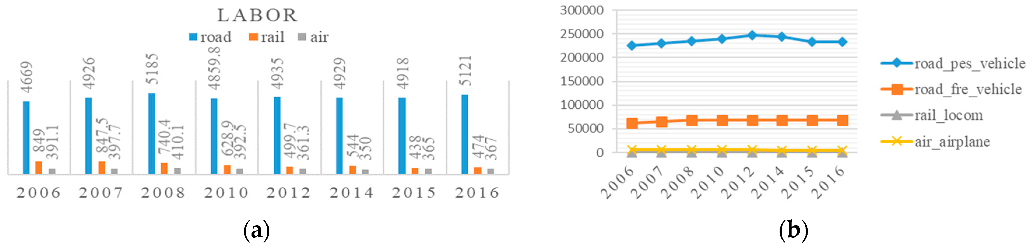
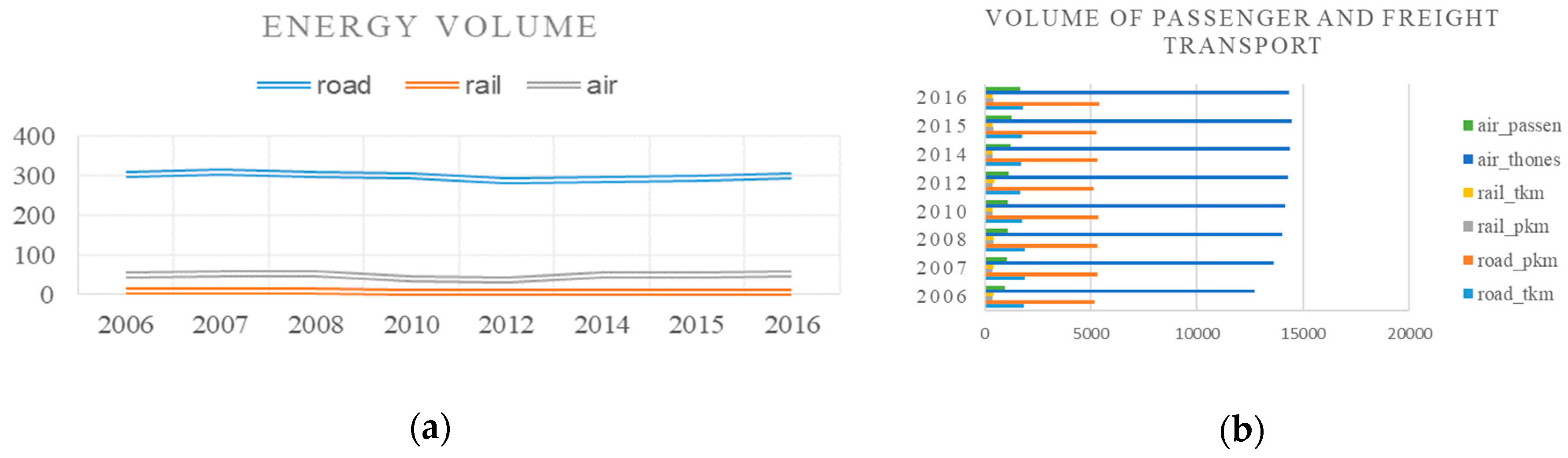
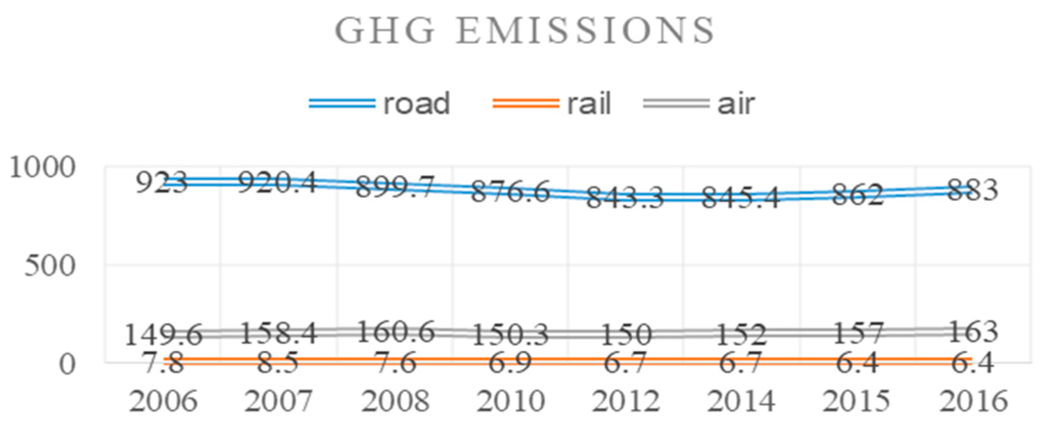
4.1. Analysis of Inputs and Outputs

Figure 1, where labor and number of assets for the road, rail and air transport sectors in European countries were shown, indicated that the road sector had a dominant number of employees, followed by the air and rail transport sectors. Within the road sector, the number of employees increased year by year with an insignificant decrease in 2010 and the largest number in 2008. In rail transport the number of employees continuously decreased until 2012, after that it started do slightly increase, while in air transport there was an increase from 2006 to 2008, an decrease from 2010 to 2014, when the number of employees was the lowest, after that it started again slightly to increase. These trends of road and air transport could be the result of the economic crisis. However, almost constant reduction of the number of employees in the rail and air transport sectors could be the consequence of the intensive improvement of economic efficiency, which does not include any measurement regarding employment (or unemployment). Regarding the number of assets, the leading sector was again the road sector, primarily in terms of passenger vehicles. The road sector showed steady growth of several assets, while the rail sector highlights continuously decrease. Several assets gradually increased after 2006 in the air sector and it were slightly reduced in 2012.

Trends of energy input, desirable outputs and undesirable output are shown in Figure 2a,b and Figure 3, respectively. The volume of energy consumption in the rail sector was the lowest as compared to the road and air sectors. Energy volume was reduced in road, rail and air after 2008 and started again to increase after 2012. Reasons for decreasing energy consumption could be found in the increase of oil prices and the strategy of de-carbonization. These reasons were especially notable in air transport which had more dominant freight transport as compared to passenger transport, even though both showed constant growth. Please note that the volume of both types of transport in air sector was expressed in thousand ton and millions of passengers. The volume of rail passenger and freight transport was increasing up to 2008, after which it continued to dominate and showed growth in 2012. However, passenger transport was reduced. The volume of freight and passenger transport in road transport was reduced in 2008, after which the volume of freight transport decreased, while the volume of passenger transport was constantly dominant, with a slight reduction in 2012. As for GHG emissions, gradual reduction in road, rail, and air until 2014 could be noted, probably due to technological advances in vehicles and sources of energy, as well as more stringent standards [23]. After 2014 in road and air transport the volume of GHG emissions started to increase, while in rail it remained unchanged.

4.2. Results of DEA Method

In this part of the paper, based on the objective of the study, the results of the application of the non-radial DEA model are presented. At this point, the potential factors of EEE are only mentioned, without any statistical or other analysis.

All DEA results were calculated by Excel Solver. The calculation was conducted for each transport sector separately and for each year. The availability of data was the best in terms of road transport sector, followed by air and rail.

The results for the road transport sector (

Table 5. Results of efficiency of non-radial DEA model and rank of TOPSIS method for the road sector (2006–2012).

Road Sector
DMUs	2006		2007		2008		2010		2012
	DEA	TOPSIS	DEA	TOPSIS	DEA	TOPSIS	DEA	TOPSIS	DEA	TOPSIS
	Non-Radial	Rank	Non-Radial	Rank	Non-Radial	Rank	Non-Radial	Rank	Non-Radial	Rank
BE	0.808649	17	0.929032	17	0.319853	19	0.769692	16	1	19
BG	0.546216	11	0.844309	8	0.357289	10	0.958431	9	1	7
CZ	0.637093	15	0.591504	16	0.631525	15	0.658219	18	0.612003	15
DK	1	13	1	14	0.343223	14	0.705374	13	0.91319	12
DE	1	26	1	25	0.444898	25	0.81077	25	1	28
EE	0.617846	5	0.622808	1	0.686869	6	0.708056	5	0.807294	5
IE	1	12	1	13	0.312296	13	1	12	1	14
EL	0.625318	20	0.717725	20	0.288885	20	0.81967	20	1	21
ES	0.564873	24	0.570622	24	0.607714	24	0.538116	23	0.742671	24
FR	0.86936	25	0.821412	26	0.325536	26	1	26	1	26
IT	1	27	1	27	0.289674	27	0.918007	27	0.997767	27
CY	0.419031	10	0.421868	10	0.17257	8	0.353261	8	0.493888	10
LV	0.780133	3	0.776361	5	0.741368	4	1	4	1	4
LT	1	1	1	3	1	2	1	2	1	1
LU	1	9	1	9	1	9	1	7	1	11
HU	0.550362	14	0.612014	12	0.623609	12	0.810149	10	0.941513	9
MT	0.747098	7	0.685189	7	0.091075	5	0.651429	6	0.669092	6
NL	0.605102	21	0.614736	21	0.511777	21	0.535244	21	0.681301	22
AT	0.43343	19	0.409689	19	0.398355	18	0.440404	19	0.490857	20
PL	0.769045	22	0.869976	22	0.697239	22	0.954807	22	0.993453	23
PT	0.560112	18	0.70439	15	0.446918	17	0.61483	17	0.792474	16
RO	1	6	1	4	0.808434	11	0.765552	14	0.78381	17
SI	1	4	1	6	0.753484	3	1	3	1	3
SK	1	2	1	2	1	1	1	1	1	2
FI	1	8	1	11	0.525652	7	0.887975	11	0.917381	13
SE	0.536462	16	0.605111	18	0.415428	16	0.875713	15	0.967949	18
UK	1	23	1	23	0.268397	23	0.878957	24	1	25
HR	/	/	/	/	/	/	/	/	0.744544	8

Green color: the best EEEI. Red color: the least EEEI.

and

Table 6. Results of efficiency of non-radial DEA model and rank of TOPSIS method for the road sector (2014–2016).

Road Sector
DMUs	2014		2015		2016
	DEA	TOPSIS	DEA	TOPSIS	DEA	TOPSIS
	Non-Radial	Rank	Non-Radial	Rank	Non-Radial	Rank
BE	1	22	1	24	1	23
BG	1	9	1	10	1	9
CZ	0.735	17	0.762	16	0.705	14
DK	0.705	11	0.705	13	0.709	11
DE	1	25	1	27	1	26
EE	0.841	15	0.918	17	0.867	16
IE	0.769	8	0.716	8	0.695	7
EL	1	7	1	4	1	3
ES	0.732	24	1	25	1	24
FR	1	27	0.932	28	0.948	28
IT	1	26	1	26	1	25
CY	0.549	14	0.523	12	0.475	13
LV	0.898	16	0.944	18	0.895	15
LT	1	2	1	2	1	1
LU	1	10	1	9	1	8
HU	0.924	12	0.879	14	0.854	12
MT	0.675	6	0.622	6	0.691	6
NL	1	23	1	22	1	20
AT	0.571	18	0.554	23	0.554	22
PL	1	20	1	15	1	17
PT	0.853	5	0.808	11	0.837	10
RO	0.813	21	0.901	20	0.906	19
SI	1	1	1	3	1	2
SK	1	4	1	7	1	4
FI	0.902	13	1	19	0.710	18
SE	0.995	19	0.929	21	0.990	21
UK	0.868	28	1	1	1	27
HR	0.768	3	0.721	5	0.698	5

Green color: the best EEEI. Red color: the least EEEI.

) indicated that the best EEEI for countries was in the green cells each year, meaning that these countries were relatively energy-environment efficient. The countries in red cells with the least EEEI were: Cyprus (CY) in 2006, 2008, 2010, 2012, 2014–2016, and Austria (AT) in 2007. Please note that EEEI was improved for both countries in 2012 and 2014 as compared to previous years, but after 2014 it slightly deteriorated. Regarding Cyprus (CY) it can be seen (see supplementary material) that in these years, all values of data for desirable variables were lower, while those for undesirable were higher in comparison with other DMUs. However, Austria (AT) was inefficient, probably due to a higher number of undesirable variables in comparison to other DMUs (see raw data in supplementary material). The improvement of EEE in the road sector could be a result of stricter policy measures through prioritization in de-carbonization with primary introduction of CO₂ emission standards for new passenger cars and heavy vehicles [1,50], highlighted the use of bioenergy and renewable energy [62], new technologies for vehicles and traffic management [1], as well as improved conditions of cabotage. The best value of EEEI for each year of the evaluation was for Lithuania (LT) and Luxemburg (LU), almost each year for Slovakia (SK) and Slovenia (SI) and thus they could be considered the countries with the best practices. The main reason lies in the fact that these countries had the lowest values for undesirable variables in comparison with other DMUs, while desirable variables were higher and comparable with other DMUs (see supplementary material). It could be also seen that most of the countries improved their EEEI in the period of 2014–2016, while Ireland (IE) worsened drastically the values of EEEI after 2012.

As far as the rail transport sector was concerned, the number of DMUs was smaller due to data unavailability (

Table 7. Results of efficiency of non-radial DEA model and rank of TOPSIS method for the rail sector (2006–2012).

Rail Sector
DMUs	2006		2007		2008		2010		2012
	DEA	TOPSIS	DEA	TOPSIS	DEA	TOPSIS	DEA	TOPSIS	DEA	TOPSIS
	Non-Radial	Rank	Non-Radial	Rank	Non-Radial	Rank	Non-Radial	Rank	Non-Radial	Rank
BE	0.771182	10	0.593661	9	0.716647	9	1	8	1	5
BG	0.490449	11	0.45795	8	0.309252	10	/	/	/	/
CZ	0.474833	16	0.467384	14	0.336824	13	0.391971	15	0.271762	10
DK	0.971713	8	0.899017	10	0.637045	11	0.413052	11	0.625863	8
DE	0.836313	19	0.857799	20	0.651819	19	0.653537	1	0.913981	15
EE	1	4	/	/	/	/	0.371963	13	/	/
IE	/	/	/	/	/	/	/	/	/	/
EL	0.170862	9	0.177281	11	0.158075	12	/	/	/	/
ES	0.666978	15	0.618655	16	0.454679	16	0.347673	17	0.528261	12
FR	1	18	1	19	1	18	0.948728	3	1	14
IT	1	17	1	17	1	14	1	4	/	/
CY	/	/	/	/	/	/	/	/	/	/
LV	1	6	1	4	1	3	1	6	1	4
LT	0.901956	5	0.984458	5	0.833261	5	0.712766	9	0.115761	7
LU	/	/	/	/	/	/	/	/	/	/
HU	1	12	0.57653	13	0.465083	7	0.323137	14	1	1
MT	/	/	/	/	/	/	/	/	/	/
NL	1	13	1	6	1	6	0.651163	10	0.963769	9
AT	0.951996	2	0.689355	2	0.563669	2	0.661709	7	0.879885	3
PL	1	16	0.933333	18	0.85144	17	0.777128	12	0.395634	11
PT	0.519374	7	0.670578	7	0.433445	8	/	/	/	/
RO	0.754073	14	0.394416	15	0.288133	15	0.329787	16	0.10985	13
SI	/	/	/	/	/	/	/	/	/	/
SK	/	/	0.830108	12	/	/	/	/	/	/
FI	0.980779	3	0.897204	3	0.705479	4	1	5	0.348291	6
SE	1	1	1	1	1	1	1	2	1	2
UK	0.593252	20	0.518208	21	0.382882	20	0.289564	18	0.607946	16
HR	/	/	/	/	/	/	/	/	/	/

Green color: the best EEEI. Red color: the least EEEI.

and

Table 8. Results of efficiency of non-radial DEA model and rank of TOPSIS method for the rail sector (2014–2016).

Rail Sector
DMUs	2014		2015		2016
	DEA	TOPSIS	DEA	TOPSIS	DEA	TOPSIS
	Non-Radial	Rank	Non-Radial	Rank	Non-Radial	Rank
BE	1	5	0.468	10	0.442	9
BG	/	/	0.221	16	/	/
CZ	0.335	11	0.418	9	0.439	8
DK	0.295	16	0.329	17	0.317	18
DE	1	19	1	20	1	20
EE	0.5	8	0.5	14	0.5	13
IE	0.5	17	0.5	18	0.5	16
EL	0.049	15	0.075	15	0.090	14
ES	1	6	0.620	4	1	6
FR	0.559	20	1	12	1	17
IT	1	2	1	6	1	4
CY	/	/	/	/	/	/
LV	1	9	1	7	1	7
LT	0.591	12	0.609	11	0.689	10
LU	/	/	/	/	/	/
HU	0.410	7	0.605	5	0.763	5
MT	/	/	/	/	/	/
NL	0.357	10	0.587	3	0.603	3
AT	1	1	1	1	1	1
PL	1	3	1	8	1	2
PT	/	/	/	/	/	/
RO	0.201	13	0.273	15	0.299	12
SI	/	/	/	/	/	/
SK	0.5	4	0.5	2	0.5	15
FI	0.623	18	0.633	19	0.762	19
SE	/	/	/	/	/	/
UK	0.291	21	0.351	21	0.358	21
HR	0.181	14	0.132	13	0.131	11

Green color: the best EEEI. Red color: the least EEEI.

). It could be noticed that the number of units with the highest value of EEEI was in 2006. The most efficient countries were represented in green cells per year. The least value of EEE Index in 2006, 2007, 2008, and period 2014–2016 was in a red cell for Greece (EL), due to lack of data, the second one for 2010 and 2012 were the United Kingdom (UK) and Romania (RO). However, similar to the case with road transport, inefficiency of these countries can be related to higher values of undesirable variables while desirable variables were lower in comparison with other DMUs (see supplementary material). It would be interesting to note that Latvia (LV), Italy (IT) and Sweden (SE) (data available only for 2006–2008, 2010, and 2012) had a constant best value of EEEI and represented the best practices. Based on the supplementary material, i.e., raw data, it can be seen that these countries had lower values for energy and GHG emissions while values for volume of passenger and freight transport were high in comparison with other DMUs. In terms of countries considered per each year, it could be concluded that scores of efficiency were not homogeneous. In 2012 half of DMUs were improved, while the other half of DMUs deteriorated. In the period 2014–2016 it could be noted drastically improvement of EEEI for Germany (DE), Austria (AT), and Poland (PL). In terms of the rail sector, the value of efficiency scores declined and a decline in efficiency for some countries could be attributed to insufficient market opening and modernization of rail sectors, incomplete implementation of modern traffic management systems such as ERTMS for European railway, insufficient European high speed rail network and interoperability, lack of modal shift in each country—i.e., involvement in the transport market [1,3]-as well as incomplete electrification of railway networks.

For the air transport sector, the availability of data was better than in the rail sector (

Table 9. Results of efficiency of non-radial DEA model and rank of TOPSIS method for the air sector (2006–2012).

Air Sector
DMUs	2006		2007		2008		2010		2012
	DEA	TOPSIS	DEA	TOPSIS	DEA	TOPSIS	DEA	TOPSIS	DEA	TOPSIS
	Non-Radial	Rank	Non-Radial	Rank	Non-Radial	Rank	Non-Radial	Rank	Non-Radial	Rank
BE	1	1	1	1	1	2	1	2	1	1
BG	/	/	0.706722	12	0.65753	10	0.821158	7	0.82482	11
CZ	0.980766	10	0.83411	9	0.827037	19	1	6	0.890042	6
DK	0.859713	14	0.69759	15	0.937466	3	0.897875	10	0.612392	14
DE	0.768173	19	0.642743	22	0.696089	23	1	19	0.751725	23
EE	/	/	0.71923	4	/	/	/	/	/	/
IE	1	12	1	14	0.829558	16	1	14	0.844267	19
EL	/	/	1	11	1	14	1	11	1	3
ES	1	18	0.946155	20	1	22	1	20	0.865467	21
FR	0.672936	20	0.625645	21	0.64646	24	0.580559	21	0.641927	24
IT	1	17	0.87757	19	0.924698	21	0.842596	18	0.878126	20
CY	1	3	1	5	1	4	1	3	1	7
LV	1	7	0.764706	7	0.888889	9	0.977778	5	0.923833	9
LT	0.729208	5	0.661475	6	1	7	/	/	0.842346	10
LU	1	2	1	2	1	1	1	1	1	2
HU	1	4	1	3	0.812856	8	1	4	1	4
MT	0.938662	6	/	/	1	5	/	/	0.703901	13
NL	1	16	1	18	1	20	1	17	1	15
AT	0.945716	13	0.833572	17	0.829785	17	0.916049	13	0.795946	16
PL	1	9	1	10	1	11	1	8	0.902043	8
PT	0.742749	15	0.629629	16	0.609771	18	0.647523	15	0.567826	17
RO	1	8	0.988549	8	0.844111	12	0.670554	9	/	/
SI	/	/	/	/	/	/	/	/	/	/
SK	/	/	/	/	1	6	/	/	/	/
FI	0.733084	11	0.566175	13	0.60486	15	0.609107	12	0.70449	5
SE	/	/	/	/	0.939663	13	0.869726	16	1	18
UK	0.648914	21	0.571663	23	0.574808	25	0.500327	22	1	22
HR	/	/	/	/	/	/	/	/	0.766475	12

Green color: the best EEEI. Red color: the least EEEI.

and

Table 10. Results of efficiency of non-radial DEA model and rank of TOPSIS method for the air sector (2014–2016).

Air Sector
DMUs	2014		2015		2016
	DEA	TOPSIS	DEA	TOPSIS	DEA	TOPSIS
	Non-Radial	Rank	Non-Radial	Rank	Non-Radial	Rank
BE	0.459	22	0.404	22	0.064	22
BG	0.759	13	0.621	11	1	3
CZ	0.843	6	0.757	7	0.225	6
DK	0.697	2	0.554	9	1	1
DE	1	26	1	26	1	26
EE	0.5	11	0.5	12	0.5	10
IE	0.299	23	0.267	23	0.196	23
EL	1	9	1	10	0.144	17
ES	0.821	25	0.761	25	0.147	25
FR	0.417	27	0.439	27	0.063	28
IT	0.932	20	0.928	18	0.229	18
CY	1	7	1	6	1	8
LV	0.680	8	0.541	14	0.217	15
LT	0.656	14	0.594	13	0.210	16
LU	1	1	1	1	1	2
HU	1	3	1	4	0.384	5
MT	0.436	17	0.531	19	0.200	19
NL	0.355	24	0.382	24	0.055	24
AT	0.443	18	0.307	20	0.254	20
PL	0.952	5	0.969	5	0.214	7
PT	0.506	21	0.499	21	0.148	21
RO	1	12	0.734	15	0.197	12
SI	0.324	15	0.332	17	0.346	14
SK	0.5	10	0.5	8	0.243	9
FI	0.633	19	0.605	2	0.219	4
SE	0.836	4	0.822	3	0.179	11
UK	1	28	1	28	1	27
HR	0.858	16	1	16	0.217	13

Green color: the best EEEI. Red color: the least EEEI.

), and the EEEI was also better compared to rail. The highest values of EEEI were for countries Cyprus (CY) and Luxembourg (LU). They had the best scores of efficiency throughout the entire evaluation period. Belgium (BE) and the Netherlands (NL) had the best value until 2012, after that their EEE indices drastically decreased. The lowest value of EEEI was in red cells for the United Kingdom (UK) in 2006, followed by Finland (FI) in 2007, the United Kingdom (UK) in 2008 and 2010, Portugal (PT) in 2012, Ireland (IE) in 2014 and 2015, and France (FR) in 2016. Similar to previous modes of transport, DMUs with higher values of desirable variables and lower values of undesirable variables (see supplementary material) in comparison with other DMUs have better values of EEEI. Surprisingly, the United Kingdom (UK) with three red values until 2012, had the best values for all three last years of evaluation period. The inefficiency of DMUs could be attributed to old aircraft, waiting for improvement of their aircraft’s fuel efficiency, or switching to green fuels [36].

Observing the highest values of EEEI for all transport sectors, Luxembourg (LU) was most frequently present in road and air transport sector, while data for the Luxembourg rail transport sector were missing. United Kingdom (UK) showed the lowest values of EEEI for rail and air transport sector.

4.3. Results of the TOPSIS Method

As with any other method, DEA also has its drawbacks. Regardless of its orientation, the DEA method has a tendency to assign maximum or minimum values to input and output, regardless of their initial values, by assigning the best value for EEEI. To eliminate this problem, weights of TOPSIS were used for considering the initial values of input and output variables. Furthermore, non-radial DEA shows discriminating power but does not indicate the difference between DMUs with efficiency results of 1. Consequently, a defect in the DEA analysis is the existence of multiple efficient units. In the literature, different DEA ranking methods exist for ranking DMUs that attempt to consider DMUs from input or output oriented aspects.

Therefore, the TOPSIS method with both viewpoints—i.e., pessimistic and optimistic-was used in order to evaluate and rank DMUs. Moreover, TOPSIS was employed with the aim of checking the results of the non-radial DEA model. Based on all these considerations, in order to verify differences between these two methods a research hypothesis was formed. The results of the TOPSIS method were calculated using Excel environment.

In terms of the road sector one country ranked first in three years, Lithuania (LT) in 2006, 2012 and 2016, while Slovakia (SK) ranked first in two years, 2008 and 2010. In 2007 the best ranked was Estonia (EE), in 2014 Slovenia (SI), and in 2015 United Kingdom (UK). In all cases, the EEEI was 1 (see Table 5 and Table 6).

In the rail sector, Sweden (SE) received a rank of 1 in 2006, 2007 and 2008, and Austria (AT) in 2014, 2015, and 2016. Germany (DE) and Hungary (HU) were ranked first in 2010 and 2012 (see Table 7 and Table 8). In all cases, except in the case of Germany (DE), the IEEE was 1.

As for air transport, Belgium (BE) was ranked 1 in 2006, 2007, and 2012, Luxembourg (LU) in 2008, 2010, 2014, and 2015, while Denmark (DK) received rank of 1 in 2016. In all cases the EEEI was 1. (see Table 9 and Table 10).

All the countries with a rank of 1 for the rail and air transport sectors (except the DE in 2010 for the rail sector) at the same time had the best value of EEEI. However, the results of TOPSIS method were different. For instance, for the road sector Lithuania (LT) was ranked 1 by TOPSIS in 2006, 2012 and 2016 and also had the best EEEI for those years, as well as Slovakia (SK) in 2008 and 2010, while in 2007 Estonia (EE) whose EEEI was 0.622 had a rank of 1.

In addition, the results of the TOPSIS method were different from the results of the non-radial DEA model. Estonia (EE), for example, had a rank of 1 in 2007 even though the result of the EEEI of the DEA model was lower: 0.622. Furthermore, considering other DMUs, we note similar situations. For the road sector in 2012, DMUs with ranks from 1 to 4 obtained from TOPSIS had efficiency scores of 1 obtained by the non-radial DEA model, while DMU with rank 5 had an efficiency score of 0.807. Moreover, for the same year Belgium (BE) with a rank of 19 by TOPSIS had an efficiency score 1 by the non-radial DEA method. The situation is similar for other years; for example, Luxembourg (LU) had an efficiency score of 1 for 2008 and Ireland for 2010, while with TOPSIS Luxembourg (LU) had 9 and Ireland (IE) 12. From 2014 to 2016 Belgium (BE) has EEEI equal 1, but it was ranked as 22, 24, and 23 respectively. The similar is for Bulgaria (BG), Germany (DE), Italy (IT), Luxemburg (LU), Netherlands (NL), and Poland (PL).

It is significant to note that the results of the TOPSIS method for the rail and air transport sectors were different for a large number of DMUs in comparison to the non-radial DEA model. For example, for rail Sweden (SE) was ranked first in 2006, 2007 and 2008, while in 2012 the best ranked was Hungary (HU); on the other side, both DMUs had the highest efficiency scores. However, in 2010 Germany (DE) was ranked first, although by the non-radial DEA model the obtained efficiency score was 0.653537. Germany (DE), Italy (IT), Latvia (LV), and Poland (PL) had the efficiency scores for 2014, 2015, and 2016 equal 1, while they were not ranked as first by TOPSIS.

Similar to the results of the TOPSIS for road, for rail France (FR) received an efficiency score of 1 in 2006 and 2008, yet was ranked 18; and for 2007 and 2012 it ranked 19 and 14 while having the highest efficiency score.

Regarding the air sector, the picture in terms of results given by DEA and TOPSIS is the same as with the road and rail sectors. Belgium (BE), with an efficiency score of 1 in 2006, 2007 and 2012 had a rank of 1, while in 2008 and 2010 Luxembourg (LU), with the highest efficiency score, ranked first. However, for example, Spain (ES), with an efficiency score of 1 by DEA model in 2006, 2008 and 2010 had ranks of 18, 22, and 20, while in 2007 the Netherlands (NL) ranked 18 with a 1 efficiency score, and in 2012 the United Kingdom (UK) ranked 22 yet had the highest efficiency score. Furthermore, Germany (DE) with the highest efficiency scores in 2014, 2015, and 2016 ranked 26.

Therefore, it could be said that the DEA is not the most suitable benchmarking tool in the field of the evaluation of the transport EEE.

Consequently, based on the significant differences between the results of the non-radial DEA model and the TOPSIS method, our research hypothesis could be confirmed. The reason for differences in results should be found in the fact that DEA considered inputs for a given level of outputs, while the TOPSIS method, in order to find the best DMUs, closest to the ideal positive solution and furthest from the negative weights its criteria. Another reason for differences in results of the TOPSIS method and the DEA method is the involvement of weights for each criterion, not only for variables in the goal function in the non-radial DEA model.

4.4. Discussion

Within Table 5 and Table 6, the results of non-radial DEA model and TOPSIS method for road sector were presented. Based on the results of non-radial DEA model efficient and non-efficient DMU can be seen. Considering the results of evaluation through the selected period, it can be seen that the lowest number of countries with the efficiency score of 1 was in 2008. Numerous DMUs are efficient, while one of them has the lowest score of efficiency. However, due to discrimination power of non-radial DEA model there is a little difference between non-efficient DMUs. In addition, it can be noticed that many countries obtained the efficiency score of 1 by DEA model, while only one was ranked as first with TOPSIS. In 2007, the country ranked as first by TOPSIS received relatively low efficiency score—i.e., only 7 countries were less efficient. However, considering the raw data (see supplementary material) the main reason for that is related to the TOPSIS method and values of raw data. For EE (Estonia) in 2007 the values of data are lower than that used as minimum criteria in TOPSIS and other data as maximum criteria for that country were sufficient in comparison with other alternatives. In general, the efficiency scores of more than three quarters of evaluated countries constantly increased after the 2012. Only one country was inefficient throughout the entire evaluation period by DEA, while it was ranked among first half of all countries by TOPSIS. The primarily reason for the difference between results of DEA and TOPSIS lies in the fact that TOPSIS evaluates countries with different criteria from two points of view. However, with the DEA method it is possible to change the efficiency of some DMUs if the raw data for them is changed. Based on that, some inefficient DMUs can become efficient and vice versa.

Considering the rail sector (Table 7 and Table 8) in comparison with road sector it can be seen that a significantly smaller number of countries have the highest efficiency. Within the rail sector, the most efficient countries were in 2006 and 2016. Regarding the application of TOPSIS method similar picture appears as in road sector. Beside the best efficiency score obtained with non-radial DEA model, some countries were near to the worst ranked by TOPSIS. Only one country had the efficiency score constantly very low throughout the entire evaluation period, and at the same time it was mostly ranked at the bottom of the list by TOPSIS.

Regarding the air sector (Table 9 and Table 10) it can be seen that the number of countries that obtained the highest efficiency score by DEA method was greater in comparison with rail and road sectors. However, such results were obtained due to the highest volume of transport realized by air sector with the lowest number of used assets. Furthermore, the level of consumed energy and produced emissions were lower in comparison with road sector.

5. Conclusions

Over the last decade, the main and intensive topics of research among scholars were energy consumption and environmental impacts caused by transport systems. One of the major contributors to energy consumption and endangerment of the environment in Europe has been the overall transport sector. Among all modes of transport, the road sector was recognized as the main energy consumer and environmental pollutant. Notwithstanding the importance of this fact, there was not any research on energy-environment efficiency of European transport sectors.

In this paper, therefore energy-environment efficiency (EEE) of European road, rail and air transport sectors were evaluated using a modified non-radial DEA model under the joint production framework proposed by Wu et al. [6]. The evaluation was conducted for European countries in terms of road, rail and air transport sectors for the period 2006 to 2008, 2010, 2012, 2014, 2015, and 2016. The first reason for the adoption of non-radial DEA model was simultaneous minimization of energy inputs and undesirable outputs for the given level of inputs and outputs, and this was a primary motivation for our paper. This non-radial DEA model has benefits in terms of the ability to use different non-proportional adjustments and weighting for energy inputs and undesirable outputs. In the paper, non-energy inputs, named several assets (see Table 3), were defined and used in the evaluation of transport EEE for the first time.

Furthermore, the concept of transport EEE was introduced in this study through the reflection of the relationship among transport energy, non-energy inputs, and transport desirable and undesirable outputs. Following the aims of the paper, all used variables were described and their changes were presented only through figures-without any statistical analysis, while factors of EEE were only mentioned.

An additional contribution provided in the paper was the introduction of the TOPSIS method as a tool in the evaluation of transport EEE through the ranking of DMUs. With this evaluation of EEE for European road, rail, and air transport sectors, the stakeholders from each member state may find the best practices toward the most efficient means of improving overall efficiency.

Based on the results of the DEA approach, we found that the lowest number of DMUs with the best value of EEEI for the road sector was in 2008. In terms of rail transport, the highest DMUs had the best EEEI in 2006, and after a decrease in 2007, has since remained fairly unchanged. As far as air transport was concerned, the best value of EEEI was attributed to the least number of DMUs in 2007 and 2012.

Rail and air transport had much more room for EEE improvement than the road transport sector, which was relatively efficient in many European countries. Accordingly, it could be concluded that periodical documents of EU policies for sustainable transport contributed to the improvement of EEE in road transport sector. However, a modal shift as one of the policies and advanced technologies was not fully completed for rail transport. Therefore, the potential of the rail transport sector was not totally realized, which resulted in inefficiency within the rail transport sector. Ramanathan’s [11] findings confirmed this, stating that rail transport could capture around 50% of the expected traffic, which would result in saving of about 37% in energy consumption and associated CO₂ emissions that would result if the existing patterns of modal split did not change. Additionally, Song et al. [22] stated that a higher rate of railway concentration was associated with higher environment efficiency. In terms of air transport, the measures for EEE improvement implied newer and more fuel-efficient aircraft through new technology and larger planes [36].

The main conclusions could be drawn through the application of the TOPSIS method. All DMU with EEEI result 1 had the first rank. However, in some cases DMUs with an EEEI score 1 and lower had a rather wildly varying ranks. This is because the non-radial DEA model minimizes desirable and undesirable inputs for a given level of the desirable outputs. Then, the non-radial model benchmarks one DMU in comparison with others DMUs. However, based on the changes of raw data (see supplementary material) with the non-radial DEA model some inefficient DMUs can become efficient and vice versa. Then, the consequence could be a result of the TOPSIS method considering all inputs and outputs with the possibility of minimization and maximization during the process of analysis–they strove for clear values. Furthermore, the weights used in the TOPSIS method were assigned to each input and output.

The authors proposed using the TOPSIS method for finding the best practice in accordance with the challenges of European transport. The main European challenge is the demand for transport, which has significantly increased since 2000 and is expected to continue growing. On the other hand, the European transport sector is heavily dependent on oil. It releases GHGs and air pollutants into the atmosphere and contributes to climate change, but also makes the European economy more vulnerable regarding fluctuations in global energy supplies and prices [69]. The overall improvement of transport EEE in Europe could be achieved through progress in terms of EEE for each member state for each transport sector.

Bearing that in mind, finding the best practice which realizes the highest volume of freight and passenger transport with minimal energy consumption and environmental impact could be found through the TOPSIS method rather than any DEA approach.

Consequently, the authors highlight the importance of including of the TOPSIS method in future evaluation of transport EEE. Some proposals for the development of the European transport sector in terms of energy-environment efficiency are:

• Intensifying efforts in the implementation policy of modal shift from road and air transport sectors to eco-friendly sectors, such as rail transport, primarily in developed countries, in order to increase total EEE.
• Strengthening transport infrastructure and infrastructure components in terms of rail transport at bottlenecks, as well as total modernization of rail transport sectors.
• Reinforcing the adoption of technological innovations and standards in each transport sector.
• Employment of alternative sources of energy and modes of transport that have a potential to reduce energy consumption and environment impacts.

As for future work, the focus should be on research in terms of changes in results of non-radial DEA models with weights assigned to all inputs and outputs, as compared to the TOPSIS method. Additionally, TOPSIS could be used with other DEA models for checking results during the evaluation of transport EEE. Moreover, attention should be drawn to research into the impacts of technological innovation for improving transport EEE, primarily in the rail transport sector.

References

1. European Commission. A European Strategy for Low-Emission Mobility-COM (2016) 501 Final; European Commission: Brussels, Belgium, 2016. [Google Scholar]
2. European Environmental Agency. Final Energy Consumption by Sector and Fuel; European Environmental Agency: Brussels, Belgium, 2015. [Google Scholar]
3. European Commission. White Paper on transport—Roadmap to a Single European Transport Area—Towards a Competitive and Resource-Efficient Transport System; European Commission: Brussels, Belgium, 2011. [Google Scholar]
4. Zhou, P.; Ang, B.W.; Poh, K.L. A survey of data envelopment analysis in energy and environmental studies. Eur. J. Oper. Res. 2008, 189, 1–18. [Google Scholar] [CrossRef]
5. Meng, F.Y.; Su, B.; Thomson, E.; Zhou, D.Q.; Zhou, P. Measuring China’s regional energy and carbon emission efficiency with DEA models: A survey. Appl. Energy 2016, 183, 1–21. [Google Scholar] [CrossRef]
6. Wu, J.; Zhu, Q.; Yin, P.; Song, M. Measuring energy and environmental performance for regions in China by using DEA-based Malmquist indices. Oper. Res. Int. J. 2015, 17, 715–735. [Google Scholar] [CrossRef]
7. Wang, B.; Nistor, I.; Murty, T.; Wei, Y.M. Efficiency assessment of hydroelectric power plants in Canada: A multi criteria decision making approach. Energy Econ. 2014, 46, 112–121. [Google Scholar] [CrossRef]
8. Zhou, G.H.; Chung, W.; Zhang, Y.X. Measuring energy efficiency performance of China’s transport sector: A data envelopment analysis approach. Expert Syst. Appl. 2014, 41, 709–722. [Google Scholar] [CrossRef]
9. Zhou, P.; Ang, B.W. Linear programming models for measuring economy-wide energy efficiency performance. Energy Policy 2008, 36, 2911–2916. [Google Scholar] [CrossRef]
10. Ramanathan, R. A holistic approach to compare energy efficiencies of different transport modes. Energy Policy 2000, 28, 743–747. [Google Scholar] [CrossRef]
11. Ramanathan, R. Estimating energy consumption of transport modes in India using DEA and application to energy and environmental policy. J. Oper. Res. Soc. 2005, 56, 732–737. [Google Scholar] [CrossRef]
12. Leal, I.C.; de Almada Garcia, P.A.; de Almeida D’Agosto, M. A data envelopment analysis approach to choose transport modes based on eco-efficiency. Environ. Dev. Sustain. 2012, 14, 767–781. [Google Scholar] [CrossRef]
13. Lin, W.B.; Chen, B.; Xie, L.N.; Pan, H.R. Estimating Energy Consumption of Transport Modes in China Using DEA. Sustainability 2015, 7, 4225–4239. [Google Scholar] [CrossRef] [Green Version]
14. Cui, Q.; Li, Y. An empirical study on the influencing factors of transportation carbon efficiency: Evidences from fifteen countries. Appl. Energy 2015, 141, 209–217. [Google Scholar] [CrossRef]
15. Cui, Q.; Li, Y. The evaluation of transportation energy efficiency: An application of three-stage virtual frontier DEA. Transp. Res. Part D Transp. Environ. 2014, 29, 1–11. [Google Scholar] [CrossRef]
16. Liu, X.H.; Wu, J. Energy and environmental efficiency analysis of China’s regional transportation sectors: A slack-based DEA approach. Energy Syst. Optim. Model. Simul. Econ. Asp. 2017, 8, 747–759. [Google Scholar] [CrossRef]
17. Chang, Y.T.; Park, H.S.; Jeong, J.B.; Lee, J.W. Evaluating economic and environmental efficiency of global airlines: A SBM-DEA approach. Transp. Res. Part D Transp. Environ. 2014, 27, 46–50. [Google Scholar] [CrossRef]
18. Chang, Y.T.; Zhang, N.; Danao, D.; Zhang, N. Environmental efficiency analysis of transportation system in China: A non-radial DEA approach. Energy Policy 2013, 58, 277–283. [Google Scholar] [CrossRef]
19. Park, Y.S.; Lim, S.H.; Egilmez, G.; Szmerekovsky, J. Environmental efficiency assessment of US transport sector: A slack-based data envelopment analysis approach. Transp. Res. Part D Transp. Environ. 2018, 61, 152–164. [Google Scholar] [CrossRef]
20. Chang, Y.T. Environmental efficiency of ports: A Data Envelopment Analysis approach. Marit. Policy Manag. 2013, 40, 467–478. [Google Scholar] [CrossRef]
21. Liu, Z.; Qin, C.X.; Zhang, Y.J. The energy-environment efficiency of road and railway sectors in China: Evidence from the provincial level. Ecol. Indic. 2016, 69, 559–570. [Google Scholar] [CrossRef]
22. Song, M.L.; Zhang, G.J.; Zeng, W.X.; Liu, J.H.; Fang, K.N. Railway transportation and environmental efficiency in China. Transp. Res. Part D Transp. Environ. 2016, 48, 488–498. [Google Scholar] [CrossRef]
23. Beltran-Esteve, M.; Picazo-Tadeo, A.J. Assessing environmental performance trends in the transport industry: Eco-innovation or catching-up? Energy Econ. 2015, 51, 570–580. [Google Scholar] [CrossRef]
24. Egilmez, G.; Park, Y.S. Transportation related carbon, energy and water footprint analysis of US manufacturing: An eco-efficiency assessment. Transp. Res. Part D Transp. Environ. 2014, 32, 143–159. [Google Scholar] [CrossRef]
25. Cui, Q.; Li, Y. Evaluating energy efficiency for airlines: An application of VFB-DEA. J. Air Transp. Manag. 2015, 44–45, 34–41. [Google Scholar] [CrossRef]
26. Chen, X.H.; Gao, Y.Y.; An, Q.X.; Wang, Z.R.; Neralic, L. Energy efficiency measurement of Chinese Yangtze River Delta’s cities transportation: A DEAwindow analysis approach. Energy Effic. 2018, 11, 1941–1953. [Google Scholar] [CrossRef]
27. Feng, C.; Wang, M. Analysis of energy efficiency in China’s transportation sector. Renew. Sustain. Energy Rev. 2018, 94, 565–575. [Google Scholar] [CrossRef]
28. Omrani, H.; Shafaat, K.; Alizadeh, A. Integrated data envelopment analysis and cooperative game for evaluating energy efficiency of transportation sector: A case of Iran. Ann. Oper. Res. 2019, 274, 471–499. [Google Scholar] [CrossRef]
29. Makridou, G.; Andriosopoulos, K.; Doumpos, M.; Zopounidis, C. Measuring the efficiency of energy-intensive industries across European countries. Energy Policy 2016, 88, 573–583. [Google Scholar] [CrossRef]
30. Hu, J.L.; Honma, S. A Comparative Study of Energy Efficiency of OECD Countries: An Application of the Stochastic Frontier Analysis. Energy Procedia 2014, 61, 2280–2283. [Google Scholar] [CrossRef] [Green Version]
31. Song, M.L.; Zheng, W.P.; Wang, Z.Y. Environmental efficiency and energy consumption of highway transportation systems in China. Int. J. Prod. Econ. 2016, 181, 441–449. [Google Scholar] [CrossRef]
32. Chang, Y.T.; Zhang, N. Environmental efficiency of transportation sectors in China and Korea. Marit. Econ. Logist. 2017, 19, 68–93. [Google Scholar] [CrossRef]
33. Chu, J.-F.; Wu, J.; Song, M.-L. An SBM-DEA model with parallel computing design for environmental efficiency evaluation in the big data context: A transportation system application. Ann. Oper. Res. 2018, 270, 105–124. [Google Scholar] [CrossRef]
34. Cui, Q.; Li, Y. Airline energy efficiency measures considering carbon abatement: A new strategic framework. Transp. Res. Part D Transp. Environ. 2016, 49, 246–258. [Google Scholar] [CrossRef]
35. Li, Y.; Wang, Y.Z.; Cui, Q. Energy efficiency measures for airlines: An application of virtual frontier dynamic range adjusted measure. J. Renew. Sustain. Energy 2016, 8, 015901. [Google Scholar] [CrossRef]
36. Arjomandi, A.; Seufert, J.H. An evaluation of the world’s major airlines’ technical and environmental performance. Econ. Model. 2014, 41, 133–144. [Google Scholar] [CrossRef]
37. Cui, Q.; Wei, Y.M.; Li, Y. Exploring the impacts of the EU ETS emission limits on airline performance via the Dynamic Environmental DEA approach. Appl. Energy 2016, 183, 984–994. [Google Scholar] [CrossRef]
38. Cui, Q.; Li, Y.; Yu, C.L.; Wei, T.M. Evaluating energy efficiency for airlines: An application of Virtual Frontier Dynamic Slacks Based Measure. Energy 2016, 113, 1231–1240. [Google Scholar] [CrossRef]
39. Li, Y.; Wang, Y.Z.; Cui, Q. Has airline efficiency affected by the inclusion of aviation into European Union Emission Trading Scheme? Evidences from 22 airlines during 2008–2012. Energy 2016, 96, 8–22. [Google Scholar] [CrossRef]
40. Montanari, R. Environmental efficiency analysis for enel thermo-power plants. J. Clean. Prod. 2004, 12, 403–414. [Google Scholar] [CrossRef]
41. Ouattara, A.; Pibouleau, L.; Azzaro-Pantel, C.; Domenech, S.; Baudet, P.; Yao, B. Economic and environmental strategies for process design. Comput. Chem. Eng. 2012, 36, 174–188. [Google Scholar] [CrossRef] [Green Version]
42. Wang, Y.; Chen, Y.; Benitez-Amado, J. How information technology influences environmental performance: Empirical evidence from China. Int. J. Inf. Manag. 2015, 35, 160–170. [Google Scholar] [CrossRef]
43. Delgarm, N.; Sajadi, B.; Delgarm, S. Multi-objective optimization of building energy performance and indoor thermal comfort: A new method using artificial bee colony (ABC). Energy Build. 2016, 131, 42–53. [Google Scholar] [CrossRef]
44. Ziemele, J.; Pakere, I.; Blumberga, D. The future competitiveness of the non-Emissions Trading Scheme district heating systems in the Baltic States. Appl. Energy 2016, 162, 1579–1585. [Google Scholar] [CrossRef]
45. Babazadeh, R.; Razmi, J.; Rabbani, M.; Pishvaee, M.S. An integrated data envelopment analysise mathematical programming approach to strategic biodiesel supply chain network design problem. J. Clean. Prod. 2017, 147, 694–707. [Google Scholar] [CrossRef]
46. Sueyoshi, T.; Goto, M. Returns to Scale and Damages to Scale with Strong Complementary Slackness Conditions in DEA Assessment: Japanese Corporate Effort on Environment Protection. Energy Econ. 2012, 34, 1422–1434. [Google Scholar] [CrossRef]
47. Choi, Y.; Zhang, N.; Zhou, P. Efficiency and abatement costs of energy-related CO2 emissions in China: A slacks-based efficiency measure. Appl. Energy 2012, 98, 198–208. [Google Scholar] [CrossRef]
48. Yaqubi, M.; Shahraki, J.; Sabouni, M.S. On dealing with the pollution costs in agriculture: A case study of paddy fields. Sci. Total Environ. 2016, 556, 310–318. [Google Scholar] [CrossRef]
49. Charnes, A.; Cooper, W.W.; Rhodes, E. Measuring the efficiency of decision making units. Eur. J. Oper. Res. 1978, 2, 15. [Google Scholar] [CrossRef]
50. Voltes-Dorta, A.; Perdiguero, J.; Jimenez, J.L. Are car manufacturers on the way to reduce CO2 emissions? A DEA approach. Energy Econ. 2013, 38, 77–86. [Google Scholar] [CrossRef]
51. Banker, R.D.; Charnes, A.; Cooper, W.W. Some Models for Estimating Technical and Scale Inefficiencies in Data Envelopment Analysis. Manag. Sci. 1984, 30, 1078–1092. [Google Scholar] [CrossRef] [Green Version]
52. Bian, Y.W.; Yang, F. Resource and environment efficiency analysis of provinces in China: A DEA approach based on Shannon’s entropy. Energy Policy 2010, 38, 1909–1917. [Google Scholar] [CrossRef]
53. Wang, J.-M.; Sun, Y.-F. The Application of Multi-Level Fuzzy Comprehensive Evaluation Method in Technical and Economic Evaluation of Distribution Network. In Proceedings of the 2010 International Conference on Management and Service Science (MASS), Wuhan, China, 24–26 August 2010; pp. 1–4. [Google Scholar]
54. Hwang, C.-L.; Yoon, K. Multiple Attribute Decision Making: Methods and Applications—A State-of-the-Art Survey; Springer: Berlin, Germany, 1981. [Google Scholar]
55. Behzadian, M.; Otaghsara, S.K.; Yazdani, M.; Ignatius, J. A state-of the-art survey of TOPSIS applications. Expert Syst. Appl. 2012, 39, 13051–13069. [Google Scholar] [CrossRef]
56. Hosseinzadeh Lotfi, F.; Fallahnejad, R.; Navidi, N. Ranking Efficient Units in DEA by Using TOPSIS Method. Appl. Math. Sci. 2011, 5, 10. [Google Scholar]
57. Jahantigh, M.; Hosseinzadeh Lotfi, F.; Moghaddas, Z. TRanking of DMUs by using TOPSIS and different ranking models in DEA. Int. J. Ind. Math. 2013, 5, 9. [Google Scholar]
58. European Union. EU Energy and Transport in Figures—Statistical Pocketbook 2009; Publications Office of the European Union: Luxembourg, 2009. [Google Scholar]
59. European Union. EU Energy and Transport in Figures—Statistical Packetbook 2010; Publications Office of the European Union: Luxembourg, 2010. [Google Scholar]
60. European Union. EU Transport in Figures—Statistical Pocketbook 2011; Publications Office of the European Union: Luxembourg, 2011. [Google Scholar]
61. European Union. EU Transport in Figures—Statistical Pocketbook 2012; Publications Office of the European Union: Luxembourg, 2012. [Google Scholar]
62. European Environmental Agency. Towards a Green Economy in Europe—EU Environmental Policy Targets and Objectives 2010–2050; Publications Office of the European Union: Luxembourg, 2013. [Google Scholar]
63. European Union. EU Transport in Figures—Statistical Pocketbook 2014; Publications Office of the European Union: Luxembourg, 2014. [Google Scholar]
64. European Union. EU Transport in Figures—Statistical Pocketbook 2015; Publications Office of the European Union: Luxembourg, 2015. [Google Scholar]
65. European Union. EU Transport in Figures—Statistical Pocketbook 2016; Publications Office of the European Union: Luxembourg, 2016. [Google Scholar]
66. European Union. EU Transport in Figures—Statistical Pocketbook 2017; Publications Office of the European Union: Luxembourg, 2017. [Google Scholar]
67. European Union. EU Transport in Figures—Statistical Pocketbook 2018; Publications Office of the European Union: Luxembourg, 2018. [Google Scholar]
68. Nakanishi, Y.J.; Falcocchio, J.C. Performance assessment of intelligent transportation systems using data envelopment analysis. Res. Transp. Econ. 2004, 8, 181–197. [Google Scholar] [CrossRef]
69. European Environmental Agency. Towards Clean and Smart Mobility—Transport and Environment in Europe; Publications Office of the European Union: Luxembourg, 2016. [Google Scholar]
Figure 1. Trends of non-energy inputs for labor (a) and (b) number of assets.
Energies 12 02907 g001
Figure 2. Trends of energy input (a), desirable outputs (b).
Energies 12 02907 g002
Figure 3. Undesirable output.
Energies 12 02907 g003