Non-Intrusive Load Monitoring System Based on Convolution Neural Network and Adaptive Linear Programming Boosting

Abstract

Non–intrusive load monitoring based on power measurements is a promising topic of appliance identification in the research of smart grid; where the key is to avoid the power sub-item measurement in load monitoring. In this paper; a three–step non–intrusive load monitoring system (TNILM) is proposed. Firstly; a one dimension convolution neural network (CNN) is constructed based on the structure of GoogLeNet with 2D convolution; which can zoom in on the differences in features between the different appliances; and then effectively extract various transient features of appliances. Secondly; comparing with various classifiers; the Linear Programming boosting with adaptive weights and thresholds (ALPBoost) is proposed and applied to recognize single–appliance and multiple–appliance. Thirdly; an update process is adopted to adjust and balance the parameters between the one dimension CNN and ALPBoost on–line. The TNILM is tested on a real–world power consumption dataset; which comprises single or multiple appliances potentially operated simultaneously. The experiment result shows the effectiveness of the proposed method in both identification rates.

1. Introduction

As the most widely used energy by human beings, there is a great demand of electricity in the world and improving the efficiency of electrical energy can properly mitigate the gradual deterioration of the global environment [1]. With the rise of artificial intelligence, the smart grid has become an important direction for the development of the smart home, for which the key is mainly embodied in advanced metering infrastructures (AMI) [2,3].

As one of the important components of AMI, load monitoring is the first step for the implementation of the smart grid. Current meters can only record the total amount of electricity, which contains limited load information and cannot accurately analyze the customers’ internal load components [4]. Thus, this must be overcome to support the two–direction interactive services and smart power services. Traditional methods mainly adopt intrusive load monitoring (ILM), in which the sensors are installed on the customers’ appliances to measure the electric voltage and current waveforms. The advantage of ILM is that the monitoring data is accurate and reliable, while it has some drawbacks such as the poor practical operation, high cost, and low acceptance by customers.

The idea of non–intrusive load monitoring (NILM) was put forward by Hart in the 1980s [5]. NILM could be roughly divided into transient and steady–state strategies, both with the requirement of substantial measurement points of current, voltage, etc. [6] which are relatively stable, namely load signatures (LS). By collecting and analyzing the LS of appliances, the working state of the appliances could be monitored. The essence of NLIM is the load decomposition, which means that the total load information of customers is decomposed into the information of various single appliances. Therefore, we could obtain the customers’ information, including their energy consumption and state of the appliance. Compared with intrusive load monitoring, the power analysis based on NILM technology is simple, economical, and reliable, which is more acceptable for residences [3,5,7]. Meanwhile, smart homes and smart grids have flourished in recent years. Therefore, NILM has attracted widespread attention since its proposal. Various NILM systems have been proposed based on mathematical optimization [8,9,10,11] and machine learning [12,13,14,15,16,17,18,19,20,21,22,23,24,25,26]. The details of some proposed systems will be discussed in Section 2.

As shown in Figure 1, an innovative three–step Non–Intrusive Load Monitoring (TNILM) system is proposed. In Figure 1, the proposed TNILM system is described. Our proposed NILM apparatus is installed at the electricity service entry of consumers. The system utilizes load transient response features captured by the TNILM system. In recent years, as an efficient recognition method, the convolutional neural network has attracted widespread attention. According to the structure of GoogLeNet [27], the novel 1D convolution neural network (1D–CNN) has been constructed to draw transient features from current appliances for the subsequent identification. As a semi–supervised classifier, Linear Programming Boost (LPBoost) maximizes the margin between training samples of different classes, which is especially suited for applications of joint classification and feature selection in structured domains [28]. Thus, in order to enhance the effectiveness of the classifiers in load monitoring, adaptive Linear Programming Boosting (ALPBoost) classifiers are implemented to recognize appliances by the transient features. For better accuracy of load monitoring, a novel loss function based on the L2 regulation term is applied to adjust the parameters of 1D–CNN and ALPBoost, which is mainly applied in the third step of the system as an updated discriminant process.

This paper is organized as follows: The existing NILM systems are surveyed in Section 2. The details of the proposed TNILM system are presented in Section 3, including the three main steps. The experiments are described in Section 4.

2. Related Work

Several NILM systems have been studied, which could roughly be divided into two categories. One is the method applying mathematical optimization [8,10,11,13,29], and the other one is based on pattern recognition [14,15,16,17,18,19,20,21,22,23,24,25,30].

In 2012, Parson et al. [31] proposed an approach in which prior models of general appliance types are tuned to specific appliance instances using only signatures extracted from the aggregate load. The method is applied in an iterative manner until all appliances for which prior behavior models are known were disaggregated. In 2014, Lin et al. [13] proposed an improved time–frequency analysis–based NILM system, which is composed of three components, including data acquisition, transient feature extraction, and load identification. In [32], to further improve the accuracy of the load monitoring, they proposed a system which incorporates a multi–resolution S–transform with the ant colony algorithm to develop the load identification, transforming into a modified 0–1 multidimensional knapsack problem.

In 2015, Ahmadi et al. [29] first merged the loads’ current and voltage waveforms into a comprehensive library. Then they found that each load of the appliance is similar to the Face recognition [33]. Thus, a face recognition algorithm was employed in their system. The paper shows that by feature combinations, the systems smart meters could be accessed at any time when the library is stored.

In addition, we have surveyed the NILM systems based on pattern recognition. In [14,15,30], the authors combined the k–Nearest Neighbor (KNN) algorithm with other algorithms to load monitoring, given the transient feature of a single appliance. Tsai et al. [34] proposed an adaptive non–intrusive appliance load monitoring (ANIALM) system which utilizes the transient features to track the energy consumption of each appliance. In the system, KNN, back–propagation (BP), and neural network with artificial immune algorithm (AIA) [35] is applied to identify different types of appliances and detect the operation status of the appliance. From the experimental results of different actual environments, the accuracy of the system reached was above 90%. Saitoh et al. [14] applied the improved KNN and support vector machines (SVM) algorithms to recognize the appliances and detect the states of the appliances according to the ten transient features of the current.

In [9,15,16,17,18], a neural network is employed by NILM. Srinivasan D proposed a neural–network (NN)–based approach to make the nonintrusive harmonic source identification. By comparing multilayer perceptron (MLP), radial basis function (RBF) network, and linear support vector machines (LSVM) with RBF kernels, the results show that the Multi-Layer Perceptron (MLP) are the best signature identification methods. Chang et al. [16] combined artificial neural networks with turn–on transient energy analysis to improve recognition accuracy and computational speed. In [9], the authors applied the power spectrum of the wavelet transform coefficients (WTCs) in different scales calculated by Parseval’s theorem and the BP neural network to achieve the appliance identification.

In [19,20,21,22], the machine learning algorithms involving SVM and AdaBoost are presented based on the steady–state or the transient characteristics extracted from the appliances. These methods could effectively deal with the identification of some common home appliances. With this method, the accuracy is relatively high, when a load of the appliance is in a single state.

The aforementioned methods are mainly pattern recognition methods based on supervised learning [23]. Moreover, there are some other methods for NILM based on unsupervised learning.

The NILM systems [24,25,26,29,35,36] based on unsupervised learning could effectively weaken the impact of the tag data of the appliances, which means that the manual intervention could be reduced and the utility could be enhanced. These methods generate the appliances’ type through the steady–state characteristics of the monitoring data to screen out the status of the appliances.

In [26], Kim studied the distribution of the working process of the electricity–consuming equipment; the factorial hidden Markov model is applied to simplify the complicated process of labeling the appliances. However, when a large number of different appliances are running simultaneously, the recognition accuracy is limited, and this method is easy to fall into the local optimum.

To deal with the identification scenarios of higher complexity, some improved or comprehensive pattern recognition algorithms are designed. For example, in [37], a NILM system integrating Fuzzy C–Means clustering–piloting Particle Swarm Optimization with Neuro–Fuzzy Classification is proposed, which shows that the Fuzzy Logic theory could effectively handle the hybrid load identification. The literature [38] adopted the self–organizing map (SSOM)/Bayesian identifier for load monitoring, and the Bayesian identifier could provide the probability of the unknown load belonging to each specific type of load, which overcomes the disadvantages of the usual absolute decision–making methods, but this method fails to consider the load classification with multi–state transfer. Kolter et al. [24,39] apply the Factorial Hidden Markov Model (FHMM) technique and discriminative sparse coding to energy disaggregation. As a dynamic pattern recognition tool, FHMM can effectively model, classify, and sequence analysis through load monitoring information over time spans when there are few types of appliances.

Guo Z et al. [40] presented a model, named Explicit–Duration Hidden Markov Model with differential observations (EDHMM–diff) to detect and estimate the status of individual household appliances through the signal of the total monitoring load, and solve the overlapping phenomenon of the active signals, which are between the target electric appliance and other electrical equipment. Wang Z et al. [41] integrated mean–shift clustering with multidimensional linear discriminates based on unsupervised learning. Actual results revealed the performance of the system on load monitoring. However, the accuracy is relatively low compared with the nonintrusive load detection systems based on supervised learning. In summary, the load identification algorithms based on supervised learning emerge in an endless stream, but the types of loads involved are few, and the processing scenarios are relatively simple. The performance under complex scenarios needs further research. Compared with the algorithms based on supervised learning, the recognition algorithms based on unsupervised learning, although they are not accurate at present, have the advantage of reducing manual intervention and have good prospects for development [4]. We have listed the characteristics of some of the references in

Table 1. Comparison of the load identification algorithms.

Method Category		Algorithm Category	Application Scenario	Accuracy
mathematical optimization		Factorial Hidden Markov Models [10,24,26,39]	household appliances	70–95%
		0–1 multidimensional knapsack algorithm [13]	Several common household appliances	85–90%
pattern recognition	supervised learning	KNN [14,15,33]	Common household appliances	78–100%
		Neural Network [9,15,16,17,18,35]		70–100%
		SVM or AdaBoost [19,20,21,22]		85–99%
	unsupervised learning	Hidden Markov Models [24,26,39,40]	Several common household appliances	52–98%
		self–organizing map (SSOM)/Bayesian [38]; Fuzzy C–Means clustering [37]; integrate mean–shift clustering [41];		70–85.5%

Note: The experimental accuracy of some of the literature is obtained by reading a large amount of papers and then extracting it. The experimental accuracy of some other papers is obtained through the literatures’ experiments and our verification, and all experiments utilize the steady or transient features in load monitoring.

.

3. Three–Step Non–Intrusive Load Monitoring System

For the NILM, the key is to extract features of different appliances for load monitoring and decomposition. Generally, we can get the transient data of the active appliances from the outdoor meters such as the current, voltage, and harmonic wave signal, etc. The data could be regarded as the “photo” of the user status of a customer’s appliances, from which we need to distinguish the individuals by feature extraction. In most cases, the information of current, voltage, and other measured data can all be applied to help analyze the characteristics, but in this paper, for the sake of convenience, we only use the transient data of the current, which will not influence the results much [1,4]. Above all, based on the ideas aforementioned, we proposed a three–step non–intrusive load monitoring system (TNILM) in this paper.

As the first step, a 1D convolution neural network is proposed to zoom into the extracted features of the appliances in Section 3.1, which can avoid explicit feature extraction, and implicitly learn from the training data [42,43,44]; Secondly, the LPBoost [28] is constructed based on ensemble tree learners, and then an adaptive LPBoost with adaptive weights and thresholds is proposed to carry on load monitoring and decomposition in Section 3.2; Thirdly, an update process reflected as a novel loss function is constructed to update and balance the parameters between the first step and the second step. Algorithm 1 below shows the basic process of the TNILM system, and the details will be demonstrated in the following sections.

Algorithm 1: TNILM

Requirement: X, the current of appliances; Y, the type of appliances; L0, learning rate for 1D–CNN; L1, the length for interval window of 1D–CNN; L2, Number of decision trees in ALPBoost; L3, learn rate for ALPBoost.         The experiment in this paper used the default values: L0 = 0.001, L1 = 10, L2 = 100, L3 = 0.1.         1: Set the depth of 1D–CNN;         2: Update the parameters of 1D–CNN and ALPBoost;         3: Apply the 1D–CNN to extract characteristics from single–appliance and multiple–appliance;         4: Apply the ALPBoost to judge the type of appliances in operation;         5: Discuss the accuracy of the method according to (8) in Section 3.3. If the accuracy does not meet the requirements, return to Step 2; Otherwise, output the result and terminate the computation.

3.1. D Convolutional Neural Network

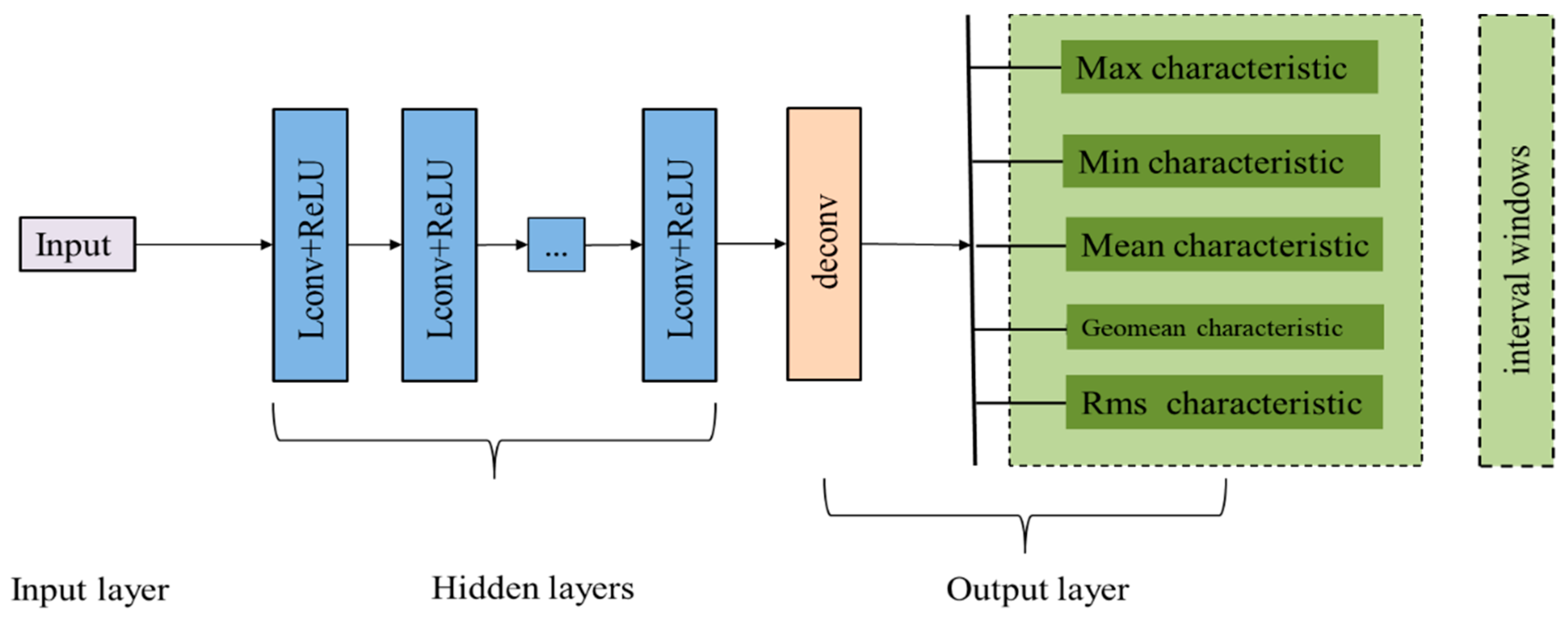
To analyze the characteristics from one–dimensional current data of appliances, CNN and LPBoost are combined to extract features in this subsection. We propose a 1D convolutional neural network (1D–CNN) for load monitoring and decomposition. One can see the structure of 1D–CNN from the following Figure 2.

• For the input, input data are the original current of the appliance measured by a meter over a period of time, containing single–appliance and multiple–appliance. Meanwhile, the current data must be obtained during the use of electrical appliances;
• For each hidden layer, the 1D convolution values are calculated by the Lconv function and a one–dimensional convolution kernel, and then they will be activated by the function ReLU;
• For the output layer, the interval windows are applied to extract characteristics from the result of hidden layers, which are transient characteristics. Here the optimal window width is obtained by the smoothing technique in [45]. In the hidden layers, we have the 1D convolution function Lconv;

  $$\widehat{w}=conv\left(u,v\right)$$

  (1)

  where $\widehat{w}$ represents the convolution value, and conv(.) denotes the convolution operator and the vectors, u and v, respectively, denote the convolution kernel and the current of appliances. We take the stride as 1, which means the step size of the convolution calculation.

In the output layers, we have the 1D convolution function Lconv,

$$w=deconv\left(\widehat{w},v\right)$$

(2)

where w represents the deconvolution value, which means the output value filtrated by the convolution operator, and deconv(.) denotes the deconvolution operator.

According to the GoogLeNet [27], for each hidden layer, we have constructed the initial 1D convolution kernel:

• For the input, the kernel is

  $$u_1^i=A_{1\times 3}^i,i=1,2,3$$
• For the second hidden layer, the kernel is

  $$u_2^i=A_{{}_{1\times 5}}^i,i=1,2,\dots ,5$$
• For the Dth hidden layer, the kernel is

  $$u_D^i=A_{1\times D}^i,i=1,2,\dots ,2\mathrm{D}+1$$

  where $A_{1\times j}^i$ denotes the size of the kernel vector is 1 row j column.

In each layer, of the 1D–CNN, we apply the activation function ReLU [42] to obtain the value for the next layer,

$$\mathrm{ReLU}\left(\widehat{w}\right)=max(0,\widehat{w})$$

(3)

To avoid the influence of the negative current characteristics caused by the convolution operation on the identification of the appliance, we used the ReLU activation function to adjust the output data.

Then for the input layer, the hidden layers and the output layer, the specific algorithms are as follows

$$f_1(x)=x;$$

$$f_i(x)=\mathrm{ReLU}(B_{i-1}{f}_{i-1}(x)+b_{i-1}),i=2,3,\dots ,D;$$

(4)

$$f_{D+1}(x)=\mathrm{ReLU}(f_D).$$

Here, x is the value of the input vector after convolution option, B_i and b_i are the weights and basis with kernels at Layer i.

Taking some hidden layers as an example, we exhibit the detailed structure of 1D–CNN based on GoogLeNet, which could improve the recognition accuracy of the load monitoring and decomposition.

In Figure 3, the Lc_ij denotes the value of the convolution operation for the ith hidden layer and j order convolution kernel.

When the power system that NILM needs to detect includes multiple unknown appliances, because of the mutual interference between different appliance current data, it is difficult to identify the corresponding appliance by the characteristics of the appliance current. Then, some techniques are needed in NILM to amplify the difference in current data characteristics of different appliances. In this paper, 1D–CNN is constructed to narrow this difference, taking Figure 4 as an example.

As shown, the subfigure (a) represents the original current data, and the subfigure (b) represents data processed by 1D–CNN. As can be seen by the blue and black rectangles in Figure 4a, the current data in the blue rectangle has some interference with the current data in the black rectangle, which means that there is a coincident portion between them. On the contrary, the degree of difference between the processed current data is more obvious in Figure 4b, which is mainly manifested in the fact that the current data of different color rectangles hardly have an influence of increasing or decreasing each other. Meanwhile, the current data exhibits a regular change. In order to extract the specific characteristics of the processed appliances at different times, this paper mainly uses the interval window mode to analyze the current characteristics of the electrical appliances in a continuous–time. This step mainly consists of two parts, one is the specific mode of the interval window, and the other is the model for extracting the current characteristics in the interval window.

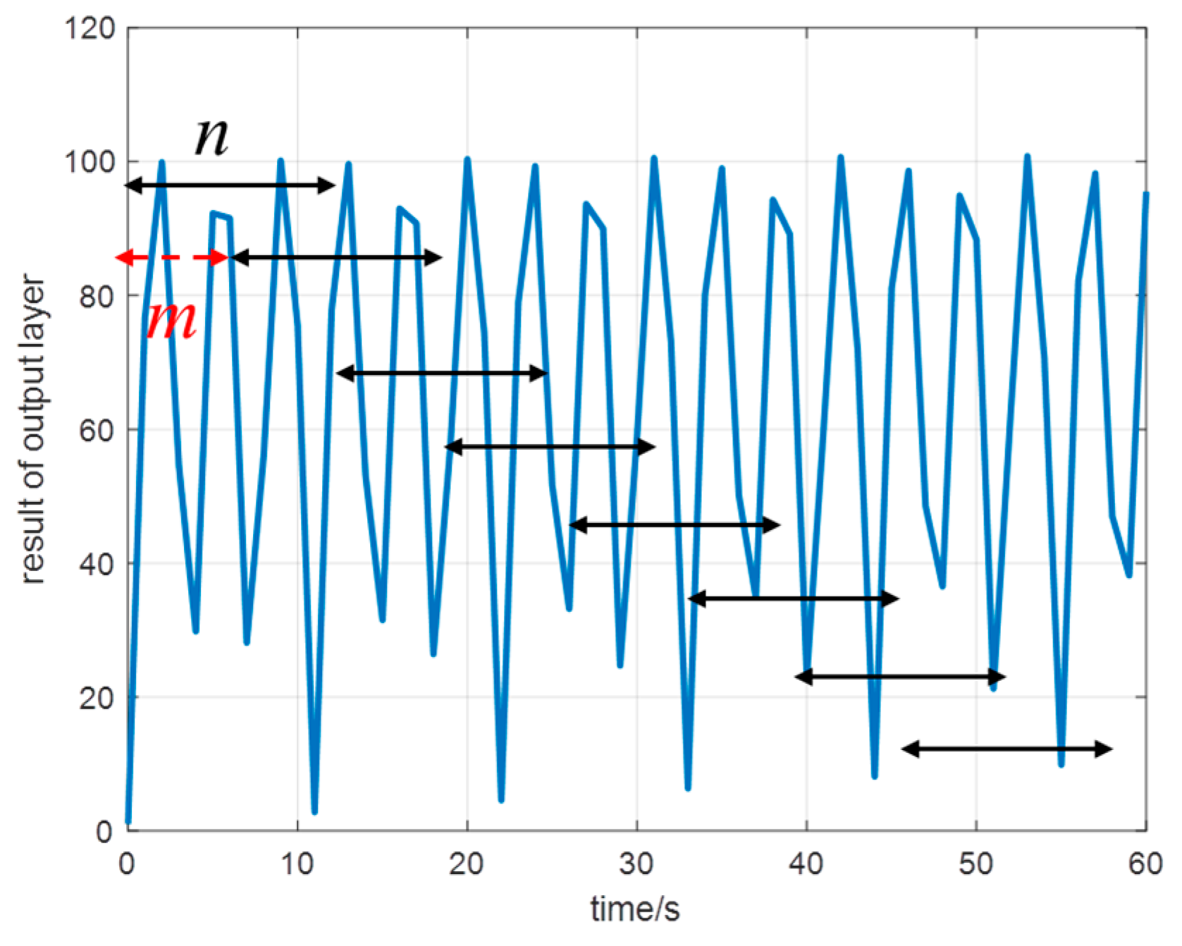
For the interval window, when the current characteristic is analyzed by the interval window, the specific function is to divide the processed complete current data segment into a plurality of independent data segments according to the setting step size. Then it can extract and analyze the current characteristics separately in the independent segments. The specific form of the interval window is as follows:

First, each of the two–way arrows in Figure 5 represents a spacing window, and the length of the spacing window is fixed as n. At the same time, the moving distance, which is step size, between all the adjacent two spaced windows is a fixed value as m. Here, the optimal window width is obtained by the smoothing technique in [45]. The interval windows’ detail is shown in Figure 5.

After the processed current exhibits some regular changes, in order to perform electrical identification, it is necessary to analyze the statistical characteristics of these changes in the internal window. This approach not only reduces the amount of data but also extracts features that have a more positive impact on NILM, as reflected in the accuracy of appliance identification, which is reflected in the experimental section. Based on the above, the 1D–CNN in the TNILM system uses statistical features such as max, min, avg, rms, and geomean to summarize the current characteristics for load monitoring and decomposition, which are obtained from the results of the hidden layer. The function is as follows,

$$V_{\max }^i=\max (w_i)$$

$$V_{\min }^i=\min (w_i)$$

$$V_{avg}^i=\frac{1}{N}{\displaystyle \sum _{i=1}^N{w}_i}$$

(5)

$$V_{rms}^i=\sqrt{\frac{1}{N}{\displaystyle \sum _{i=1}^N{w}_i^2}}$$

$$V_{geomean}^i=\sqrt[N]{{\displaystyle \sum _{i=1}^N{w}_i^2}}$$

where w_i is the value of the output of the hidden layers with the interval window of i length, i denotes the specific sequence in the vector extracted by 1D–CNN. The running mark of each appliance is a series of data, but its characteristics are mainly reflected at certain time points. So in order to identify the appliance more reasonably and effectively, we adopt the mode of the interval window. And the characteristics with the subscripts max, min, avg, rms, geomean, denote the maximum, minimum, average, root mean square, the geometric mean value in an interval window for current data, respectively.

The result of the 1D–CNN is shown in the following Figure 6.

3.2. Adaptive Linear Programming Boosting

Given the transient characteristics calculated by 1D–CNN, the original current has been transformed into a matrix with five rows and multiple columns after being processed by an internal window, which is presented as follows.

$$X_{1\times n}\to X_{5\times m}$$

where n > m, $X_{1\times m},X_{2\times m},X_{3\times m},X_{4\times m}$ and $X_{5\times m}$ respectively denote the max, min, avg, rms, and geomean transient characteristics.

Then the input and output data of the second step can be denoted as follows.

$$(X_{1,i},X_{2,i},X_{3,i},X_{4,i},X_{5,i})\to y_i$$

where y_i denote the appliance estimated by the second step.

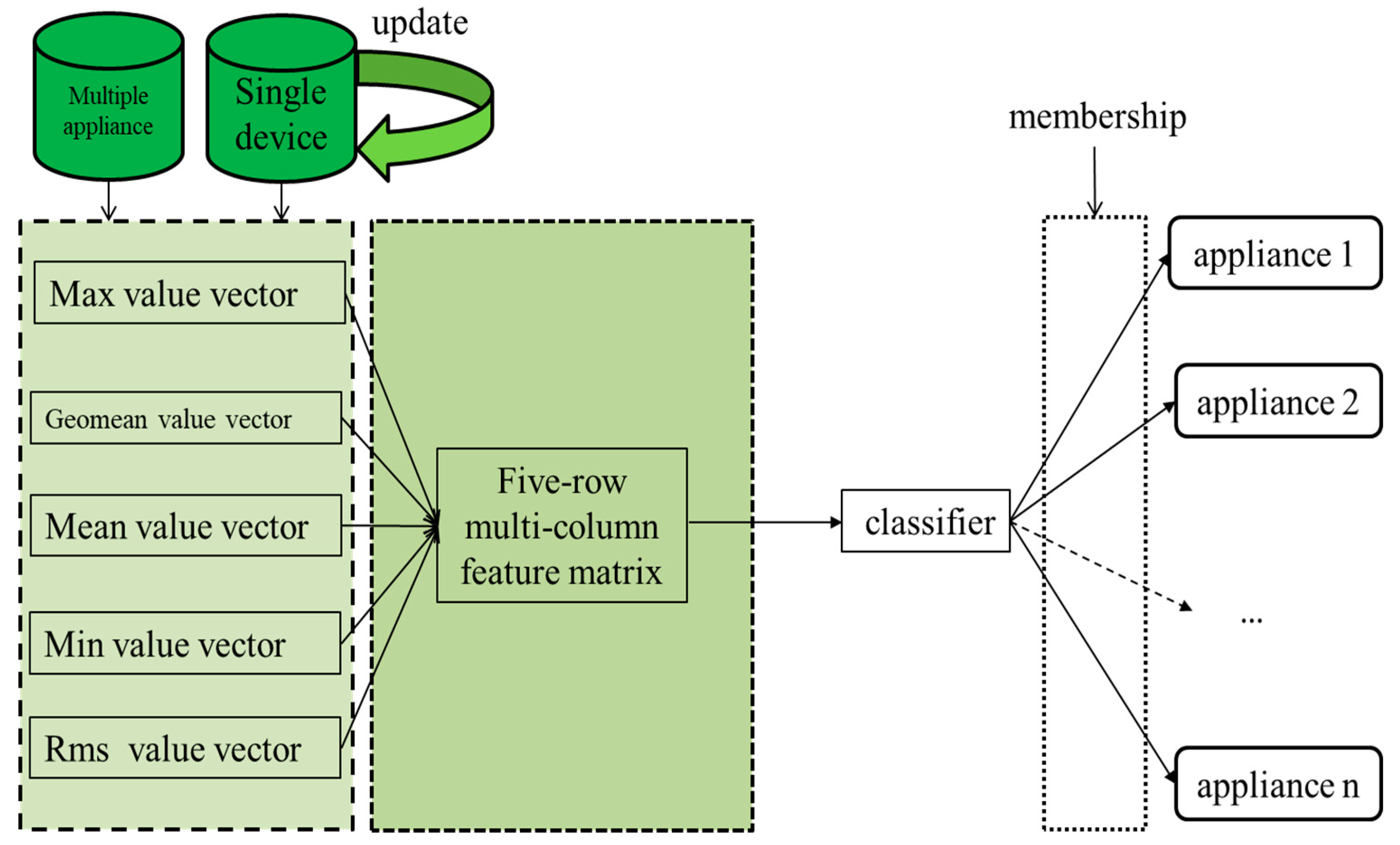
For load monitoring, a novel multi–label classifier (recognizer) has been constructed, which is applied as the second step of the system, which the process is roughly shown in Figure 7.

Most traditional classification methods just apply non–integrated classifier in nonintrusive load monitoring system, such as KNN, BP ([14,15,30], etc.), bagging, and boosting [46] etc. In order to improve the classification accuracy, ensemble learning is applied in this paper for the second step of TNILMD. The experimental results of the comparison presented in Section 4 show that ensemble learning can effectively improve the accuracy in the processing of load monitoring compared to a single classifier. We adopt the improved Adaptive Linear Programming Boosting (ALPBoost) based on Linear Programming Boosting (LPBoost), see Algorithm 2. Compared with LPBoost, the ALPBoost has the following improvements:

• Changing fixed weights into adaptive weights in I: Initiation of Algorithm 2;
• Changing fixed thresholds into adaptive thresholds for single–appliance and multiple–appliance identification in II: Iterate of Algorithm 2;
• Adding two steps to determine the type of appliance with the III: Identification in Algorithm 2, given the value ${\rho }_n$, the detail will be presented in Algorithm 2.

Algorithm 2: ALPBoost

Input:     Training set X = {x1, x2,…,xl}, xi∈X     Training labels Y = {y1, y2,…,yl }, yi∈{−1,0,1} Output:     Classification function f: X→{−1,0,1} I: Initiation:     1: Construct normalized weights: ${\lambda }_n$←$\frac{n}{{\displaystyle \sum _{n=1}^{l}n}}$, n = 1,2,…,l;     2: Construct the objective function: $\widehat{h}\leftarrow \underset{w\in \mathsf{\Omega }}{\arg \max }{\displaystyle \sum _{n=1}^t{y}_{n}h}$(xn;w)${\lambda }_n$;     3: Initialization the objective function value: $\gamma$←0;     4: Initialization iterations count: J ←1; II. Iteration   Adaptive convergence threshold ${\theta }_j\in \theta$ $(j=1,2,\dots ,N)$, N represent the number of iterations;   if ${\theta }_j{\displaystyle \sum _{n=1}^t{y}_n\widehat{h}}$(xn;w)${\lambda }_n$+${\gamma }_t$≤ θj (j = 1,2,..,N) then break;     1: Update the objective function: hJ ← $\widehat{h}$;     2: Update iterations: J ← J + 1;     3: Update the objective function value: ${\gamma }_t\leftarrow {\gamma }_{t+1}$;     4:$(\lambda ,{\gamma }_t)$ ← solution of ALPBoost dual;     5: α ← Lagrangian multipliers of solution to ALPBoost dual problem; III: Identification     1: Construct classification function: mn ← count(sign(${\displaystyle \sum _{j=1}^J{\alpha }_j{h}_j(x)}$) = 1);     2:${\rho }_n=\frac{m_n}{M_n}$ (if mn ≥ Mn, ${\rho }_n$ = 1) ← the membership of appliance;     3: if ${\rho }_n$∈ (${\rho }_{-}^n,{\rho }_{+}^n$) then x is the appliance j.

Note: if the convergence threshold θ is set to be 0, the obtained solution will be the optimal global solution. In practice, θ is set to a small positive value to obtain a good solution as soon as possible. For part III of Algorithm 2, m_n is the total number of matching point in the region, which means the number of sign(${\displaystyle \sum _{j=1}^J{\alpha }_j{h}_j(x)}$ ) = 1; M_n is the total point of training labels data; ${\rho }_{-}^n,{\rho }_{+}^n$ denote the lower and upper bounds of membership respectively. ${\rho }_n$ is the membership for appliance j. When ${\rho }_n$ meets the requirement that (${\rho }_{-}^n,{\rho }_{+}^n$), it can say that multiple–appliance includes appliance j.

For the input data of Algorithm 1, x_i = {$x_i^1,x_i^2,x_i^3,x_i^4,x_i^5$} denotes the max/min/avg/rms/geomean transient characteristics respectively, as shown in Figure 8. The value of y_i are taken to be {−1, 0, 1}, which denote fault–monitored, unmonitored and properly monitored appliances’ operating point respectively.

3.3. Parameter Update

To improve the accuracy of the model, an update function is constructed, which is mainly utilized to update the parameters of 1D–CNN and ALPBoost. This process needs to create a new loss function, and the goals of the updated processing are mainly aimed at the characteristics and classification accuracy. Then according to the 1D–CNN and ALPBoost, we have the loss function

$$f(c;x,\widehat{x})=\frac{1}{n}{\displaystyle \sum _{i=1}^n{(x_i-{\widehat{x}}_i)}^2}+J(c)$$

(6)

$$J(c)=\frac{\lambda }{2}{\Vert c_1+c_2\Vert }^2$$

(7)

where for the first term of $f(x)$, $\frac{1}{n}{\displaystyle \sum _{i=1}^n{(x_i-{\widehat{x}}_i)}^2}$ is mainly applied to evaluate the classification accuracy of the proposed method and x_i is the actual label of the appliance, ${\widehat{x}}_i$ is the classification output of I given by the TNILM. Here, x_i and ${\widehat{x}}_i$ are both binary variables. For the second term of $f(x)$, $J(w)$ is the L₂ regulation for 1D–CNN and ALPBoost to avoid overfitting in the training process, c₁ and c₂ denote the parameters for 1D–CNN and ALPBoost respectively, and $\lambda$ is the regularization coefficient.

The gradient corresponding to the Equation (6) is

$${\nabla }_w\tilde{f}(c;\mathit{x},\widehat{\mathit{x}})={\nabla }_{c}f(c;x,\widehat{\mathit{x}})+\lambda \Vert c_1+c_2\Vert$$

Then we can use the single–step gradient descent to update weights, that is

$$c\leftarrow c-\mathsf{\Gamma }(\lambda c+{\nabla }_{c}f(c;x,\widehat{x}))$$

where $\mathsf{\Gamma }$(.) denotes the update process for parameters.

In the training process, the characteristics of the corresponding position will change along with the parameters. In order to ensure the stability of the method, an extra item must be added to guarantee that the updated feature value remains within a suitable range.

$$g(X)={\displaystyle \sum _{i=1}^{m-1}\left|X_{i+1}-X_i\right|}$$

(8)

where X_i (X_i = (max_i, min_i, mean_i, rms_i, geomean_i)) denote the vector containing five features, then two thresholds are assured to maintain the stability and accuracy for proposed method.

The pseudo–code of the update process is as shown in Algorithm 3.

Algorithm 3: update process

$\begin{array}{l}if\hspace{0.17em}\hspace{0.17em}(g(X)>\delta \hspace{0.17em}\hspace{0.17em}or\hspace{0.17em}\hspace{0.17em}A<\sigma )\hspace{0.17em}\hspace{0.17em}do\\ \hspace{0.17em}\hspace{0.17em}\hspace{0.17em}\hspace{0.17em}f(c;x,\widehat{\mathit{x}})=\frac{1}{n}{\displaystyle \sum _{i=1}^n{(x_i-{\widehat{x}}_i)}^2}+J(c)\hspace{0.17em}\hspace{0.17em}\\ \hspace{0.17em}\hspace{0.17em}\hspace{0.17em}\hspace{0.17em}c\leftarrow c-\mathsf{\Gamma }(\lambda c+{\nabla }_{c}f(c;x,\widehat{\mathit{x}}))\\ else\hspace{0.17em}\hspace{0.17em}do\\ \hspace{0.17em}\hspace{0.17em}\hspace{0.17em}\hspace{0.17em}c\leftarrow c\\ end\end{array}$

Here $\delta$ is the threshold to maintain the stability of method, and $\sigma$ is the threshold to maintain the accuracy of method.

4. Experiment Results

The waveform of the real industrial current data is different from the laboratory data because of the influence of measuring the time interval. Many existing methods will handle the current signals through filtering operations, but it is not suitable as an operating link in smart grid technology. For the rigor of the results, we denoise the data by the proposed method [47]. In this paper, we adopt the current data of AC power to verify the effectiveness of the proposed method, which comprises single–appliance and multiple–appliance, including two, three and five different appliances. The standard frequency of the Alternating Current (AC) power supply is 50 Hz and the rated voltage is 220 V. And the current sampling interval is one second. Taking a real current of decomposition as an example, its waveform is shown in Figure 9. The data in this article were obtained in a high–level graduate data mining competition, which is open access.

Figure 9a presents the current waveform of multiple–appliance, including the appliances: fan, microwave oven, and laptop. The current waveforms are presented in Figure 9b–d.

The recognition of a single appliance is exceptionally simple, and load monitoring can be performed directly by extracting a cycle of features. However, it can be seen from Figure 9 that for hybrid appliances, the load monitoring is more difficult. Therefore, we apply our method proposed in Section 3 to make the load monitoring.

To normalize current data before starting training and testing with the system, we have the function.

$$x=2*\frac{x-x_{max}}{x_{max}-x_{min}}-1$$

(9)

where x_max, x_min present the maximum and minimum value of current x, respectively.

As shown in Figure 10, the multiple–appliance includes the fan, microwave, and laptop. From the waveform of change in the amount of current, it is difficult to distinguish which appliances are present in the hybrid device. In this paper, 1D–CNN is used to extract the characteristics of current changes. Among them, subfigure (a) denotes the original waveform changes; subfigure (b) denotes the five characteristics for current data, subfigure (c) shows the maximum characteristics of current for a cycle of interval window; subfigure (d) shows the minimum characteristics of current for a cycle of interval window; subfigure (e) shows the average characteristics of current for a cycle of interval window; subfigure (f) shows the square root of geometry characteristics of current for a cycle of interval window; and subfigure (g) shows the geometric average characteristics of current for a cycle of interval window. These characteristics can all be attributed to the transient characteristics of the current [2,47].

However, it is awkward and difficult to discriminate only through the five typical characteristics extracted by 1D–CNN. Therefore, this paper uses this improved adaptive LPBoost (ALPBoost) to discriminate which appliance, which is an ensemble learning method and has been described in Section 3.2.

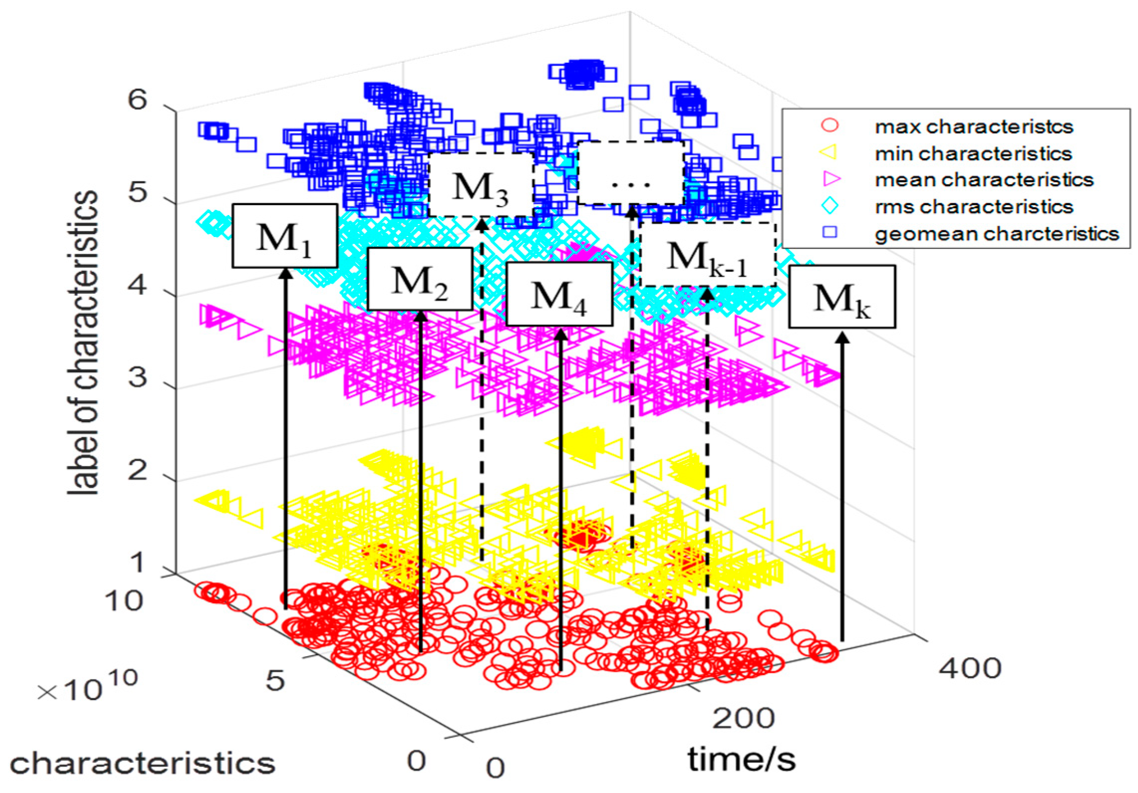
As shown in Figure 11, the direction of the black arrow is perpendicular to the xoy plane. The corresponding feature of the label in the direction of each black arrow is the training data of ALPBoost. The output value M_i of the corresponding arrow is the degree of membership for appliance of the feature vector.

4.1. Single–Appliance Identification of TNILM

For the single appliance identification, the TNILM system utilizes the five characteristics extracted by 1D–CNN to judge the type of single appliance by ALPBoost. Meanwhile, to update the parameters of 1D–CNN and ALPBoost, the parameter update process is applied. In this case study 1, 11 kinds of single appliances are used to verify the feasibility of the system, which including Fan, Microwave, Kettle, Laptop, Incandescent, Energy Saving Lamp, Printer, Water Dispenser, Air Conditioner, Hair Dryer and TV. Appliances can be divided into the following three types depending on the working status of the appliances: (1) ON/OFF two–state appliance; (2) Limited multi–state appliance. This kind of appliance usually has a limited number of discrete operating states; (3) Continuous variable state appliances. The steady–state section power of this type of appliance has no constant mean value, but a continuous change in the range. In this experiment, current data samples from 300 single appliances were used to train, which includes 11 appliance types, as shown in column 1 of

Table 2. The single–appliance recognition rate of TNILM.

No	Appliance	Training Accuracy (%)	Testing Accuracy (%)
1	Fan	97.1	95.8
2	Microwave	97.3	93.6
3	Kettle	100	100
4	Laptop	95.5	93.3
5	Incandescent	96.3	94.0
6	Energy saving lamp	96.4	93.2
7	Printer	98.0	95.5
8	Water dispenser	100	98.8
9	Air conditioner	98.5	95.1
10	Hair dryer	100	100
11	TV	97.5	94.2

Note: for the training accuracy and test accuracy, the paper evaluates the performance of the algorithm according to the F1–score of methods.

. Meanwhile, 60 data samples of single–appliance are used to test. The recognition accuracy for single–appliance of our system has been denoted in Table 2.

As shown in Table 2, when we apply the TNILM system to recognize appliances, the training accuracy of 11 kinds of single appliances can reach about 95–100% and the testing accuracy of single–appliances can even reach 90%. For appliances with only OFF/ON two statuses (e.g., Kettle and Water dispenser), the recognition accuracy is relatively high, and for the others taking few statues (e.g., Microwave and Laptop), the recognition accuracy is relatively low. In addition, when the operating characteristics of some appliances are similar (e.g., Incandescent and Energy–saving lamp), their identification accuracy will be relatively low due to mutual interference. In general, the accuracy is acceptable. Therefore, the TNILM is effective and reasonable for single–appliance identification.

In order to further verify the effectiveness of the characteristics extracted by the 1D–CNN and the advanced nature of the ALPBoost in load monitoring, we have combined the characteristics extracted by the 1D–CNN with a variety of classifiers to replace ALPBoost to perform recognition accuracy analysis. The specific results are shown in

Table 3. Comparison of different classifiers for single–appliance recognition rates.

No	Classifier	Training Accuracy (%)	Testing Accuracy (%)
1	SVM	90.2	87.3
2	KNN	92.5	90.6
3	Random Forest	93.4	91.6
4	AdaBoostM2(tree) [48]	95.5	92.8
5	LPBoost(tree)	96.1	93.7
6	ALPBoost	97.7	95.4

Note: for the training accuracy and test accuracy, the paper evaluates the performance of the algorithm according to the F1–score of methods.

.

For single–appliance identification, comparing our classifier with other classifiers, e.g., SVM, KNN, Random Forest [49], AdaBoostM2 (tree) [50], and LPBoost (tree), the compared results of the average identification accuracy are denoted in Table 2. It turns out that the effect of our classifier ALPBoost is higher. In addition, the results demonstrate that all classifiers obtain a good classification result, respectively. The identification effects of ensemble classifiers containing Random Forest, AdaBoostM2 (tree), and LPBoost (tree) is better than traditional classifiers containing SVM and KNN. On the other hand, the classification effect of all classifiers can reach 90%, which proves the effectiveness of 1D–CNN and Parameters update processing in extracting features.

4.2. Multiple–Appliance Identification of TNILM

In real world, whatever commercial activity or residential activity, there are relatively many cases where multiple appliances work together account at a certain time, so the amount of data in this area is large. For the smart grid, the problem that the non–intrusive load monitoring system has to meet is also this situation.

In this case study, for the load monitoring of multiple–appliance identification, assuming that multiple–appliances contain 11 types of single appliances, the detail has been described in Section 4.2. Meanwhile, we have considered other appliances, that is, unmentioned appliances in Section 4.2, which are labeled as No0. For the further study of appliances, which have not been mentioned yet, you only need to apply TNILM to uniformly update their characteristics into the database by its current waveform of the appliance. Taking into account the calculation accuracy and computing resources, this experiment employed the current data of 500 multiple–appliances including two, three, and five different appliances in the multiple–appliance of the family for training and the current data of 100 multiple–appliances for testing. Take several typical multiple–appliances as an example, the specific results analysis are shown in

Table 4. Multiple–appliance types.

Type	Real Including Appliances	Predict Including Appliances	Hypothetical Accuracy (%)
1	Kettle, Printer	Kettle, Printer	100
2	Fan, Microwave, Laptop	Fan, Microwave, Laptop	100
3	Energy saving lamp, Water dispenser, Hair dryer	No12, Water dispenser, Hair dryer	66.7
4	Laptop, Incandescent, Water dispenser, Hair dryer, TV	Laptop, No12, Water dispenser, Hair dryer, TV	80.0
5	Kettle, Laptop, Incandescent, Printer, Air conditioner	Kettle, Laptop, Incandescent, Printer, Air conditioner	100
6	No0, Microwave, Hair dryer	No12, Microwave, Hair dryer	80
7	No0, Laptop, Incandescent, Water dispenser, Air conditioner	No0, Laptop, No12, Water dispenser, Air conditioner	80

Note: for the hypothetical accuracy, the paper evaluates the performance of the algorithm according to the F1–score of methods.

. We labeled the misidentified appliances as No12.

As shown in Table 4, the recognition rate of multiple–appliance of Type1, Type2, and Type5 is 100%, which can be classified into one type. The recognition rate of multiple–appliance of Type3 and Type4 is 66.7% and 80%. They all identify mentioned appliances as other mentioned appliances, which can be classified into another type. And the non–identified appliances are included in 11 kinds of appliances in above. A multiple–appliance with a No6 recognizes the appliance is labeled No0 as one of the 11 appliances in above, which the accuracy is 80%. A multiple–appliance of Type7 can effectively recognize the device No0 that has not been mentioned. However, it recognizes a mentioned appliance as being erroneous, which is denoted as No12.

The results of the recognition rate of the system proposed in this paper on multiple–appliance are shown in

Table 5. The multiple–appliance recognition rate of TNILM.

Type	N	Training Accuracy (%)	Testing Accuracy (%)
1	2	95.6	92.9
2	3	94.2	91.7
3	5	92.4	90.8
4	total	94.1	91.8

Note: N denotes the number of appliances included in the multiple–appliance.

.

As can be seen from Table 5, the TNILM system has a very good recognition rate when performing load monitoring for multiple–appliance with two, three and five different appliances and its identification accuracy can reach over 90%. Of course, when the number of appliances included in the multiple–appliance increases, the recognition accuracy will be relatively low, and it is the actual situation of industrial data.

Similarly, in order to prove the effectiveness of the proposed system in dealing with non–intrusive problems, we compared the classification effects of various classifiers. The detail is denoted in

Table 6. Comparison of different classifiers for multiple–appliance recognition rate.

No	Classifier	Training Average Accuracy (%)	Testing Average Accuracy (%)
1	SVM	85.6	82.1
2	KNN	82.3	80.5
3	Random Forest	89.6	85.4
4	AdaBoostM2	90.8	88.7
5	LPBoost	92.3	90.5
6	ALPBoost	94.1	91.8

.

For multi–appliance classification, comparing the identification effect of ALPBoost with other classifiers, the results of the average classification accuracy in Table 6 demonstrate that the effect of ALPBoost is higher, and the classification effect of all classifiers can reach 85%. Meanwhile, no matter which kind of classifier the recognition accuracy reaches 80%; this also indirectly proves the validity of the characteristic extracted by 1D–CNN. Comparing Table 2 with Table 5, the results show that when the identification type transitions from single–appliance identification to multiple–appliance identification, the accuracy is reduced about 3–5%, which is acceptable and demonstrates the effectiveness of the TNILM.

As shown in Figure 12, the accuracy of the system gradually increases as the number of updates increases. For single–appliance identification, the number of update times that satisfy the threshold of accuracy (92%) is 7, and for the multiple appliance identification, the number of update times that satisfy the threshold of accuracy (90%) is 15. In order to obtain a better recognition effect, after the threshold condition is met, the system can be updated again.

5. Conclusions

A novel three–step NILM system is presented in this paper to improve the recognition accuracy. The proposed TNILM applies a 1D convolution neural network to detect the characteristics of the appliance and improve the ALPBoost to identify the appliance. The advantage of TNILM is that it not only captures the main features of the transient signals of current but also updates the system in real–time to increase recognition accuracy. Several TNILM were developed and tested for signature identification of appliances based on the current, under industrial data. This is drastically different from other studies. To verify the validity of the proposed nonintrusive system, two different experimental case studies are investigated in this paper. The cases include some of the most challenging scenarios for a NILM system to identify, such as different loads with three different appliance operating states. The results indicate that all methods obtained high classification performance and correctly identified the appliances, establishing the applicability of the proposed approach. Future research will include extending the scope of multiple–appliance and determining the operating status of the appliances at different times, which is a step that must be taken in order to predict the future electricity consumption of users. At the same time, the system proposed in this paper is based on semi–supervised learning. In the future smart grid technology, unsupervised learning is the direction of expansion. We will extend the semi–supervised system to non–supervised systems in the following research.

References

1. Pérez–Lombard, L.; Ortiz, J.; Pout, C. A review on buildings energy consumption information. Energy Build. 2008, 40, 394–398. [Google Scholar] [CrossRef]
2. Bamberger, Y.; Baptista, J.; Belmans, R.; Buchholz, B.M.S.; Chebbo, M.; Doblado, M.; Efthymiou, V.; Gallo, L.; Handschin, E.; Hatziargyriou, N.; et al. Vision and Strategy for Europe’s Electricity Networks of the Future; Office for Official Publications of the European Communities: Luxemburg, 2006. [Google Scholar]
3. Chui, K.T.; Lytras, M.D.; Visvizi, A. Energy sustainability in smart cities: Artificial intelligence, smart monitoring, and optimization of energy consumption. Energies 2018, 11, 2869. [Google Scholar] [CrossRef]
4. Zeifman, M.; Roth, K. Nonintrusive appliance load monitoring: Review and outlook. IEEE Trans. Consum. Electron. 2011, 57, 76–84. [Google Scholar] [CrossRef]
5. Du, S.; Li, M.; Han, S.; Jonathan, S.; Lim, H. Multi–pattern data mining and recognition of primary electric appliances from single non–intrusive load monitoring data. Energies 2019, 12, 992. [Google Scholar] [CrossRef]
6. Hsueh–Hsien, C. Non–Intrusive demand monitoring and load identification for energy management systems based on transient feature analyses. Energies 2012, 5, 4569–4589. [Google Scholar]
7. Froehlic, H.J.; Larson, E.; Gupta, S.; Cohn, G.; Reynolds, M.; Patel, S. Disaggregated end–use energy sensing for the smart grid. IEEE Pervasive Comput. 2010, 10, 28–39. [Google Scholar] [CrossRef]
8. Bergman, D.C.; Jin, D.; Juen, J.P.; Tanaka, N.; Gunter, C.A. Distributed Non–Intrusive Load Monitoring, Innovative Smart Grid Technologies; University of Illinois at Urbana Champaign: Champaign, IL, USA, 2011; pp. 1–8. [Google Scholar]
9. Chang, H.H.; Lian, K.L.; Su, Y.C.; Lee, W.J. Power–spectrum–based wavelet transform for nonintrusive demand monitoring and load identification. IEEE Trans. Ind. Appl. 2014, 50, 2081–2089. [Google Scholar] [CrossRef]
10. Cominola, A.; Giuliani, M.; Piga, D.; Castelletti, A.; Rizzoli, A.E. A hybrid signature–based iterative disaggregation algorithm for non–intrusive load monitoring. Appl. Energy 2017, 185, 331–344. [Google Scholar] [CrossRef]
11. Patel, S.N.; Robertson, T.; Kientz, J.A.; Reynolds, M.S.; Abowd, G.D. At the Flick of a Switch: Detecting and Classifying Unique Electrical Events on the Residential Power Line; Ubicomp: Copenhagen, Denmark, 2007; Volume 4717, pp. 271–288. [Google Scholar]
12. Gillis, J.M.; Alshareef, S.M.; Morsi, W.G. Nonintrusive load monitoring using wavelet design and machine learning. IEEE Trans. Smart Grid 2017, 7, 320–328. [Google Scholar] [CrossRef]
13. Lin, Y.H.; Tsai, M.S. Development of an improved time–frequency analysis–based nonintrusive load monitor for load demand identification. IEEE Trans. Instrum. Meas. 2014, 63, 1470–1483. [Google Scholar] [CrossRef]
14. Chen, F.; Dai, J.; Wang, B.; Sahu, S.; Naphade, M.; Lu, C.T. Activity analysis based on low sample rate smart meters. In Proceedings of the 17th ACM SIGKDD International Conference on Knowledge Discovery and Data Mining, San Diego, CA, USA, 21–24 August 2011; pp. 240–280. [Google Scholar]
15. Rahimi, S.; Chan, A.D.C.; Goubran, R.A. Nonintrusive load monitoring of electrical devices in health smart homes. In Proceedings of the 2012 IEEE International Instrumentation and Measurement Technology Conference, Graz, Austria, 13–16 May 2012; Volume 8443, pp. 2313–2316. [Google Scholar]
16. Srinivasan, D.; Ng, W.S.; Liew, A.C. Neural–network–based signature recognition for harmonic source identification. IEEE Trans. Power Deliv. 2005, 21, 398–405. [Google Scholar] [CrossRef]
17. Chang, H.H.; Chen, K.L.; Tsai, Y.P.; Lee, W.J. A new measurement method for power signatures of nonintrusive demand monitoring and load identification. IEEE Trans. Ind. Appl. 2012, 48, 764–771. [Google Scholar] [CrossRef]
18. Yang, H.T.; Chang, H.H.; Lin, C.L. Design a neural network for features selection in non–intrusive monitoring of industrial electrical loads. IEEE Trans. Syst. Man Cybern. Part A Syst. Hum. 2007, 32, 582–595. [Google Scholar]
19. Hassan, T.; Javed, F.; Arshad, N. An empirical investigation of v–i trajectory based load signatures for non–intrusive load monitoring. IEEE Trans. Smart Grid 2014, 5, 870–878. [Google Scholar] [CrossRef]
20. Gupta, S.; Reynolds, M.S.; Patel, S.N. ElectriSense: Single–point sensing using EMI for electrical event detection and classification in the home. In Proceedings of the ACM International Conference on Ubiquitous Computing, New York, NY, USA, 26–29 September 2010; pp. 139–148. [Google Scholar]
21. Liu, Y.; Chen, M. A review of nonintrusive load monitoring and its application in commercial building IEEE. In Proceedings of the International Conference on Cyber Technology in Automation, Control, and Intelligent Systems, Hong Kong, China, 4–7 June 2014; pp. 623–629. [Google Scholar]
22. Saitoh, T.; Aota, Y.; Osaki, T.; Konishi, R.; Sugahara, K. Current sensor based non–intrusive appliance recognition for intelligent outlet. In Proceedings of the International Technical Conference on Circuits Systems, Computers and Communications (ITC–CSCC 2008), Tottori, Japan, 6–9 July 2008. [Google Scholar]
23. Zoha, A.; Gluhak, A.; Imran, M.A.; Rajasegarar, S. Non–Intrusive load monitoring approaches for disaggregated energy sensing: A survey. Sensors 2012, 12, 16838–16866. [Google Scholar] [CrossRef] [PubMed]
24. Kolter, J.Z.; Batra, S.; Ng, A.Y. Energy disaggregation via discriminative sparse coding. In Proceedings of the International Conference on Neural Information Processing Systems. Curran Associates, Copenhagen, Denmark, 26–29 September 2010; pp. 1153–1161. [Google Scholar]
25. Shao, H.; Marwah, M.; Ramakrishnan, N. A Temporal Motif Mining Approach to Unsupervised Energy Disaggregation: Applications to Residential and Commercial Buildings Twenty–Seventh AAAI Conference on Artificial Intelligence; AAAI Press: Menlo Park, CA, USA, 2013; pp. 1327–1333. [Google Scholar]
26. Kim, H.S. Unsupervised Disaggregation of Low Frequency Power Measurements Eleventh Siam International Conference on Data Mining. In Proceedings of the Eleventh SIAM International Conference on Data Mining, SDM 2011, Mesa, AZ, USA, 28–30 April 2011; pp. 747–758. [Google Scholar]
27. Szegedy, C.; Liu, W.; Jia, Y.; Sermenet, P.; Angulov, D.; Erhan, D.; Vanhockw, V.; Rabinovich, A. Going deeper with convolutions. arXiv 2014, arXiv:1409.4842v1, 1–9. [Google Scholar]
28. Demiriz, A.; Bennett, K.P.; Shawe–Taylor, J. Linear Programming Boosting via Column Generation. Mach. Learn. 2002, 46, 225–254. [Google Scholar] [CrossRef] [Green Version]
29. Ahmadi, H.; Martí, J.R. Load decomposition at smart meters level using eigenloads approach. IEEE Trans. Power Syst. 2015, 30, 3425–3436. [Google Scholar] [CrossRef]
30. Watkins, A.; Timmis, J.; Boggess, L. Artificial immune recognition system (airs): An immune–inspired supervised learning algorithm. Genet. Program. Evolvable Mach. 2004, 5, 291–317. [Google Scholar] [CrossRef]
31. Parson, O.; Ghosh, S.; Weal, M.; Roger, A. Non–Intrusive Load Monitoring Using Prior Models of General Appliance Types. In Proceedings of the Twenty–Sixth AAAI Conference on Artificial Intelligence, Toronto, ON, Canada, 22–26 July 2012; pp. 356–362. [Google Scholar]
32. Saitoh, T.; Osaki, T.; Konishi, R.; Sugahara, K. Current sensor based home appliance and state of appliance recognition. SICE J. Control Meas. Syst. Integr. 2010, 3, 86–93. [Google Scholar] [CrossRef]
33. Yang, G.; Huang, T.S. Human Face Detection in Complex Background. Pattern Recognition. 1994, 27, 53–63. [Google Scholar] [CrossRef]
34. Tsai, M.S.; Lin, Y.H. Modern development of an adaptive non–intrusive appliance load monitoring system in electricity energy conservation. Appl. Energy 2012, 96, 55–73. [Google Scholar] [CrossRef]
35. Johnson, M.J.; Willsky, A.S. Bayesian nonparametric hidden semi–Markov models. J. Mach. Learn. Res. 2012, 14, 673–701. [Google Scholar]
36. Parson, O.; Ghosh, S.; Weal, M.; Rogers, A. An unsupervised training method for non–intrusive appliance load monitoring. Artif. Intell. 2014, 217, 1–19. [Google Scholar] [CrossRef]
37. Lin, Y.H.; Tsai, M.S. Non–Intrusive load monitoring by novel neuro–fuzzy classification considering uncertainties. IEEE Trans. Smart Grid 2014, 5, 2376–2384. [Google Scholar] [CrossRef]
38. Du, L.; Restrepo, J.A.; Yang, Y.; Harley, R.G.; Habetler, T.G. Nonintrusive, Self–organizing, and probabilistic classification and identification of plugged–in electric loads. IEEE Trans. Smart Grid 2013, 4, 1371–1380. [Google Scholar] [CrossRef]
39. Kolter, J.Z.; Johnson, M.J. REDD: A public data set for energy disaggregation research. SustKDD 2011, 9. [Google Scholar]
40. Guo, Z.; Wang, Z.J.; Kashani, A. Home appliance load modeling from aggregated smart meter data. IEEE Trans. Power Syst. 2014, 30, 254–262. [Google Scholar] [CrossRef]
41. Wang, Z.; Zheng, G. Residential appliances identification and monitoring by a nonintrusive method. IEEE Trans. Smart Grid 2012, 3, 80–92. [Google Scholar] [CrossRef]
42. Zeile, M.D.; Fergus, R. Visualizing and Understanding Convolutional Networks European Conference on Computer Vision; Springer: Cham, Switzerland, 2014; pp. 818–833. [Google Scholar]
43. Krizhevsky, A.; Sutskever, I.; Hinton, G.E. ImageNet classification with deep convolutional neural networks. In Proceedings of the International Conference on Neural Information Processing Systems. Curran Associates, Lake Tahoe, Nevada, 3–6 December 2012; pp. 1097–1105. [Google Scholar]
44. Haykin, S.; Kosko, B. Gradient Based Learning Applied to Document Recognition IEEE; Wiley–IEEE Press: Hoboken, NJ, USA, 2009; pp. 306–351. [Google Scholar]
45. Härdle, W.; Müller, M.; Sperlich, S.; Werwatz, A. Nonparametric and Semiparametric Models; Springer–Verlag: Berlin/Heidelberg, Germany, 2004. [Google Scholar]
46. Quinlan, J.R. Bagging, boosting. In Proceedings of the Thirteenth National Conference on Artificial Intelligence, Oregon, Portland, 4–8 August 1996; pp. 725–730. [Google Scholar]
47. Ridi, A.; Gisler, C.; Hennebert, J. A Survey on Intrusive Load Monitoring for Appliance Recognition[C]// 2014 22nd International Conference on Pattern Recognition (ICPR). IEEE Comput. Soc. 2014, 94, 3702–3707. [Google Scholar]
48. Rätsch, G.; Onoda, T.; Müller, K.R. Soft margins for AdaBoost. Mach. Learn. 2001, 42, 287–320. [Google Scholar] [CrossRef]
49. Liaw, A.; Wiener, M. Classification and regression by random forest. R News 2002, 23, 18–22. [Google Scholar]
50. Schapire, R.E. Improved boosting algorithms using confidence–rated predictions. Mach. Learn. 1999, 37, 297–336. [Google Scholar] [CrossRef]
Figure 1. The structure of the non–intrusive load monitoring system.
Energies 12 02882 g001
Figure 2. 1D convolution neural network (the Lconv denotes the convolution operation in the convolution layers of 1D–CNN).
Energies 12 02882 g002
Figure 3. The detail of 1D–CNN.
Energies 12 02882 g003
Figure 4. 1D–CNN effect on current data. (a) the original current data; (b) the current data processed by 1D–CNN.
Energies 12 02882 g004
Figure 5. Interval windows (The abscissa indicates the time point of the current, and the ordinate indicates the current characteristic after the process.).
Energies 12 02882 g005
Figure 6. The output of 1D–CNN. (a) the original current of the appliance; (b) the current data processed by 1D–CNN; (c) the current data’s maximum characteristics processed by 1D–CNN.
Energies 12 02882 g006
Figure 7. Multi–label classifier based on Adaptive Linear Programming Boosting.
Energies 12 02882 g007
Figure 8. The characteristics extracted from 1D–CNN (in which the data in the black rectangle indicate an input label data for the classifier).
Energies 12 02882 g008
Figure 9. The current waveform of Multiple–appliance and single–appliance. (a) multiple–appliance; (b) fan; (c) microwave oven; (d) laptop.
Energies 12 02882 g009
Figure 10. The characteristics of current of multiple–appliance. (a) the original current data; (b) the five current characteristics of appliances; (c) the maximum current characteristic of appliance; (d) the minimum current characteristic of appliance; (e) the average current characteristic of appliance; (f) the root mean square current characteristic of appliance; (g) the geometric mean current characteristic of appliance.
Energies 12 02882 g010
Figure 11. The result of ALPBoost.
Energies 12 02882 g011
Figure 12. The accuracy of changing of the updating times of TNILM (the accuracy denotes the F1–score).
Energies 12 02882 g012