1. Introduction
Climate change mitigation and adaptation require a profound transformation of the socioeconomic system. This transformation requires actions affecting many different sectors (energy, transportation, agriculture, consumption, production, households, etc.) and scales (from individual-household level to city, province, country, regional, and global levels), and depend on the cultural, historical, political, institutional and governance settings in each particular location. There may be a number of alternatives, each coming with their possible implications. Choosing the best ones is always difficult, and making optimal and robust judgements is challenging since it requires a good understanding of the functioning of complex coupled human and natural systems in a context of high uncertainty [
1,
2]. In many cases we need to carefully assess a variety of different hypothetical combinations of parameters and functions, representing various climatic trends and mitigation or adaptation opportunities and analyze these scenarios at different spatial and temporal scales, often with a diverse set of outputs that are important for stakeholders at relevant levels (local, national, global).
Models are commonly used to understand and analyze a system and its possible future states [
3]. In the context of climate change and, in particular, in the area of low-carbon transitions, there are already many computer models based on various paradigms and approaches. There are hundreds of models that may be relevant for analyzing different dimensions of low carbon transitions. However, it is hardly possible to find a single model that can provide for all alternative climate scenarios at all required levels of complexity.
Global implications of mitigation pathways are extensively explored by Integrated Assessment Models (IAMs) of the climate-economy and energy systems. There is a vast variety of IAMs and many authors have performed comparative reviews of them. For example, a recent review by Nikas et al. [
4] provides comparative information of more than 60 individual IAMs. Connolly et al. [
5] identify 68 (and reviewed 37) models that can be used for integration of renewable energy. Weyant [
6] focuses his review on the analysis of the different uses of IAMs and distinguishes two types of IAMs: detailed process models (used for mitigation analysis, climate impacts analysis, and integrated mitigation and impact analysis), and benefit–cost models (used for computing the optimal trajectory of global greenhouse gas emissions, cost-benefit evaluation of climate policies, and computing the social cost of carbon).
IAMs are very good at tracing feedbacks between global economy as a whole and the climatic system but are heavily criticized for miscalculating the social costs of carbon and omitting cross-sectoral impacts, region-specific characteristics, and endogenous technological change [
7], though progress is being currently made by various research teams to tackle the latter [
8]. Computable General Equilibrium (CGE) models trace cross-sectoral feedbacks of any endogenous or exogenous changes at a country or regional level and their consequences for the economic welfare but are weak in scaling up to global processes. They ignore heterogeneity when using the representative agent paradigm, implying that everyone in a society is the same, makes perfectly informed choices, does not learn and does not change over time. Agent Based Models (ABMs) address these drawbacks and can treat cumulative impacts of behavioral changes and policies for demand side activation. They can model endogenous emergence of technological innovation, but remain confined to local scale because of mounting complexity
While the need for integration is well realized [
9,
10,
11], it is commonly done either through the soft integration of two different models when one alters own parameters based on the scenarios produced by the other [
12] or a re-implementation of functionalities of multiple models within one software package [
13]. Both approaches are a good start. Yet, the vast amount of valuable knowledge that existing simulation models are to offer and the rise of computational methods that make it possible to use them in symbiosis, calls for the development of dynamically-integrated suites of models. The challenge is to link the existing fragmented knowledge and models, capitalizing on the strengths and capabilities of individual components instead of developing new models from scratch each time we are facing another problem. For this we need some methods of integration [
14] that can link the ‘appropriate’ component models into a system-of-systems finding complementarity in these models [
15] and compensating for limitations of one model by what other models may offer [
16]. Such integration bears the promise of better coverage and detail at multiple scales.
Wicke et al. [
17] introduce the concept of “model collaboration” and show how the collaboration between different modeling approaches can provide wider insights into complex research questions involving multiple sectors and disciplines, and different temporal and spatial scales. According to these authors, model collaboration consists of aligning and harmonizing input data and scenarios, model comparison and/or model linkage. The last of these activities is especially challenging, since it requires a relevant effort in terms of integration, harmonization and communication between researches coming from different disciplines, and using a range of modelling approaches.
There are many examples of model linking in the literature, in particular in the field of integrated assessment of climate-energy-economy systems. These studies cover a variety of models (climate models, biophysical models, IAMs, CGE models, partial equilibrium models, etc.) and are applied to many different research topics, the analysis of the physical and economic impacts of climate change combining climate, biophysical and CGE models [
18,
19], the economic analysis of energy transitions linking bottom-up energy models and top-down economic models [
20,
21,
22], linking crop and economic models to analyze climate change impacts [
23], the impacts of sea level rise linking a CGE model and a geographical information system tools [
24], or the health co-benefits of mitigation combining information from IAMs and air quality models [
25,
26,
27]. Finally, apart from the linking exercises, IAMs are in continuous development adopting new features from other models on a regular basis, reducing the needs for modelling linking (e.g., the latest release of the GCAM (v5.1) now includes a water module linked to the agricultural system of the model). Despite of this progress, IAMs are far from being able to individually cover all the dimensions, disciplines, and scales relevant for stakeholders and policy makers.
Model linking is not a simple process and comes with several challenges [
28]. First, we need to identify, access, understand and be able to run individual models to simulate the system we are investigating. This means that we have to translate our research goals into some system modeling exercises and then map this overall modeling effort into a relevant combination of subsystems and submodels that can be useful. In a way, this is like cutting the big picture into a jigsaw puzzle, making some of the pieces similar to what we have in some library or repository. When doing that, we also have to keep in mind that many models are poorly documented [
29], often described only in research papers, which may not present the full capabilities of the models, and may not be sufficient to reproduce the results reported. Commonly we find that much information about a model is stored in modelers’ memories [
30], does not get properly documented, and even when written up tends to assume different terminology, semantics and units, which makes linking of models so time consuming and frustrating. Besides, models may require configuration, parameterization and pre-processing of input data. These stages are very crucial parts of the modeling process but traditionally are most poorly documented. Another challenge of integration is to provide the actual run-time interoperability between independently built models. Synchronization of models depends upon the alignment of time steps and numeric integration methods used in component models, to which results can be quite sensitive [
31]. The optimal settings depend on the specific context of the integration, which can be identified only by running extensive sensitivity analysis for integration schemes as well as for component models.
In addition, one needs to figure out how to validate results and how to present them to the users. Unlike the regular modeling processes, when we have full control over the model and can make modifications if required, in the case of integrated modeling we may be dealing with a semi-closed system, when we may have little or no access to components. An error or an undocumented feature in one of the components can easily propagate through the whole system, generating outputs that will be difficult to interpret and debug. Generic blueprint of interoperability for all kinds of integration is challenging, since research settings are widely diverse among integration projects [
14]. Integration process needs to consider the technical, semantic, and dataset aspects of interoperability.
This paper contributes to the integration modeling efforts by presenting a novel web-platform and illustrating its functionalities by integrating IAM, ABM and CGE energy models. We focus on specific aspects of model integration that pertain to the pre-integration and actual module coupling steps. The specific context of the study comes from linking climate-energy-economy models to investigate different climate change mitigation actions. The model space is taken from the EU FP7 project COMPLEX, which looks at alternative policy options for the transition towards a low carbon society in Europe by 2050 [
32]. The project joined 17 partner institutes and universities across 11 countries in Europe. The COMPLEX suite of models includes a number of models that focus on climate, hydrology, power market simulation, land use, macro-economics, household energy consumption preferences, etc. The spatial coverage of the models ranges from global level to province/household level, with temporal resolutions that go from weeks to decades. One of the objectives of the project was to develop a decision framework—by integrating knowledge and models—that could be used to explore alternative pathways of transition to low carbon economy.
In this paper, we see model integration as an option to explore the complexity of transitions to low-carbon futures and climate change mitigation actions by combining the knowledge represented in several models [
33]. In most cases reported in relevant literature, we find the model integration process to be very case specific, with each model treated individually and linked to specific hand-picked particular models. In our approach, we seek flexibility in the architecture to handle models across scales, - global, regional, and household, - and deal with incomplete, contradictory, and changing requirements and information about the socio-economic system. For this, we strive to simplify and streamline the coupling process allowing models to be swapped if needed. Engaging stakeholders in the process is another essential pre-requisite [
34]. This creates further requirements in terms of model transparency, ease of use and communication of results. One way to remove technical and accessibility constraints and facilitate stakeholder participation is by presenting the models as web applications, making them available through standard web browsers. This led us to using web services to wrap legacy models, converting them into interoperable components. We have also considered component-based, custom-made, and hybrid approaches of model integration [
35]. We preferred the web service-based approach since it allows plug and play type of linking between models regardless of the location and hardware and software platforms of the models. In our framework, the users do not need to install any additional software and can use their web browsers to explore modules as stand-alone components, or build chains of modules by connecting outputs from one module to inputs of other modules. Our goal is to enable non-technical stakeholders to simulate different climate change policy scenarios and improve their understanding of climate-society-environment interactions.
This paper describes the proposed integration process, starting with the pre-integration assessment, then presenting the framework design and, finally, the implementation.
Section 2 discusses how the project members executed the pre-integration assessment process, and how they developed the high-level conceptualization of the integrated system.
Section 3 focuses on the interactions between models.
Section 4 presents how web services provide for interoperability, and it also describes the architecture and implementation of the integration system. We present an example of an integration of an IAM, a CGE and an ABM energy models by means of the online model integration platform developed.
Section 5 discusses the lessons learned from the integration process and how they are relevant for other similar projects.
2. The Pre-Integration Assessment Process: Identifying the Models and Possible Linkages
2.1. What Is Pre-Integration Assessment?
The pre-integration assessment is the first phase of integration in which we identify the participating models and decide whether linking these models can provide scientifically valid output [
35]. Basically, the research objectives define the assessment process. So far, we find it unlikely that the process can be fully automated as it is done for ecosystem services modelling with the ARIES method (ARtificial Intelligence for Ecosystem Services) [
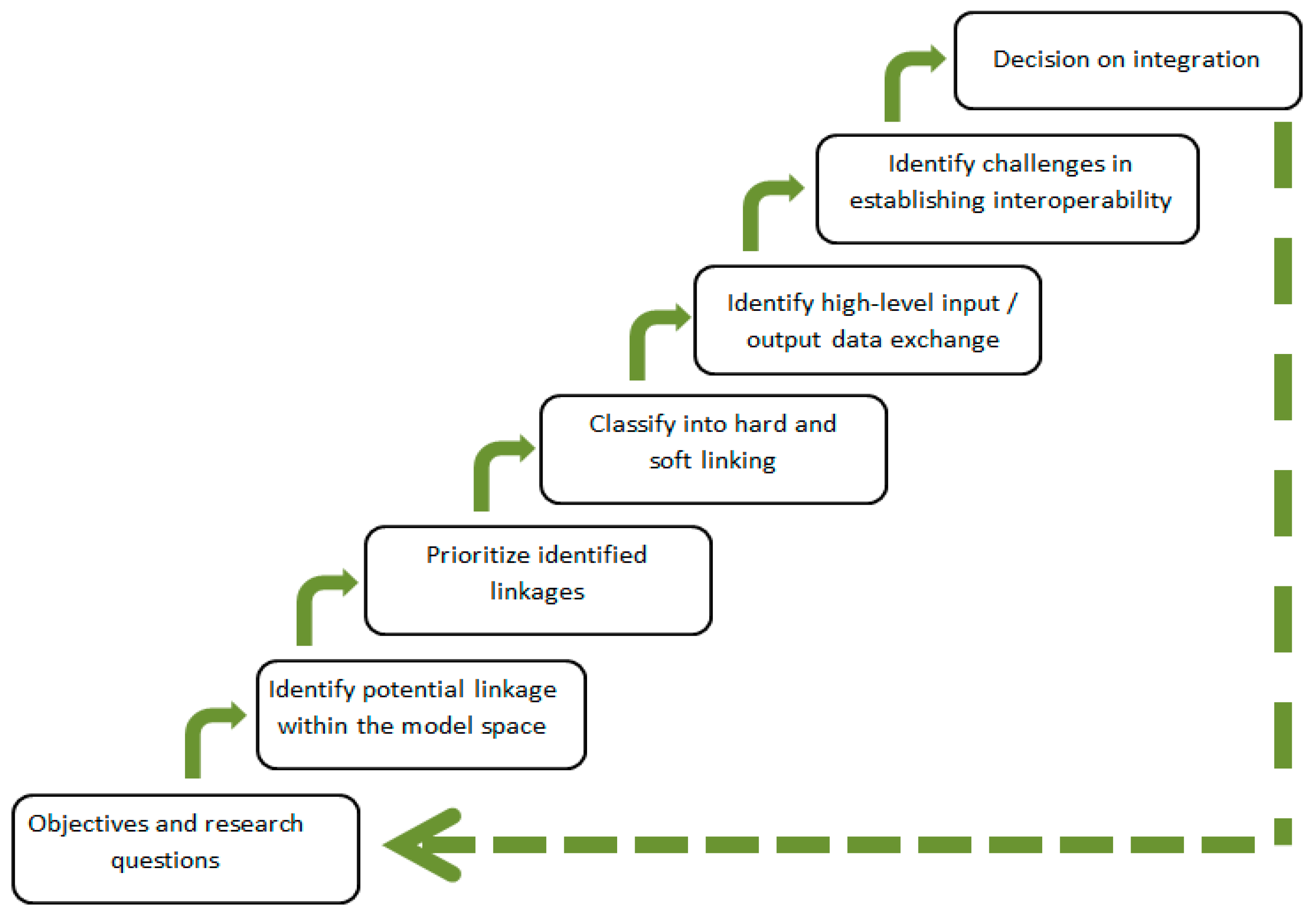
36]: there is still no clear agreement on standards for model documentation, and as a result it is often hard to understand what exactly particular models do and how they are relevant to the project goals. To compensate for lack of standardized documentation we engage in discussions with stakeholders - model owners, developers, and model users who have interest in the integration output. What we can strive for is some sort of computer-aided design, when software tools can assist in informing stakeholders about the candidate models and linkage mechanisms, leaving the final decision to the actual system designers. Generally, the process of pre-integration assessment goes through several steps as indicated in
Figure 1. It is an iterative, highly collaborative process, which requires active participation of all stakeholders.
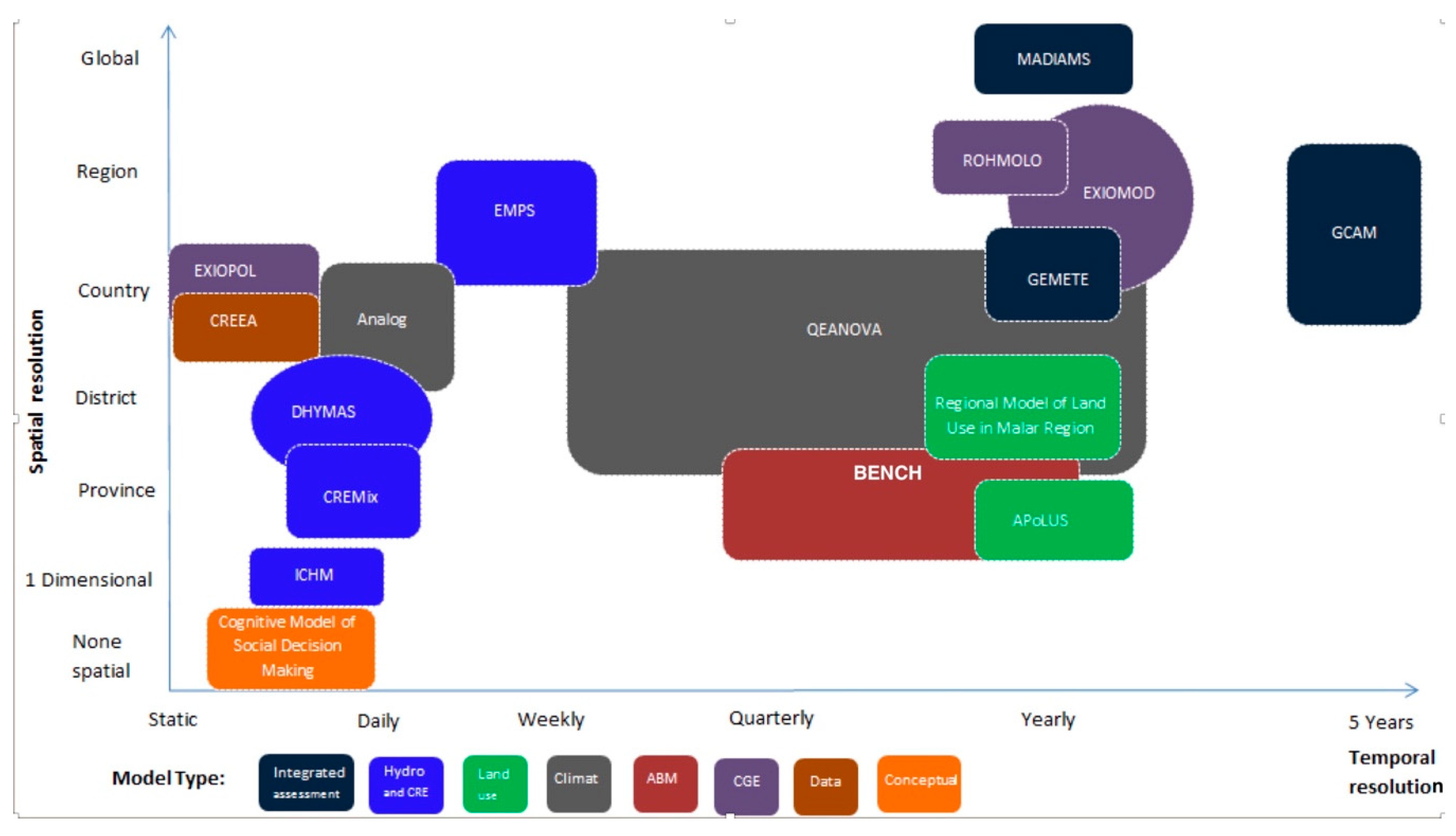
In our case the stakeholders were model developers from the COMPLEX project, all with experience working on applied projects with direct policy relevance. The goal of the pre-integration assessment was to develop a framework that supports climate change mitigation analysis at regional, country, provincial and/or individual levels, if possible, using the models available in the project model space (
Figure 2).
The pre-integration assessment started during a one-day workshop where model owners described what their models do, defined the temporal and spatial scales in which they operate, listed input-output data, described model functionality and assumptions, and the tools used to develop the models. This information was used to explore which output from which models could provide sensible input to other models. The need for ‘better’ input data, which dynamically accounts for feedbacks between modeled systems, is usually the driving factor for linking a model with other models. Ultimately the data exchange between models gives the chance to develop a system-of-systems, which goes beyond the functionality of individual models and rests on previous expertise embedded in other models. By the end of the workshop a number of promising linkages between some models in the COMPLEX repository emerged.
Next, based on our general objective we formulated high-level system requirements that the envisaged integrated system was to address. The goal was ‘To explore the effects of implementing United Nations Framework Convention on Climate Change—UNFCCC -- policy scenarios [
37] in EU27 countries’. According to this convention, emissions of greenhouse gases are to be reduced by 20% by the year 2020; by 40% by 2030; and by 80% by 2050. In the COMPLEX model repository there was a model that could explore how such reductions will affect electricity production. However, changes in electricity production can have significant consequences on other sectors of the economy, and another model from the repository is needed to explore these effects. But it has to be linked to the first model. We need this integrated system to answer such questions as: ‘what will be the effect of a policy in different sectors of the economy?’ or ‘which sectors will be affected most?’ After agreeing on this objective, a number of focused pre-integration assessment meetings were conducted addressing the specific model coupling issues. The information gathered from the meetings was essential to understand how exactly the models had to be linked, prioritize the linkages based on the level of relevance to the project goal, the feasibility, and the resources at hand. Note that the selection of models and the prioritization of linkage points were not at all clear, and required much discussion and some compromise to address all the above-mentioned factors.
Among the available models both GCAM [
39,
40] and EXIOMOD [
41] operate at a global scale and can be used for integrated assessment of energy policies. On the one hand, possible policy scenarios could be fed into GCAM as one of its simulation inputs in order to explore the implications in the energy system (changes in energy consumption/production, energy mix, costs, prices, etc.). On the other hand, EXIOMOD can simulate the macroeconomic and sectoral effects derived from these changes in the energy system. Therefore, by linking GCAM and EXIOMOD we can analyze, in an integrated way, the energy and economic implications of climate policies. In addition, by linking the ABM of the energy market, BENCH [
42], with other macro models it is possible to simulate the cumulative impacts of behavioral changes among households with respect to energy use on the demand side. BENCH complements the two macro models by explicitly modeling micro level dynamics and accounting for behavioral aspects of individual decisions. For example, it can quantify aggregated impacts of behavioral change in the transition to a low carbon economy and track the impacts of information and awareness policies on the residential energy demand, which is commonly difficult to account for a CGE and IAM models [
8]. Besides, since the two macro models operate at country/regional level, linking these models with the household/province level processes represented in BENCH could provide the functionality of analyzing the implications of mitigation policies at different scales. Hence, the three models presented in
Table 1 were selected for the first phase of integration. A detailed description about these models is given in the following sections.
Next, the types of linkages were decided: which models should be hard-linked and where soft-linking is sufficient? In order to differentiate these two concepts, we follow the definitions by Wene [
43]. For this author, soft-linking consists of information transfer controlled by the user and hard-linking involves formal links where information is transferred by computer programs without any user judgment. Accordingly, here, hard linking means creating automated data exchange between models while keeping them separated, and soft-linking means using file-based manual data exchange between models. Further, the hard-link type of integration can be categorized into (1) bi-directional and iterative data exchange between models, which makes intermediate output accessible at the end of each time step; and (2) unidirectional data exchange between models that releases outputs only after the final time step of the model run. Following these discussions, the three models were identified for the hard-linking type of integration, but, due to the differences in the spatial resolution of the models discussed below, EXIOMOD and BENCH were linked bi-directional and GCAM and EXIOMOD uni-directionally. It also became clear that the final decision whether to continue integration or not required more detailed information and further analysis on establishing interoperability between the selected models.
After identifying the participating models, the next step of the pre-integration assessment was the conceptualization of the integrated system and the exploration of the particular input-output data exchange patterns between the models. Spatial and temporal scales of input-output data were also decided. Establishing an automated data exchange between models requires addressing the following challenges:
The mismatch between spatial scales of models. Two models (GCAM and EXIOMOD) operate at the global level but represent the world in a different number of regions/countries. The third model chosen (BENCH) operates in province/household level. The two global models can exchange input-output by aggregating and disaggregating data based on the corresponding spatial scales. To link the provincial level model to EXIOMOD we downscaled the global level output to produce provincial level data for the two selected case study areas.
The need for temporal synchronization of the models. GCAM runs with a five-year time step and generates output only after the final time step. Therefore, only a unidirectional data flow could be established with this model. However, the other global level model and the province level model could exchange input-output at the end of each year.
Dealing with different programming languages. The selected models used different languages: C++, NetLogo, and GAMS. Establishing automated data exchange between such models requires the development of language interoperability mechanisms between the models. Additional code on top of each models—the so-called wrappers, as explained below—could make technical interoperability among them possible.
Copyright and proprietary issues. One of the models uses a proprietary database, which cannot be shared outside the developer organization. The model owners negotiated that relevant portions of the database presented as binary files (also called work files or scratch files) could be used for integration purposes.
Once these challenges of the high-level conceptualization phase were resolved, integration of the three models could proceed with the resources at hand. Below there are more detailed descriptions of the models selected.
2.2. Global Change Assessment Model (GCAM 4.0)
GCAM is a dynamic-recursive partial equilibrium IAM with detailed representation of the economy, energy sector and land use that can be used to explore climate change mitigation policies including carbon taxes, carbon trading, regulations and accelerated deployment of energy technologies. Regional population and labor productivity growth assumptions drive the energy and land-use systems assuming numerous technology options to produce, transform, and provide energy services as well as to produce agricultural and forest products, and to determine land use and land cover. The model includes a default scenario for the future evolution of key socioeconomic drivers (population, labor force participation, and labor productivity), which can be changed by the user. Once the exogenous socioeconomic parameters are provided and the policy target is set, the model can predict “service” demands (e.g., transportation), greenhouse gas emission by region and sector, climate indicators such as CO2 concentration and temperature, policy costs, land use patterns, prices for different markets, etc. The “service” demands are linked to energy service demand, energy price, and performance of associated alternative energy conversion technologies.
GCAM operates from year 2010 to 2100, and spatially it represents the world as a collection of 32 regions. GCAM uses C++ and extensive XML based configuration files. To define the inputs a user has to edit the configuration.xml file and/or other XML files associated with it. The model can be run by double clicking the executable file which will display the status of the simulation in the command-based interface. The model stores its output in a Berkley XML Database format, called DBXML, and it also writes a range of model output data as a CSV file. To manipulate the model output, a Java based graphical user interface is provided. The user can query the model output by using different parameters, display as graphs, or export data.
2.3. EXtended Input-Output MODel (EXIOMOD)
EXIOMOD is a CGE model that considers the interaction and feedbacks between supply and demand of the economy. The model considers the global economy as 44 countries and the ‘Rest of World’ region, and accounts for 163 economic sectors per country. EXIOMOD captures not only the economic transactions, but also includes a representation of a wide range of emissions, materials and land use, related to the economic activities. CGE models use the idea of aggregate representative agents, and households, firms, and government are the main agents involved in these models. CGE models represent the behavior of the whole population group as a single household, or of the whole industrial sector as a single firm. These agents interact through the provision of goods, services, and taxes, and as a result of these interactions the emergent behavior of agents determines the price of goods, services and production factors. The model equations assume:
cost-minimizing behavior of producers—producers attempt to produce output at least cost,
average cost pricing—businesses firms set the unit price of a product relatively close to the average cost needed to produce it, and
households’ demands are based on optimizing behavior—they try to maximize utility while considering constraints imposed by their income and market prices.
EXIOMOD is developed in GAMS programming language, and uses an underlying database called EXIOBASE, to define simulation inputs for countries/regions, currencies, types of industries, categories of products, and other lookup values. The model writes its output into its database and into some text files. Currently EXIOMOD operates from year 2007 to 2050 with yearly time steps.
2.4. Agent-based Energy Market Model (BENCH)
The third model selected for the integration is the agent-based simulation model BENCH—Behavioral change in ENergy Consumption of Households. The model is designed to study the cumulative impacts of individual behavioral changes with respect to energy use, impacts of behavioral biases and demand side policies on regional energy targets [
42]. BENCH simulates a retail energy market by disaggregating the residential demand side of the market. It focuses on household energy use and potential behavioral change by considering 3 types of actions: investments, switching to green(er) energy producers, or change in the energy use habits. The decision-making process of a household is modeled as a multi-stage process based on environmental psychology theories. It offers opportunities to explore demand side dynamics not only through price mechanisms but also through information policies that affect values and awareness. This could be used to explore under which circumstances shifts in residential demand may lead to potential structural changes in energy markets.
Households consume energy in many different ways: electricity, heating, transport, and food. A household can get energy either from conventional fossil fuel-based sources or from alternative low-carbon ones, such as hydro, solar, wind, biomass, and nuclear sources. BENCH zooms specifically into the electricity and heating energy consumption choices that households make, including switching between low-carbon (LC) and fossil fuel (FF) based energies. The main agents in BENCH are households, which are differentiated in terms of socio-demographic characteristics, environment and climate change awareness, and preferences parameterized using extensive survey data [
42]. The model explicitly accounts for social learning and diffusion of opinion via social networks, which can impact behavior of individual households over time and space. Supply side of BENCH is represented in a simplistic way, and the changes on supply side come through the integration of BENCH with the IAM and CGE models. External factors such as changes in income and savings, technology diffusion, energy consumption, energy prices and some internal factors such as psychological and sociological characteristics, all may influence household choices with respect to energy use [
44]. BENCH is a spatially explicit model, and uses input from CSV files and GIS databases exogenous to the integrated modeling suite. The model output represents household behavioral change such as the share of low-carbon energy consumption across different income groups and types of homeownerships, regional saved CO
2 emissions and net economic gains for households driven, and new energy prices differentiated by their source of production (LC vs. FF). The shares of FF vs. LC energy are then fed into the CGE model. BENCH is developed using NetLogo 5.2 with GIS and R extensions, and uses open source applications, such as PostgreSQL and R, for spatial-temporal and statistical analyses.
3. Formulating Detailed Data Exchange Patterns between the Models
Appropriate design of a modeling system can improve quality, reduce costs, optimize performance, and produce reliable system behaviors [
45]. A top-down approach to system design starts from the highest level and then goes through the details. These include: deciding the direction of data flow from one model to the next model, defining how to manage differences in spatial scales between the models, the time steps at which the models exchange data, and how the data mediation is performed. This process has to be done regardless of the technology used for the data exchange, which is discussed in the next section. Formulating the data exchange at conceptual level helps with implementation when deciding, how to make models interoperable, or how to build reusable data mediation modules.
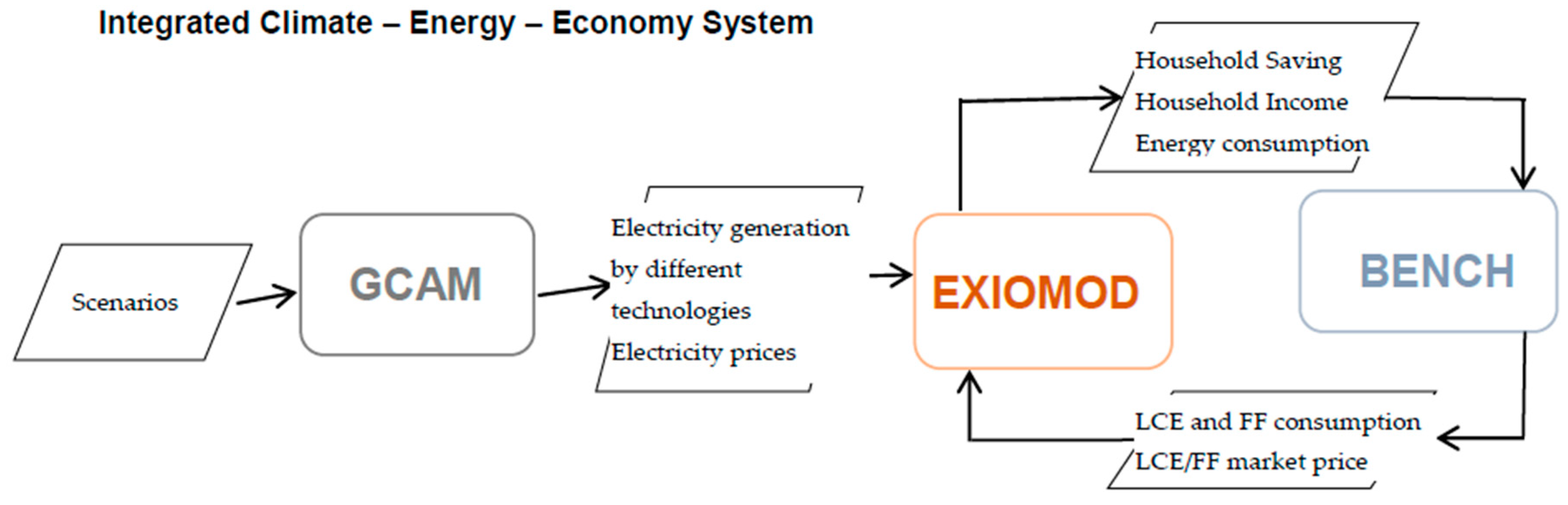
Figure 3 shows the conceptual design of the integrated climate-energy-economy system that is further explained in this section.
3.1. Linking IAM and CGE: GCAM and EXIOMOD
The pre-integration assessment identified that by linking GCAM and EXIOMOD we can simulate how climate mitigation policy scenarios affect different sectors of the economy. To decide on the direction of data flow we considered the following information about the models:
For GCAM, population and GDP are exogenous variables, which are to be provided from external data sources, such as the Shared Socioeconomic Pathways scenarios database of IIASA [
46]. For our simulations we followed the SSP2 storyline, also called Middle of the Road approach since it lies in between the Low challenging scenarios of SSP1 and High challenging scenarios of SSP3 and also between Mitigation challenges dominated SSP5 and Adaptation challenge dominated SSP4 [
47]. It assumes that trends of the recent decades will continue, with some progress towards achieving development goals, reducing resource and energy intensity at historic rates, and slowly decreasing fossil fuel dependency. In our case, even though EXIOMOD can provide GDP predictions we decided that, in order to align the simulations with the IPCC scenarios, it would be convenient to follow the SSP2 approach. Accordingly, we decided to use the assumptions of the SSP2 scenario in both models. Due to the implementation of SSP2 scenarios, the data flow from EXIOMOD to GCAM is not a priority to explore.
For EXIOMOD, GDP and population values are also based on the SSP2 scenario. Total factor productivity is used from the Econmap projections Fouré et al. [
48] because it is provided at country level and per year until 2050. Electricity generation mix is an exogenous variable. For the base year this variable is set using data from the EXIOBASE database. To run scenarios in EXIOMOD we should make assumptions about how this variable can change, depending on management decisions or policies that we model. In practice, if a target value for electricity mix is set at some point in the future, we would need to interpolate between the current EXIOBASE value and the target value. The interpolation is required because EXIOMOD runs on annual basis and needs electricity mix inputs for each run. The interpolation is usually based either on the outcomes of a more specialized energy model, or on the consensus opinion of energy policy experts. On the other hand, GCAM is a specialized energy model, which represents energy technologies and markets very well. GCAM computes energy mix using the capacity and lifetime of technologies, among other parameters. Using the energy mix from GCAM is less ad-hoc and takes technical restrictions into account. Also, GCAM will produce different electricity generation mixes for different scenarios, which is not done when we use EXIOMOD as a stand-alone system. Besides, due to detailed data on costs of electricity generation technologies, GCAM can make a better prediction of changes in electricity prices when we shift to more expensive technologies (renewables).
Based on this, the data flow between the two models should be unidirectional and go from GCAM to EXIOMOD. Apart from electricity prices, there are other variables from GCAM (output) that can be used in EXIOMOD, such as carbon emissions, final energy, primary energy, refinery inputs, floor space, km of passenger transportation and price for food demand. However, for now we have decided to focus only on prices and electricity mix.
After identifying the variables involved in the data exchange between the two models we also found out that the two models represent the data differently. The units used by the two models are shown in
Table 2. The data produced by GCAM should be mediated before they are passed to EXIOMOD, which requires conversion both in units and spatial scales.
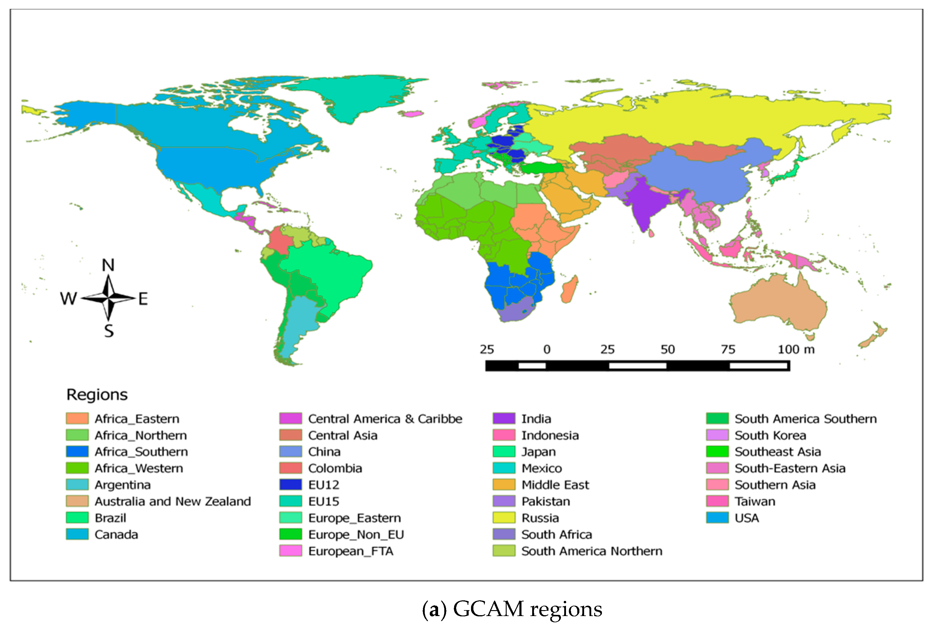
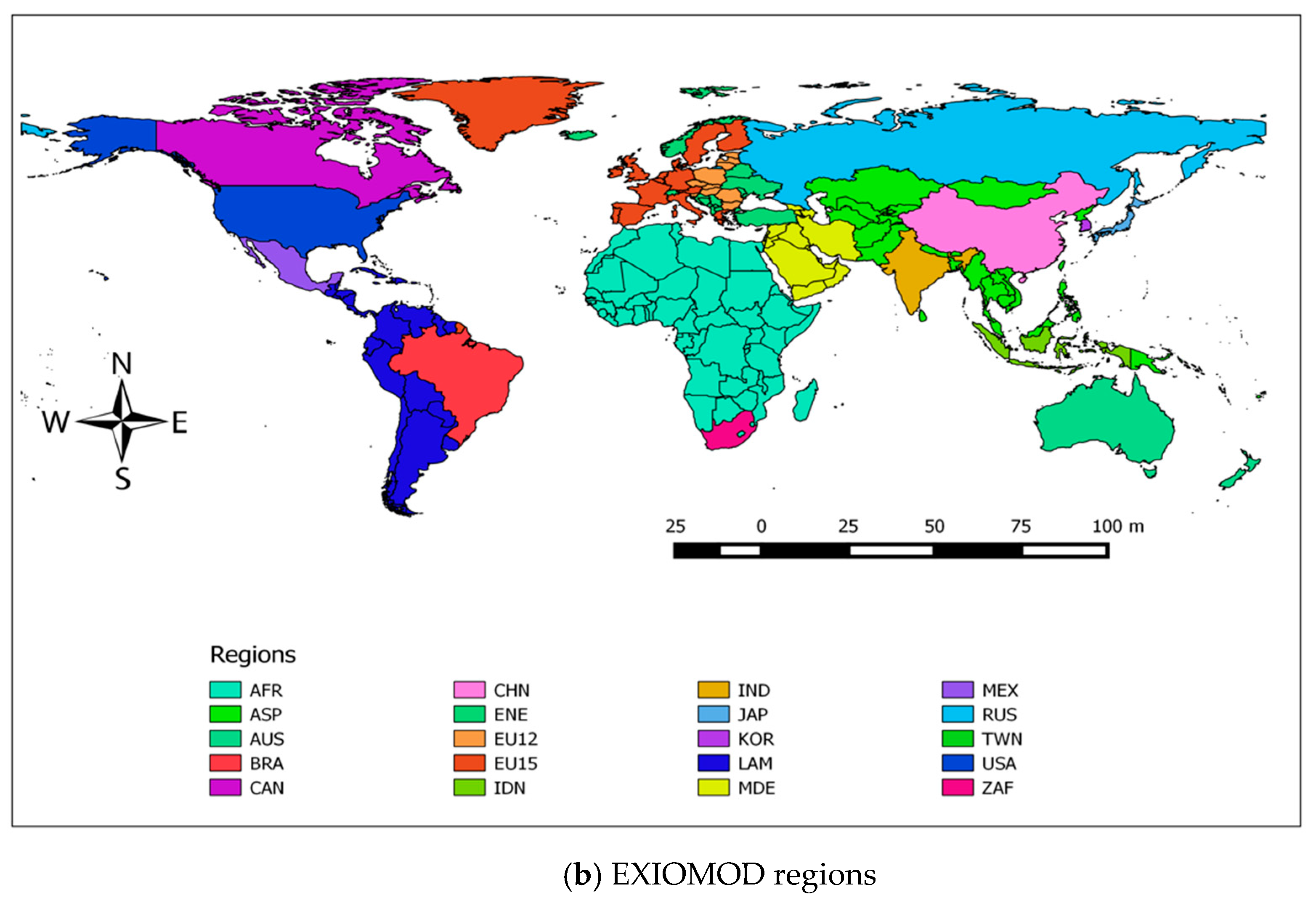
As mentioned earlier, GCAM uses 32 regions/countries to represent the world while EXIOMOD represent the world as 44 regions/countries. With this setting, the data mediation requires direct matching, aggregation, and disaggregation of data between regions/countries of the two models. We found that the data disaggregation process requires additional information, which was not available at hand. To avoid the need for additional data, the regionalization of EXIOMOD was modified from 44 regions to 20 regions (
Figure 4). The regionalization has been chosen in such a way that the resulting 20 regions of EXIOMOD are either equal or more aggregated than the regions in GCAM. The process of regional aggregation of EXIOMOD is relatively straightforward. Firstly, the data on economic transactions and environmental extensions can be just added up, based on the concordance map between the 44 and 20 regions, cancelling out the trade relationships between the regions that get merged. Secondly, the parameters of the models are recalibrated using the standard EXIOMOD formulas based on the aggregated database. This helped us to restrict the spatial aspect of data mediation task to direct matching and aggregation.
The next step was to define how the data for the two selected variables would be mediated. For the electricity generation by different technologies (Et), the data conversion begins with mapping of data between regions of the two models. For aggregated regions data aggregation was done by summing of values. Moreover, Et data include electricity generated using various technologies, such as biomass, wind, coal, gas, hydro, oil, geothermal, refined liquids, and solar. GCAM expresses this data in terms of Exa-Joules (EJ), while EXIOMOD represents it in terms of percentage of each category. Due to this, we compute the share of electricity produced by a certain category as a quotient of amount of energy produced by that category divided by the total amount of energy produced from all categories.
With regards to electricity prices (Ep), GCAM measures them in 1975 USD/GJ, and in EXIOMOD it is measured in relative prices, with the price in the base year taken as 1. The data mediation of Ep from GCAM to EXIOMOD is done using the following steps. For regions that exist in both models the first step is to match the data directly. For regions that do not match directly data are aggregated: weighted average is used to aggregate Ep data with electricity generation in EJ is used as weights. This will give Ep values for all regions of EXIOMOD in 1975 USD/GJ. Then, the next step is to find the relative price for each region. The relative price for a given region is computed by dividing the regional price value for that specific year by the price value of the base year (note that the relative price for the base year is 1).
3.2. Linking CGE and ABM: EXIOMOD and BENCH
The aim of the BENCH–EXIOMOD integration is twofold. Firstly, it provides direct feedbacks between individual behavioral changes, regional changes in market shares of LC vs. FF and impacts of these on other sectors of economy (ABM=>CGE). Secondly, it traces non-residential electricity demand and changes in household incomes as economy evolves (CGE=>ABM). First, at the initialization step, BENCH receives EXIOMOD data on incomes and saving which are consistent with the GDP of the SSP2 scenario implemented in EXIOMOD and GCAM. Information of energy consumption of households and share of LC vs. FF energy production also comes from the interaction between GCAM and EXIOMOD, ensuring the consistency of the modelling exercise. Further, EXIOMOD is updated with the new shares and prices (LC vs. FF) after the market clears and price expectations are updated in BENCH. When EXIOMOD runs and produces new sectoral impacts, the information on income, savings and energy consumption of households is sent to BENCH. Therefore, the linking of EXIOMOD to BENCH assumes a bi-directional data exchange.
Currently both models operate on yearly time steps. Spatially, BENCH is designed to function at the province level: Overijssel province in Netherlands and Navarra region in Spain were chosen. In EXIOMOD these two regions are treated as part of the corresponding hosting countries. To link the two models, the following assumptions are made:
Household income, saving, and energy consumption data generated by EXIOMOD at the national level, in five quantile groups, should be disaggregated to the province level so that it can be used as inputs by BENCH. To do this, we assume that income distribution (level of income within each of the five income quintile groups), saving rates (share of income that goes to savings) and share of income that households in each income quintile spend on electricity are identical in Overijssel and the Netherlands, and in Navarra and Spain. Due to the small size and relatively high homogeneity of incomes in the country, we believe that in the case of the Netherlands this assumption is quite realistic. In the case of Navarra and Spain, however, this assumption could be biased due to relatively small size of the region compared to the whole country. Subject to data availability, one could also use the actual distribution of income classes in the future, especially when considering the cases of more heterogeneous regions.
BENCH calculates the share of low-carbon and fossil fuel energy consumption and new LC and FF energy prices data at provincial level, which we have to up-scale to the country level data so that it will be used by EXIOMOD. Here also we assume that the share of low-carbon and fossil fuel energy consumption at national level is the same as at the province level.
However, if we have household income, saving, and energy consumption data at province level, then data disaggregation should be done to mediate country level data to province level instead of making assumptions. Besides, these assumptions may not work for countries of larger size and higher income inequality than the Netherlands.
At the same time, it is important to highlight the lack of interaction between the BENCH and GCAM stemming from the differences in the geographical scales of the two models. The current version of BENCH only covers two provinces of Spain and the Netherlands, while in GCAM these two countries are part of a wider region formed by 15 countries (the EU15). In the case of the iterations between EXIOMOD and BENCH the data exchange between the two models is implemented through a down-scaling/up-scaling procedure, assuming that the agents and regions of BENCH are representative of Spain and the Netherlands (which are single entities in EXIOMOD). However, we consider that this representativeness assumption does not hold for GCAM, i.e., we cannot assume that Spain and the Netherlands are representative of the whole EU15. A possible solution to this could be the disaggregation of the EU15 in GCAM to the country level, in order to be consistent with the linkage EXIOMOD/BENCH. In such a case, the changes in the preferences of the individuals should be transferred directly to GCAM which would produce new outputs for the energy system that would be passed to EXIOMOD.
3.3. Simulating Climate-Energy-Economy
Model integration is an iterative [
49] and incremental process [
50]. As a first iteration, we implemented the one-way communication between GCAM and EXIOMOD to explore the effect of the emission reduction policy scenario on electricity production by technology and the cascading effect of the changes in the electricity mix and price on the different sectors of the economy. This cannot be done using these models as standalone components. Moreover, the bi-directional data exchange between EXIOMOD and BENCH (
Figure 3) can help us to explore if such policy has any effect on household consumption of green and grey electricity. In addition, the linking of these models helps to minimize ad-hoc input-data producing processes, and to model the climate-energy-economy system across different spatial scales.
4. Web Services to Handle the Interaction of Heterogeneous Models
Once the component models are identified we need to decide on the technique and technology needed to couple them. In our case, the models selected for integration were developed using different modeling paradigms, tools and programming languages: C++ (a general-purpose programming language), NetLogo (a special modeling interface for ABM, using its own programming language of the Logo family), and GAMS (a language for mathematical programming and optimization). An interoperability mechanism is needed for these heterogeneous models to talk to each other.
Models developed using different programming tools can interoperate if additional code is provided to set their inputs, run the model, and expose outputs [
10]. A
wrapper is a thin layer of code that enables such passing of input parameters, running the model, and reading its output. Wrappers can be developed using different programming languages, keeping in mind that:
The language used for one wrapper should not predetermine the languages used for wrappers of other models.
The wrapper built for one model should be reusable for linking to different models, not just one.
A wrapper that enables remote access to models (to keep models on different locations) will have a better chance of including more models and data sources into the integrated system. Such wrapper can improve the accessibility and reusability of models for a wider community.
If the wrapper can make metadata of the model available in machine-readable format then online search for models, semantic mediation, and data conversion becomes possible.
One of the solutions, which suited most of the requirements above, was to use web services as the wrapping mechanism. Web services (WS) are modular and dynamic applications that can be described, published, located or invoked over the network independent of the underlying hardware and software platforms [
51]. They provide for automated data exchange between heterogeneous systems, which can be located anywhere on the Internet. Besides, metadata information of models can be made available through service descriptions of WS, which are accessible by search engines. This can improve the discovery and reuse of models significantly.
In the modeling domain WS have been used for a wide range of applications, to make environmental models interoperable [
52], to integrate ecological forecasting models [
53], to link hydrological models with climate models [
54], to build large scale multi-agent simulations [
55].
The WS approach seemed to be most appropriate to develop wrappers for the models selected above. The wrapper for GCAM was developed on top of the DLL file of the model as a C#-based web service that manipulates GCAM. The wrapper has also functions that can update input XML files and that fetch output data from the database. Similarly, the wrapper for EXIOMOD was built on top of GAMS.NET API. The API runs GAMS-based models (i.e., GAMSJob), and can customize GAMS settings (i.e., GAMSOptions). The wrapper web service consists of a group of functions designed to set the inputs for the simulations, run the model and query the outputs of the simulations. The wrapper web service for BENCH is developed using Java. This is because NetLogo provides a Java-based library file (NetLogo.jar), and using this library the wrapper web service can manipulate the underlying model. These wrappers can be used to run the models as stand-alone WS-based models and also to establish automated data exchange between them.
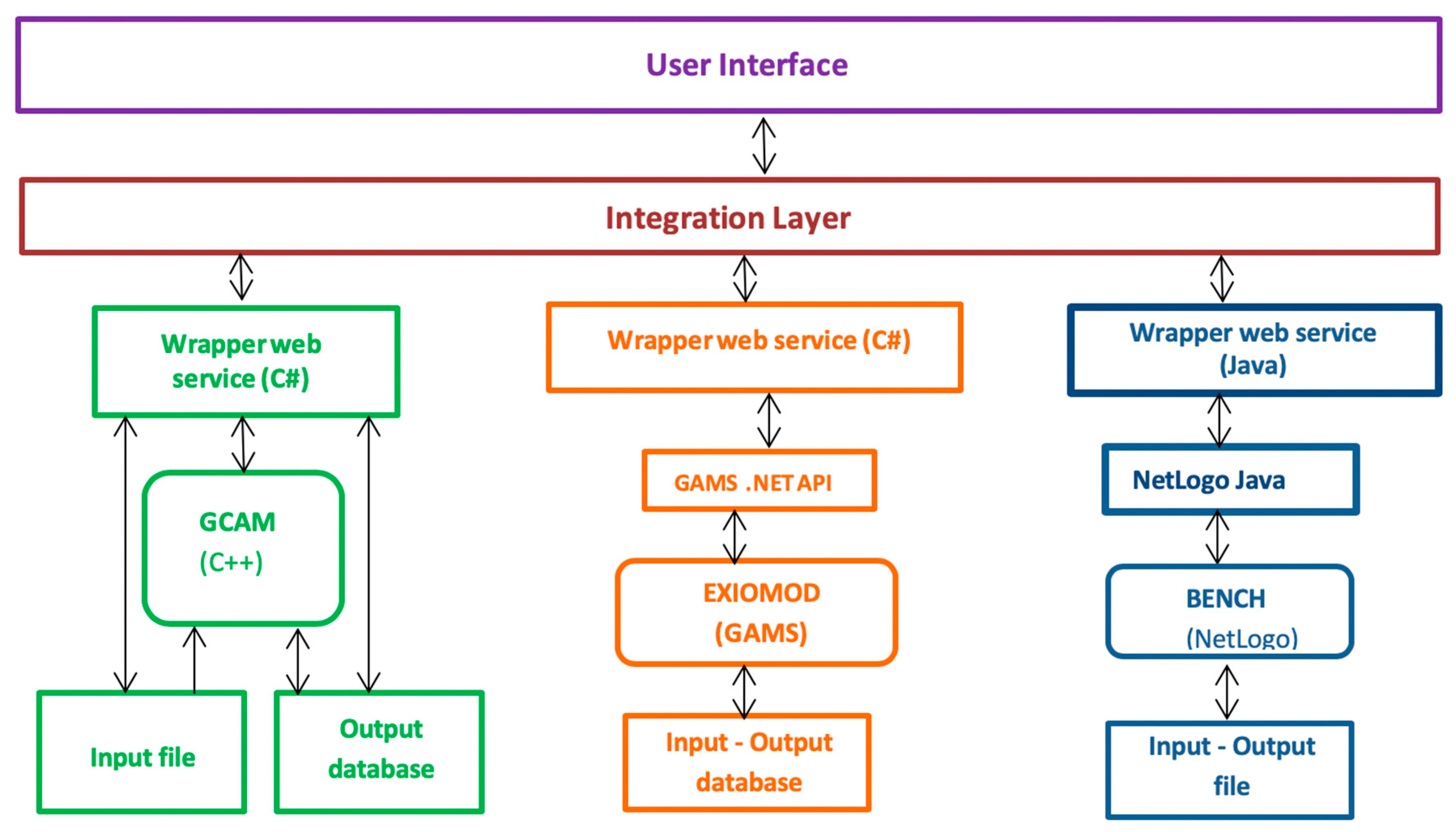
On top of the wrapper WS, an integration layer (
Figure 5) was developed to manipulate the WS-based models. The semantic mediation and dataset conversion functionalities are also built as part of this integration layer. Users can interact with the system using a web-based user interface, which can be accessed from the project website (
http://130.89.221.193:88/dmif/mainpage.aspx) [
56]. The three wrapped models and the integrated system can be accessed from any computer connected to the Internet using a standard browser without the need for installing any of the underlying modeling platforms.
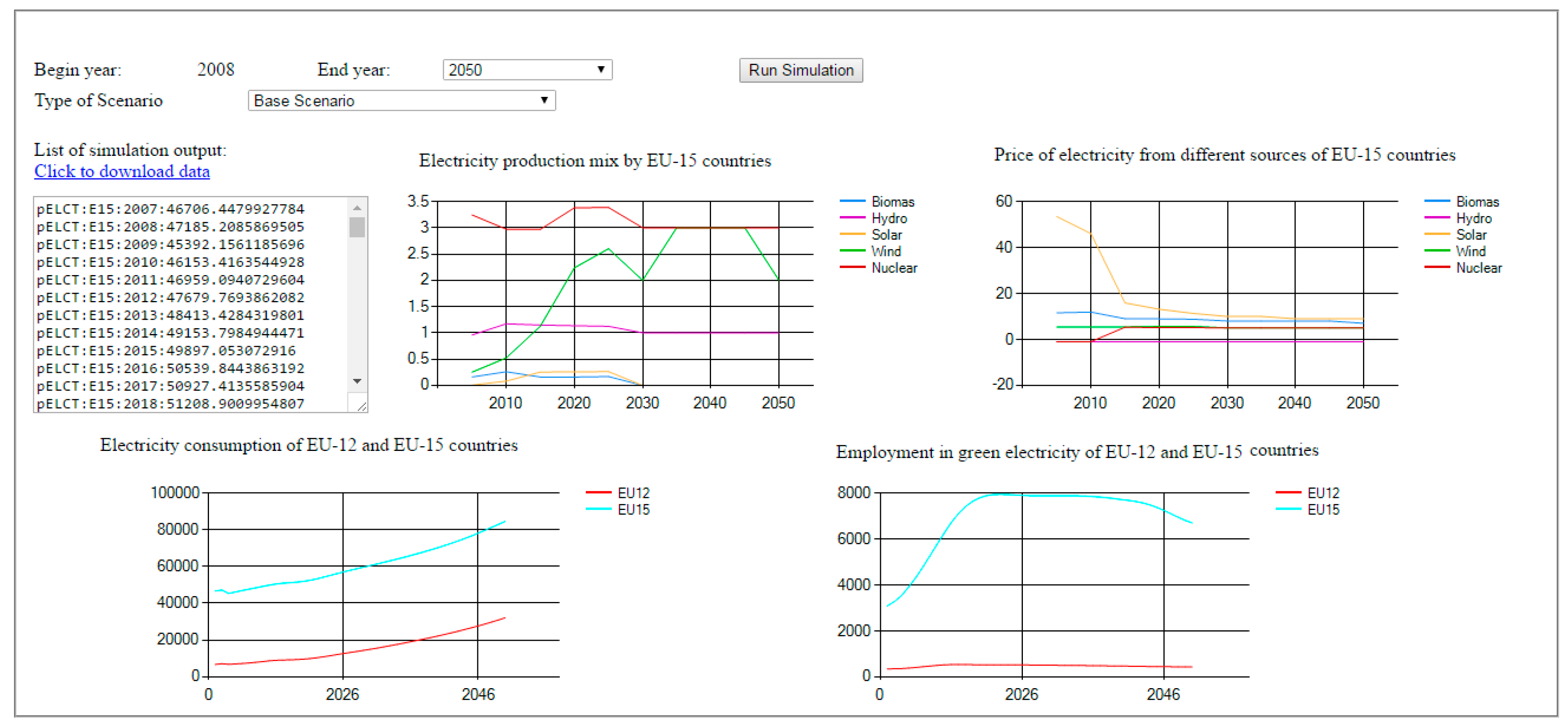
As shown in
Figure 6, the user can select the simulation end year (between 2008 and 2050), the type of scenario and, then, run the simulation. During simulation, the communication between models is orchestrated as follows. GCAM runs the simulation with a time-step of five years until the year 2050. It produces output every five years, i.e., for 2010, 2015, etc. EXIOMOD reads input data both from its database and from the output of GCAM, and it produces a simulation output for every year, i.e., starting from year 2008 until 2050. Since the communication between EXIOMOD and BENCH is bi-directional, at the end of each simulation period the models exchange data. Some simulation outputs from the models are displayed in the graphical user interface and the user can also download them. The complete model output can be accessed from the output files of the corresponding models.
5. Results and Discussion
As a proof of concept, we present the results of an implementation of two global level scenarios for GCAM and simulate them using the integrated framework. The first scenario is a business as usual (base scenario), in which GDP and population values are set using the SSP2 scenario and no specific climate policy is enforced in the system. The second scenario assumes that, on top of the baseline scenario, from 2020 onwards, an emission reduction policy is implemented in the system (policy scenario). The mitigation targets are reported in (
Table 3) and are based on the Intended Nationally Determined Contributions of the Paris Agreement [
38] (
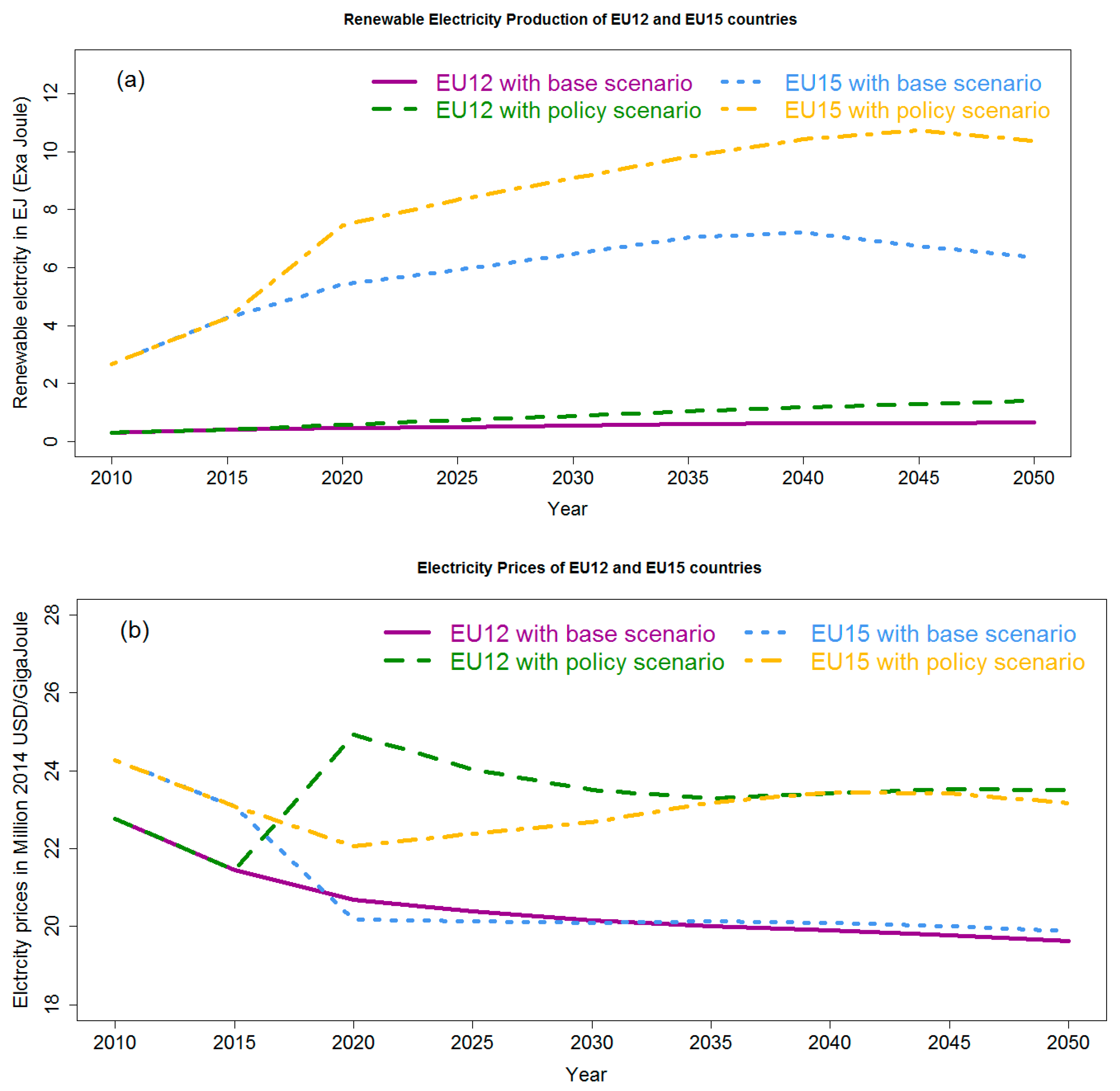
Table 3). For simplicity, we just show the results for the 2 EU regions represented in GCAM: the EU12 (Romania, Bulgaria, Cyprus, Czech Republic, Estonia, Hungary, Lithuania, Latvia, Malta, Poland, Slovakia, Slovenia) and the EU15 (Austria, Belgium, Germany, Denmark, Spain, Finland, France, United Kingdom of Great Britain and Northern Ireland, Greece, Ireland, Italy, Luxembourg, Netherlands, Portugal, Sweden).
The first spot to track the effect of the implemented scenario is at the interface between models, when data is passed from one model to the next one. In particular, the electricity production by technology (E
t) and the price of electricity (E
p) are the two variables passed from GCAM to EXIOMOD.
Figure 7 shows the evolution of renewable electricity production, which is a subset of E
t (
Figure 7a), and E
p (
Figure 7b) for the of EU12 and EU15 countries, in the base and policy scenarios. The results show an increase in both renewable electricity production and E
p in the policy scenario with respect the base. The increase in prices of electricity is associated with the higher costs of the electricity system driven by the increase in the price of CO
2 emission permits affecting to fossil-fueled technologies, and the penetration of renewable technologies.
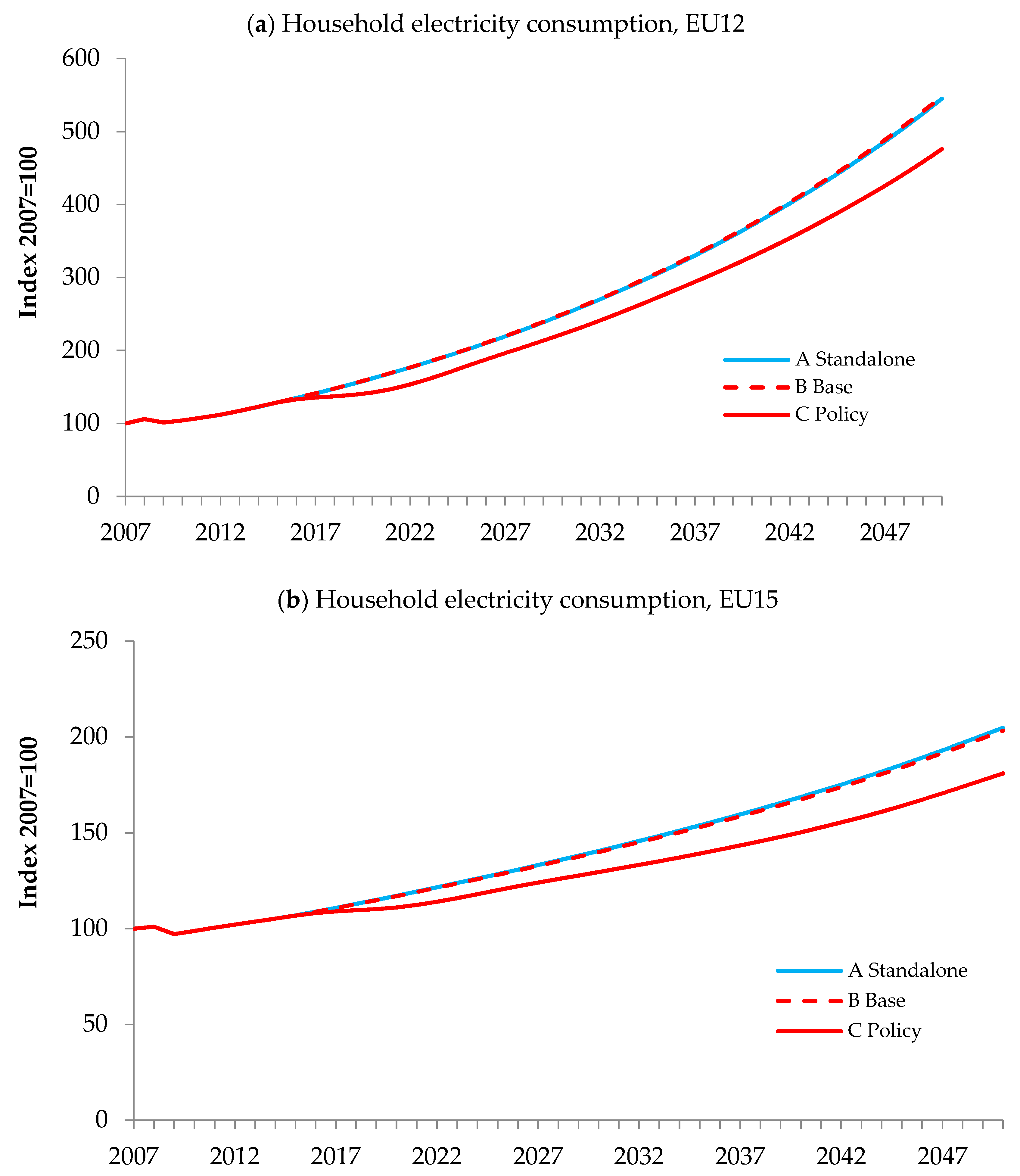
At the end of the simulation the integrated system produces data for hundreds of variables representing different sectors. To demonstrate the effect of the climate policy policies, we select three variables from EXIOMOD: household consumption of electricity, employment in green electricity sector, and import of mining products (including oil and gas). Besides, for comparison we perform the simulations for three different simulation experiments: (A) when EXIOMOD did not receive data from GCAM and BENCH in the base scenario, (B) when the integrated system runs in the base scenario, and (C) the integrated system runs in the policy scenario. The results of the simulations for the selected variables are presented below.
The trend in household electricity consumption is shown in
Figure 8a,b. Each figure presents three lines: Electricity consumption predicted using the standalone system, i.e., using setup (A); Electricity consumption predicted using experimental settings (B); and Electricity consumption using settings (C). The graphs show that implementing these policy scenarios will result in a reduction of household electricity consumption, which is associated with the increase in electricity prices shown in
Figure 7b.
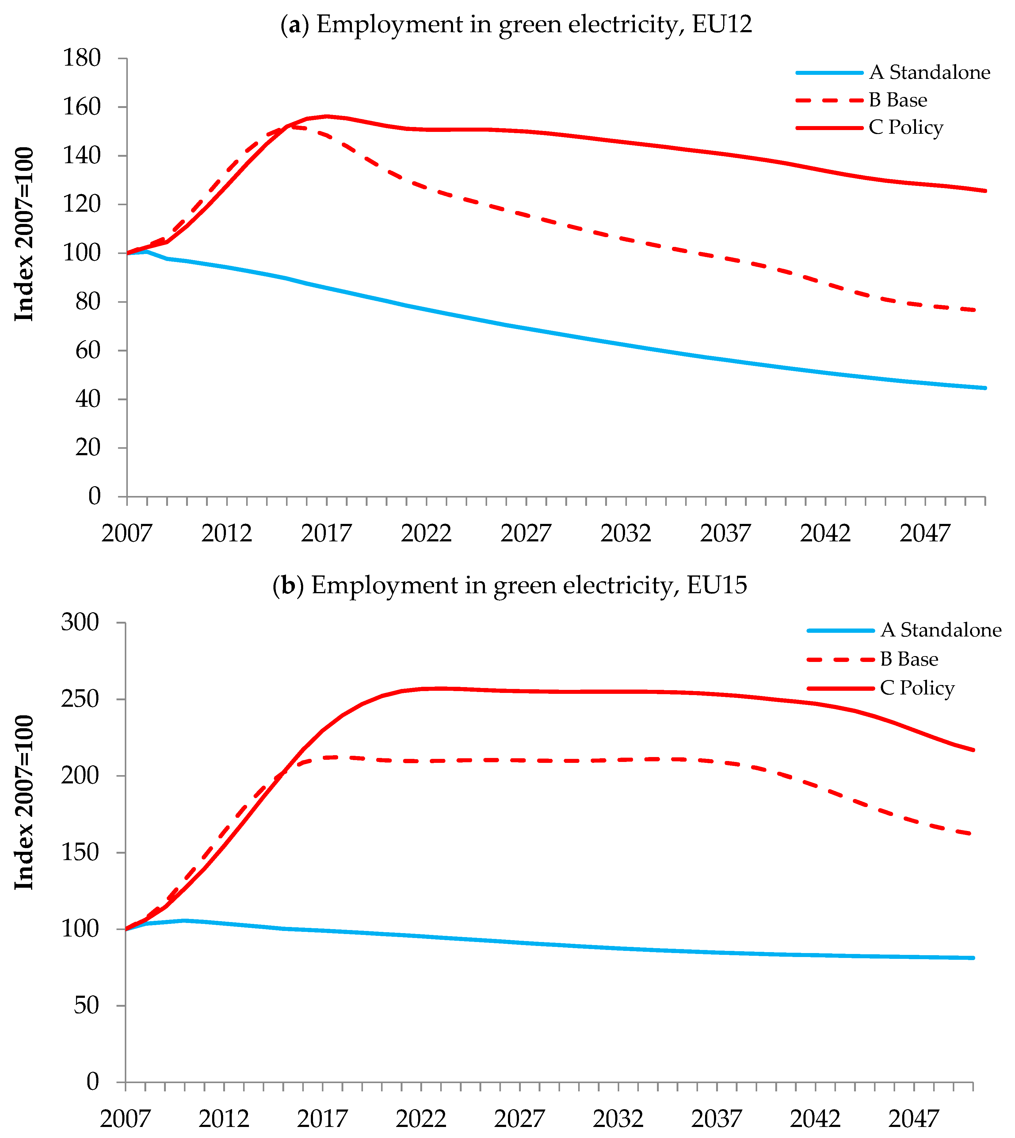
Employment in the green electricity sector is the second variable we selected to illustrate the benefit of building the system-of-systems. As shown in
Figure 9, implementing those emission reduction targets will increase the employment in the green electricity sector, in both EU12 and EU15 countries. This results in consistent with the increase in renewable electricity production (
Figure 7a).
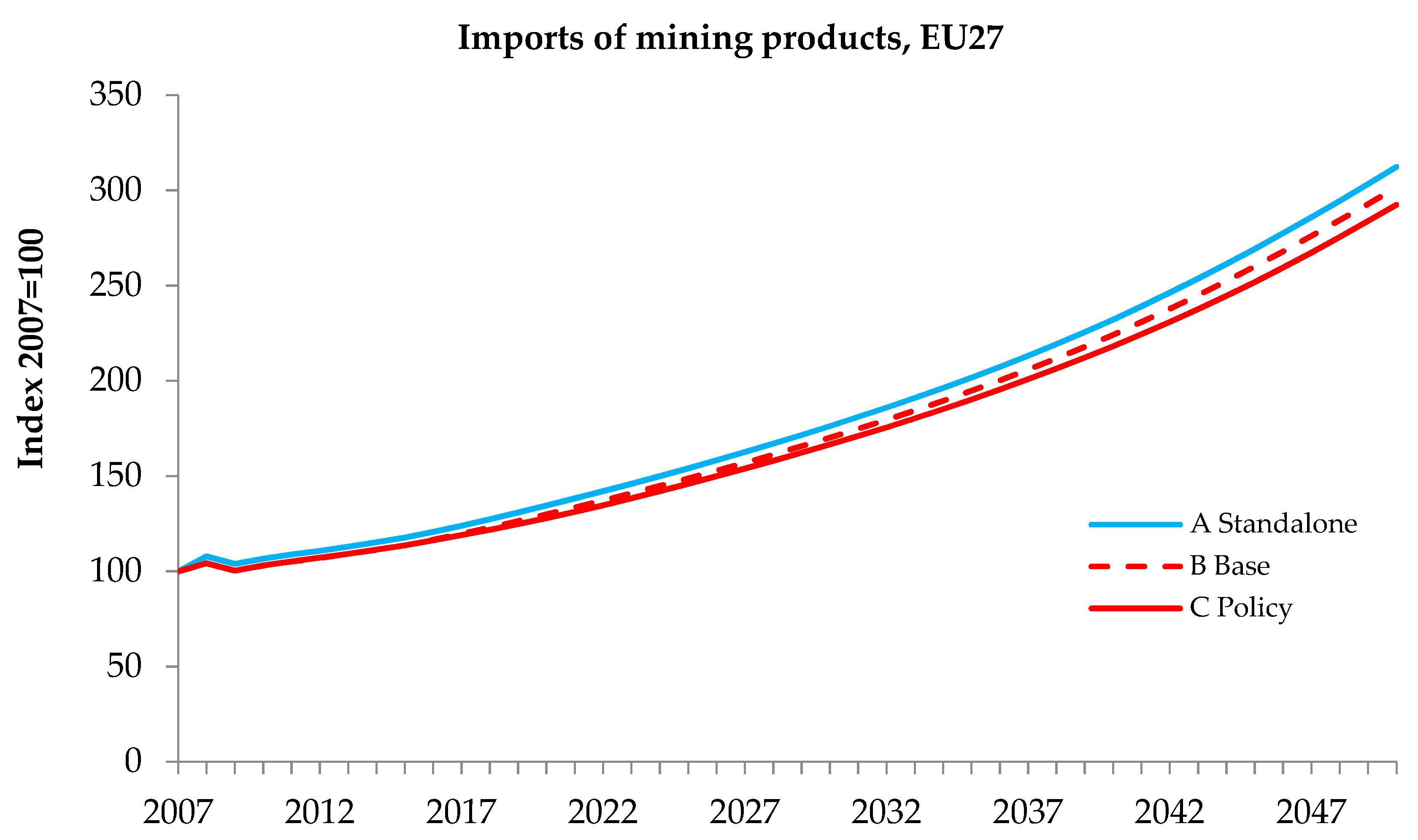
Not all variables show so distinct differences in the three systems analyzed. For example, if we look at the imports of mining products, which includes coal, oil, gas, metals and non-metallic mineral products, in all three systems the results are quite similar (
Figure 10). This is because EXIOMOD does not use a separate variable to represent imports of coal and gas. In the climate policy scenarios there is a substitution of coal power production by natural gas and renewable technologies. The reduction in the imports of coal is to some extent compensated by an increase in the imports of other mining product such as natural gas. In case of policy analysis where coal imports are of particular interest, the choice of model with sufficient level of detail becomes crucial.
In general, linking these standalone models has given us a chance to streamline the ad-hoc input data producing process (i.e., electricity generation mix for EXIOMOD). It also provides the flexibility in implementing targeted scenarios. Impact assessment of climate change policies for specific sectors can be handled using a standalone system, for example, we can use the CGE model to analyze impacts of climate change policy on energy and economics, or on the transportation sector. Model integration allows exploring more complex situations, such as the effect of implemented scenarios across sectors presented in individual standalone models. Each individual model can be set to a number of different system states by setting the various variables to a range of values, and linking such models with other models (which themselves have several system states) will significantly increase the number of system states. For example, in our case the two variables from GCAM (E
t and E
p) can possibly affect all the 163 variables (sectors) of EXIOMOD. Stoorvogel [
16] pointed out that by linking standalone models they could evaluate an ‘infinite number of scenarios’, which we can consider as an important ‘by-product’ of integration.
The integration methodology we described in this paper can be applied in other interdisciplinary studies. The steps we followed in the pre-integration assessment and in conceptualizing the integrated system can be replicated by other similar projects, also for soft-linking of models, which is popular in climate and energy research. We observed that identifying the appropriate models and formulating the interaction between them is difficult and time consuming. This is mainly because models are poorly documented and model owners still have to be engaged to create a common understanding about participating models, which may require several iterations and discussions. We saw that, besides having clearly defined integration objectives, a list of scenarios together with the corresponding indicator variables (to be tested by the integrated system) could help to keep pre-integration assessment discussions focused and productive.
We also found that the technical interoperability aspect of integration could be standardized and reused. In our specific case, wrapping models with web services was the standard for technical interoperability. The web service based wrappers developed to link models can be reused in other cases. The wrappers we developed can be accessed from any platform, and they can also be reused with non-web service based integration frameworks. Besides, wrapper classes developed to encapsulate NetLogo and GAMS based models can be easily customized in wrapping new models. Additional NetLogo or GAMS based models can be incorporated into our system without reinventing the wrappers. It requires only modifying the model name, input-output variable names, and the path in which the base models are residing.
However, our case study demonstrated that semantic mediation and data conversion tasks might require case specific functionalities. For example, if we link GCAM to yet another model then data processing may be different because of different combinations of input-output variables to be exchanged with the new model, different units used in those variables, and the different spatial and temporal scales assumed for them. This is certainly challenging for building generic semantic mediation and data conversion tools. On the other hand, we did see that some generic functionality to handle some parts of semantic mediation and dataset conversion can be built. For example, a standardized unit conversion functionality for the International System of Units and derived units can be provided using available units ontologies. Similarly, automatic re-gridding functionalities in Community Surface Dynamics Modeling System [
10], or Earth System Modeling Framework [
57], are good examples of advances toward standardized data mediation.
There are several advantages of web-based modeling, such as: ease of use and collaboration, simple licensing, deployment, reuse, access control, versioning, customization and maintenance [
58]. On top of this, with the web service based approach we can incorporate new models, modify existing models, or remove a member model without disturbing the existing integrated system. This is because in web service based integration a member component has no knowledge about the existence of the other components. Communication between component models is through the integration layer. This gives us the opportunity to create an extendable model integration platform, which can evolve through time. The downside of the web service based approach is that it requires high-speed Internet access and can be quite slow when large amounts of data are exchanged repeatedly. However, the greater the processing time of the participating models, the less the communication over-head [
59].
Any modeling is accompanied with uncertainty due to approximations used, ignored or misrepresented processes in conceptualization of the model, uncertainties in data, or inability to accurately quantify the input parameters of a model [
60]. Uncertainty is inevitable due to the nature of the task [
61]. Of course, as more models are coupled and the higher the complexity of the overall system of systems we build, the more parameters of the system we have, the higher the overall uncertainty will be. Integration of models is likely to propagate uncertainty throughout the model chain [
53]. There are certain new parameters that come just from the coupling algorithms used. Belete and Voinov [
31] have explored the sensitivity of the model integration to various combinations of time-stepping chosen in component models, as well as to the differences in the functions and the numeric methods assumed. The acceptance of model output, especially in complex systems such as the one we described above will be always contingent upon proper identifying and quantifying the associated uncertainty. In our case this means quantifying uncertainty in the three component models as well as tracking how it will be propagating through the integrated system. However, this requires a separate extensive treatment, which at this point this goes beyond the scope of the paper.
6. Conclusions
There is a growing number of high-quality climate, energy and economy models operating at different scales and generating relevant information to support energy policy decisions. The challenge is, to integrate the existing fragmented models, capitalizing on the strengths and capabilities of individual components. There is a strong movement to find synergies in the existing international knowledge base. Instead of developing new models from scratch each time we are facing a new research problem: how to make existing models transparent and open for reuse? The unprecedented evolution of computational methods makes it possible to dynamically integrate existing climate-energy-economy models and use them in symbiosis, as long as we know what they can offer and how they can complement each other.
This paper contributes to the integration modeling efforts by presenting a novel web-platform and illustrating its functionalities by integrating three very different energy models—IAM, ABM and CGE. The emphasis here is on the integration methodology and the necessary module coupling steps. We demonstrate how we can link models, which operate at different scales from global to household, to function as a system-of-systems. GCAM IAM, the EXIOMOD CGE and the BENCH ABM are used for a step by step illustration of how such integration can be done in practice and how it can be used in other applications. Firstly, the pre-integration process takes place, which leads to some joint decisions about the synergies that various models can generate by feeding information from one model to another and back. Secondly, we illustrate how the detailed data exchange is designed, resolving any potential conflicts in unit measurements, vocabulary and variable overwriting. Lastly, the novel web-platform for model integration is presented with a simple illustrative example in application to climate policy.
Our integration technique is quite general and can accommodate all sorts of data passing between models. If other variables are chosen for data exchange (say, feeding end-use demand into EXIOMOD), it will require the same type of decisions as the ones we describe in
Section 2.1 with little, if any, additional programming. The same technique and architecture can be applied to couple additional component models, again with little programming needed once they are wrapped as web services. By linking the three exemplar models we were able to create a framework that can help to investigate the energy and economy aspects of climate change, which could be hardly accomplished using stand-alone model components. Despite some clear promises of future reuse of the components we have developed in other system-of-systems design and other integration schemes, we saw that there are still big concerns about ‘automating’ and ‘streamlining’ model integration [
28]. It remains very unlikely that productive integration can be achieved without the more qualitative pre-integration assessment process, which requires very active involvement of stakeholders/modelers for scoping the objectives of integration, formulating scenarios, reviewing and identifying the candidate models, and conceptualizing the envisaged system. The pre-integration assessment phase can take a significant portion of the project life-time with a number of iterations needed. Moreover, failing to identify mismatches between models at this stage could result in a big waste of resources and delays to the project. We also demonstrate that web service based approach can be used to link diverse models which are developed using different modeling languages and paradigms. The web service wrappers developed can be reused by other integration frameworks, also by those that are non-service based. Our approach can be applied in other similar projects, which require to link models that operate at different temporal and spatial scales.


 ,
, 


