Assessment of Offshore Wind Characteristics and Wind Energy Potential in Bohai Bay, China


Abstract
1. Introduction
2. Wind Data Analysis Methods
2.1. Weibull Distribution
2.2. Nakagami Distribution
2.3. Rician Distribution
2.4. Rayleigh Distribution
2.5. Coefficient of Determination
3. Wind Data
- (1)
- Spring: March–May;
- (2)
- Summer: June–August;
- (3)
- Autumn: September–November;
- (4)
- Winter: December–February.
4. Results and Discussion
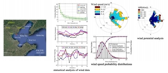
4.1. Statistical Analysis of Wind Data
4.2. Wind Speed Probability Distributions
4.3. Wind Potential Analysis at Bohai Bay
4.4. Evaluation of the Probability Density Functions
5. Conclusions
- In Bohai Bay, the wind mainly blows from the east (E −15°–45°), followed by the southeast (SE −55°–−45°) and northeast (NE 55°–75°). The winds speed in Bohai Bay is mostly lower than 12 m/s, generally in the range of 4–8 m/s, and the main wind speed ranges in April and October are higher than those in August and December. However, in summer, the magnitude of average wind speeds is lower but the magnitude of extreme wind speeds is higher due to the occurrence of monsoons, such as typhoons. The wind speed from 20:00 to 08:00 is higher than that from 08:00 to 20:00 and exhibits a sinusoidal pattern over each hour of each day. The turbulence intensity is low due to the low surface roughness and mainly depends on wind speeds instead of periods.
- Weibull, Nakagami, Rician, and Rayleigh distributions all performed well in comparison to the observed wind speed, where Nakagami and Rician distributions were first introduced in the field of wind energy and performed well in predicting the wind speed distributions. However, none of the distributions fit the wind speed distributions in August due to the high percentage of null winds.
- The most probable wind speed, the most energy-carrying wind speed, and the wind power density based on Nakagami (Rician) distributions were first proposed and used to assess the wind potential and forecast the wind characteristics in Bohai Bay. Nakagami distribution performed better than the other three distributions in forecasting WPD. Based on the results of the analysis, Bohai Bay can be considered as a wind class I region, with east as the dominant direction as the corresponding WPD is mostly below 200 W/m2 and mainly faces the east.
Author Contributions
Funding
Acknowledgments
Conflicts of Interest
Notations and Abbreviations
| Probability density function | |
| R2 | Correlation coefficient |
| FPSO | Floating production storage and offloading |
| k | Weibull shape parameter |
| Nakagami shape parameter | |
| Gamma function | |
| Rician scale parameter | |
| The modified Bessel function of the first-kind with an order of | |
| Rayleigh scale parameter (m/s) | |
| Nak | Nakagami |
| Ric | Rician |
| WSR | Wind speed range |
| SD | Standard deviation |
| Most energy-carrying wind speed | |
| WED | Wind energy density (kWh/m2) |
| TI | Turbulence intensity |
| CDF | Cumulative distribution function |
| RMSE | Root mean square error |
| Air density (kg/m3) | |
| c | Weibull scale parameter (m/s) |
| Nakagami scale parameter | |
| Upper incomplete gamma function | |
| Rician location parameter | |
| Marcum Q-function | |
| v | Wind speed (m/s) |
| Wei | Weibull |
| Ray | Rayleigh |
| MWS | Mean wind speed |
| The most probable wind speed | |
| WPD | Wind speed density (W/m2) |
| T | Time period |
| MTI | Mean turbulence intensity |
References
- Global Wind Energy Council. Global Wind Energy Report: Annual Market Update 2017; Global Wind Energy Council: Bruxelles, Belgium, 2018. [Google Scholar]
- Zhao, X.; Ren, L. Focus on the development of offshore wind power in China: Has the golden period come? Renew. Energy 2015, 81, 644–657. [Google Scholar] [CrossRef]
- Niu, T.; Wang, J.; Lu, H.; Du, P. Uncertainty modeling for chaotic time series based on optimal multi-input multi-output architecture: Application to offshore wind speed. Energy Convers. Manag. 2018, 156, 597–617. [Google Scholar] [CrossRef]
- Ali, S.; Lee, S.M.; Jang, C.M. Statistical analysis of wind characteristics using Weibull and Rayleigh distributions in Deokjeok-do Island–Incheon, South Korea. Renew. Energy 2018, 123, 652–663. [Google Scholar] [CrossRef]
- Lun, I.Y.F.; Lam, J.C. A study of Weibull parameters using long-term wind observations. Renew. Energy 2000, 20, 145–153. [Google Scholar] [CrossRef]
- Baseer, M.A.; Meyer, J.P.; Rehman, S.; Alam, M.M. Wind power characteristics of seven data collection sites in Jubail, Saudi Arabia using Weibull parameters. Renew. Energy 2017, 102, 35–49. [Google Scholar] [CrossRef]
- Rodriguez-Hernandez, O.; Jaramillo, O.A.; Andaverde, J.A.; del Río, J.A. Analysis about sampling, uncertainties and selection of a reliable probabilistic model of wind speed data used on resource assessment. Renew. Energy 2013, 50, 244–252. [Google Scholar] [CrossRef]
- Wais, P. Two and three-parameter Weibull distribution in available wind power analysis. Renew. Energy 2017, 103, 15–29. [Google Scholar] [CrossRef]
- Seguro, J.V.; Lambert, T.W. Modern estimation of the parameters of the Weibull wind speed distribution for wind energy analysis. J. Wind Eng. Ind. Aerodyn. 2000, 85, 75–84. [Google Scholar] [CrossRef]
- Zheng, C.W.; Li, C.Y.; Pan, J.; Liu, M.Y.; Xia, L.L. An overview of global ocean wind energy resource evaluations. Renew. Sustain. Energy Rev. 2016, 53, 1240–1251. [Google Scholar] [CrossRef]
- Shu, Z.R.; Li, Q.S.; Chan, P.W. Statistical analysis of wind characteristics and wind energy potential in Hong Kong. Energy Convers. Manag. 2015, 101, 644–657. [Google Scholar] [CrossRef]
- Gao, X.; Yang, H.; Lu, L. Study on offshore wind power potential and wind farm optimization in Hong Kong. Appl. Energy 2014, 130, 519–531. [Google Scholar] [CrossRef]
- Wang, J.; Qin, S.; Jin, S.; Wu, J. Estimation methods review and analysis of offshore extreme wind speeds and wind energy resources. Renew. Sustain. Energy Rev. 2015, 42, 26–42. [Google Scholar] [CrossRef]
- Zhang, H.; Yu, Y.J.; Liu, Z.Y. Study on the Maximum Entropy Principle applied to the annual wind speed probability distribution: A case study for observations of intertidal zone anemometer towers of Rudong in East China Sea. Appl. Energy 2014, 114, 931–938. [Google Scholar] [CrossRef]
- Chang, R.; Zhu, R.; Badger, M.; Hasager, C.B.; Xing, X.; Jiang, Y. Offshore wind resources assessment from multiple satellite data and WRF modeling over South China Sea. Remote Sens. 2015, 7, 467–487. [Google Scholar] [CrossRef]
- Wan, Y.; Fan, C.; Dai, Y.; Li, L.; Sun, W.; Zhou, P.; Qu, X. Assessment of the joint development potential of wave and wind energy in the South China Sea. Energies 2018, 11, 398. [Google Scholar] [CrossRef]
- Ouarda, T.B.M.J.; Charron, C.; Shin, J.Y.; Marpu, P.R.; Al-Mandoos, A.H.; Al-Tamimi, M.H.; Ghedira, H.; Al Hosaryc, T.N. Probability distributions of wind speed in the UAE. Energy Convers. Manag. 2015, 93, 414–434. [Google Scholar] [CrossRef]
- Akgül, F.G.; Şenoğlu, B.; Arslan, T. An alternative distribution to Weibull for modeling the wind speed data: Inverse Weibull distribution. Energy Convers. Manag. 2016, 114, 234–240. [Google Scholar] [CrossRef]
- Mohammadi, K.; Alavi, O.; Mostafaeipour, A.; Goudarzi, N.; Jalilvan, M. Assessing different parameters estimation methods of Weibull distribution to compute wind power density. Energy Convers. Manag. 2016, 108, 322–335. [Google Scholar] [CrossRef]
- Hennessey, J.P., Jr. Some aspects of wind power statistics. J. Appl. Meteorol. 1977, 16, 119–128. [Google Scholar] [CrossRef]
- Deaves, D.M.; Lines, I.G. On the fitting of low mean windspeed data to the Weibull distribution. J. Wind Eng. Ind. Aerodyn. 1997, 66, 169–178. [Google Scholar] [CrossRef]
- Kumar, M.B.H.; Balasubramaniyan, S.; Padmanaban, S.; Holm-Nielsen, J.B. Wind Energy Potential Assessment by Weibull Parameter Estimation Using Multiverse Optimization Method: A Case Study of Tirumala Region in India. Energies 2019, 12, 2158. [Google Scholar] [CrossRef]
- Carta, J.A.; Ramirez, P.; Velazquez, S. A review of wind speed probability distributions used in wind energy analysis: Case studies in the Canary Islands. Renew. Sustain. Energy Rev. 2009, 13, 933–955. [Google Scholar] [CrossRef]
- Chang, T.P. Estimation of wind energy potential using different probability density functions. Appl. Energy 2011, 88, 1848–1856. [Google Scholar] [CrossRef]
- Jiang, H.; Wang, J.; Wu, J.; Geng, W. Comparison of numerical methods and metaheuristic optimization algorithms for estimating parameters for wind energy potential assessment in low wind regions. Renew. Sustain. Energy Rev. 2017, 69, 1199–1217. [Google Scholar] [CrossRef]
- Nakagami, M. The m-distribution—A general formula of intensity distribution of rapid fading. Proceedings of a Symposium Held at the University of California, Los Angeles, CA, USA, 18–20 June 1958; pp. 3–36. [Google Scholar]
- de Queiroz, W.J.L.; de Almeida, D.B.T.; Madeiro, F.; Lopes, W.T.A. Signal-to-noise ratio estimation for M-QAM signals in η−μ and κ−μ fading channels. EURASIP J. Adv. Signal Process. 2019, 2019, 20. [Google Scholar] [CrossRef]
- Odeyemi, K.O.; Owolawi, P.A. Selection combining hybrid FSO/RF systems over generalized induced-fading channels. Opt. Commun. 2019, 433, 159–167. [Google Scholar] [CrossRef]
- Marie-Helene, R.C.; Francois, D.; Gilles, S.; Guy, C. Assessment of carotid artery plaque components with machine learning classification using homodyned-K parametric maps and elastograms. IEEE Trans. Ultrason. Ferroelectr. Freq. Control 2018. [Google Scholar] [CrossRef]
- Rice, S.O. Mathematical Analysis of Random Noise. Bell Syst. Tech. J. 1945, 23–24. [Google Scholar] [CrossRef]
- Le Khoa, N. A review of selection combining receivers over correlated Rician fading. Digit. Signal Process. 2019, 83, 1–22. [Google Scholar]
- Leung, D.Y.C.; Yang, Y. Wind energy development and its environmental impact: A review. Renew. Sustain. Energy Rev. 2012, 16, 1031–1039. [Google Scholar] [CrossRef]
- Turbines—Part, W. 12-1: Power Performance Measurements of Electricity Producing Wind Turbines; American National Standards Institute: Washington, DC, USA, 2005.
- Hansen, K.S.; Barthelmie, R.J.; Jensen, L.E.; Sommer, A. The impact of turbulence intensity and atmospheric stability on power deficits due to wind turbine wakes at Horns Rev wind farm. Wind Energy 2012, 15, 183–196. [Google Scholar] [CrossRef]
- Barthelmie, R.J.; Hansen, K.S.; Pryor, S.C. Meteorological Controls on Wind Turbine Wakes. Proc. IEEE 2013, 101, 1010–1019. [Google Scholar] [CrossRef]
- Jamil, M.; Parsa, S.; Majidi, M. Wind power statistics and an evaluation of wind energy density. Renew. Energy 1995, 6, 623–628. [Google Scholar] [CrossRef]
- Celik, A.N. A statistical analysis of wind power density based on the Weibull and Rayleigh models at the southern region of Turkey. Renew. Energy 2004, 29, 593–604. [Google Scholar] [CrossRef]
- Zheng, C.; Pan, J.; Li, J. Assessing the China Sea wind energy and wave energy resources from 1988 to 2009. Ocean Eng. 2013, 65, 39–48. [Google Scholar] [CrossRef]
- Oh, K.Y.; Kim, J.Y.; Lee, J.K.; Ryu, M.S.; Lee, J.S. An assessment of wind energy potential at the demonstration offshore wind farm in Korea. Energy 2012, 46, 555–563. [Google Scholar] [CrossRef]
- Elliott, D.L.; Holladay, C.G.; Barchet, W.R.; Foote, H.P.; Sandusky, W.F. Wind Energy Resource Atlas of the United States; Pacific Northwest Lab.: Richland, WA, USA, 1987. [Google Scholar]


| Location | Latitude | Longitude | Begin | End | Height (m) | Interval | Recovery Rate |
|---|---|---|---|---|---|---|---|
| Bohai Bay | 38.7° N | 118.7° E | 2015.03 | 2017.05 | 60 | 1 s | 96% |
| WSR (m/s) | Percentage of Total Wind Occurrence (%) | |||||
|---|---|---|---|---|---|---|
| Spring | Summer | Autumn | Winter | Annual | Sum | |
| [0,1) | 0.81 | 3.43 | 1.48 | 1.53 | 1.82 | 1.82 |
| [1,2) | 2.30 | 5.10 | 4.59 | 5.43 | 4.38 | 6.20 |
| [2,3) | 5.46 | 12.65 | 11.23 | 11.99 | 10.39 | 16.59 |
| [3,4) | 7.95 | 16.66 | 13.77 | 14.14 | 13.19 | 29.78 |
| [4,5) | 11.77 | 17.92 | 14.15 | 14.73 | 14.27 | 44.45 |
| [5,6) | 15.15 | 15.20 | 13.62 | 13.15 | 12.54 | 58.72 |
| [6,7) | 16.29 | 11.60 | 11.46 | 10.99 | 10.71 | 71.26 |
| [7,8) | 16.21 | 8.26 | 9.65 | 8.98 | 6.64 | 81.97 |
| [8,9) | 10.63 | 4.03 | 6.19 | 5.89 | 4.38 | 88.61 |
| [9,10) | 7.09 | 2.15 | 4.37 | 4.03 | 2.70 | 92.99 |
| [10,11) | 3.72 | 1.25 | 3.06 | 2.80 | 1.59 | 95.69 |
| [11,12) | 1.59 | 0.78 | 2.05 | 1.95 | 1.04 | 97.28 |
| [12,13) | 0.67 | 0.45 | 1.50 | 1.51 | 0.57 | 98.32 |
| [13,14) | 0.19 | 0.20 | 0.90 | 0.97 | 0.38 | 98.89 |
| [14,15) | 0.09 | 0.12 | 0.62 | 0.69 | 0.27 | 99.27 |
| [15,16) | 0.04 | 0.08 | 0.44 | 0.50 | 0.18 | 99.54 |
| [16,17) | 0.02 | 0.06 | 0.32 | 0.33 | 0.13 | 99.72 |
| [17, ∞) | 0.01 | 0.09 | 0.62 | 0.40 | 0.15 | 100 |
| WRS (m/s) | Percentage of Total Wind Occurrence | |||||||||||
|---|---|---|---|---|---|---|---|---|---|---|---|---|
| Jan | Feb | Mar | Apr | May | Jun | Jul | Aug | Sep | Oct | Nov | Dec | |
| [0,1) | 1.53 | 1.32 | 0.76 | 1.00 | 0.68 | 1.74 | 3.02 | 5.62 | 2.77 | 0.74 | 0.80 | 1.71 |
| [1,2) | 5.59 | 4.14 | 2.31 | 2.30 | 2.29 | 3.25 | 4.86 | 7.23 | 6.93 | 3.11 | 3.55 | 6.41 |
| [2,3) | 12.55 | 9.59 | 6.44 | 4.97 | 5.09 | 6.88 | 12.23 | 18.94 | 15.53 | 8.05 | 9.87 | 13.55 |
| [3,4) | 14.03 | 13.34 | 9.07 | 7.08 | 7.81 | 13.13 | 17.57 | 19.11 | 17.71 | 11.27 | 12.00 | 14.96 |
| [4,5) | 13.89 | 15.22 | 12.34 | 10.26 | 12.64 | 16.02 | 19.95 | 17.38 | 16.83 | 12.24 | 13.20 | 15.12 |
| [5,6) | 12.41 | 14.58 | 16.92 | 13.18 | 15.46 | 15.89 | 16.38 | 13.08 | 14.13 | 13.26 | 13.44 | 12.62 |
| [6,7) | 10.56 | 12.98 | 16.61 | 15.06 | 17.14 | 14.93 | 11.38 | 8.50 | 9.52 | 12.86 | 12.12 | 9.65 |
| [7,8) | 8.84 | 10.29 | 15.53 | 16.52 | 16.51 | 13.02 | 7.52 | 4.37 | 6.61 | 11.79 | 10.73 | 7.96 |
| [8,9) | 5.97 | 6.68 | 9.39 | 11.79 | 10.62 | 7.11 | 3.16 | 1.98 | 3.65 | 7.88 | 7.23 | 5.10 |
| [9,10) | 4.32 | 4.13 | 6.02 | 8.87 | 6.38 | 3.74 | 1.57 | 1.25 | 2.49 | 5.75 | 4.98 | 3.66 |
| [10,11) | 3.13 | 2.50 | 2.70 | 5.17 | 3.27 | 2.18 | 0.73 | 0.94 | 1.80 | 4.09 | 3.34 | 2.73 |
| [11,12) | 2.30 | 1.57 | 1.09 | 2.41 | 1.28 | 1.24 | 0.51 | 0.62 | 1.03 | 2.88 | 2.28 | 1.94 |
| [12,13) | 1.84 | 1.18 | 0.50 | 0.94 | 0.56 | 0.60 | 0.37 | 0.41 | 0.56 | 2.19 | 1.79 | 1.47 |
| [13,14) | 1.17 | 0.75 | 0.19 | 0.24 | 0.16 | 0.16 | 0.21 | 0.24 | 0.24 | 1.33 | 1.19 | 0.95 |
| [14,15) | 0.77 | 0.58 | 0.08 | 0.11 | 0.07 | 0.04 | 0.16 | 0.14 | 0.11 | 0.92 | 0.90 | 0.72 |
| [15,16) | 0.48 | 0.46 | 0.03 | 0.06 | 0.03 | 0.01 | 0.13 | 0.08 | 0.05 | 0.63 | 0.69 | 0.55 |
| [16,17) | 0.29 | 0.32 | 0.01 | 0.03 | 0.01 | 0.01 | 0.10 | 0.05 | 0.02 | 0.43 | 0.54 | 0.39 |
| [17, ∞) | 0.31 | 0.37 | 0.00 | 0.02 | 0.00 | 0.04 | 0.17 | 0.05 | 0.02 | 0.59 | 1.37 | 0.51 |
| Season | Annual | Spring | Summer | Autumn | Winter |
|---|---|---|---|---|---|
| MWS (m/s) | 5.2503 | 5.9326 | 4.4912 | 5.3854 | 5.2428 |
| SD (m/s) | 2.8103 | 2.3761 | 2.3941 | 3.1001 | 3.0694 |
| EWS (m/s) | 36.8 | 26.1 | 36.8 | 32 | 25.2 |
| MTI (%) | 6.69 | 5.01 | 6.69 | 7.20 | 7.32 |
| Month | MWS (m/s) | SD (m/s) | EWS (m/s) | MTI (%) |
|---|---|---|---|---|
| Jan | 5.3038 | 3.1389 | 22.1 | 7.40 |
| Feb | 5.3633 | 2.8825 | 25.0 | 6.72 |
| Mar | 5.6911 | 2.2996 | 18.8 | 5.05 |
| Apr | 6.2222 | 2.5077 | 26.1 | 5.04 |
| May | 5.8739 | 2.2892 | 17.6 | 4.87 |
| Jun | 5.2333 | 2.3676 | 36.8 | 5.66 |
| Jul | 4.3855 | 2.3024 | 36.3 | 6.56 |
| Aug | 3.8087 | 2.3116 | 24.0 | 7.59 |
| Sep | 4.3213 | 2.4466 | 32.0 | 7.08 |
| Oct | 6.0446 | 3.1622 | 25.4 | 6.54 |
| Nov | 5.8785 | 3.3763 | 25.8 | 7.18 |
| Dec | 5.0746 | 3.1522 | 25.2 | 7.76 |
| Season | Annual | Spring | Summer | Autumn | Winter | |
|---|---|---|---|---|---|---|
| Weibull | k | 2.086 | 2.839 | 2.174 | 1.951 | 1.895 |
| c | 5.851 | 6.772 | 5.045 | 5.818 | 5.646 | |
| Nakagami | 1.068 | 1.753 | 1.148 | 0.9751 | 0.9331 | |
| 33.96 | 43.97 | 25.04 | 33.91 | 32.12 | ||
| Rician | a | 3.375 | 2.544 | 2.664 | 4.099 | 3.962 |
| b | 3.225 | 5.334 | 3.155 | 0.3342 | 0.424 | |
| Rayleigh | 5.864 | 6.821 | 5.072 | 5.805 | 5.617 | |
| Month | Weibull | Nakagami | Rician | Rayleigh | ||||||||||
| k | c | a | b | |||||||||||
| Jan | 1.81 | 5.74 | 0.871 | 36.8 | 4.02 | 0.18 | 5.68 | |||||||
| Feb | 2.14 | 5.83 | 1.12 | 33.5 | 3.15 | 3.54 | 5.86 | |||||||
| Mar | 2.80 | 6.48 | 1.7 | 40.3 | 2.47 | 5.07 | 6.53 | |||||||
| Apr | 2.84 | 7.18 | 1.75 | 49.4 | 2.7 | 5.66 | 7.21 | |||||||
| May | 2.94 | 6.67 | 1.87 | 42.6 | 2.42 | 5.33 | 6.73 | |||||||
| Jun | 2.48 | 5.93 | 1.41 | 33.9 | 2.56 | 4.35 | 5.98 | |||||||
| Jul | 2.34 | 4.88 | 1.29 | 23.2 | 2.26 | 3.42 | 4.93 | |||||||
| Aug | 2.03 | 4.28 | 1.04 | 18.2 | 2.98 | 0.755 | 4.29 | |||||||
| Sep | 1.98 | 4.75 | 1 | 22.5 | 3.35 | 0.176 | 4.74 | |||||||
| Oct | 2.105 | 6.589 | 1.09 | 43 | 4.66 | 0.586 | 6.61 | |||||||
| Nov | 2.02 | 6.23 | 1.02 | 38.7 | 4.33 | 1.17 | 6.24 | |||||||
| Dec | 1.81 | 5.36 | 0.873 | 29.2 | 3.72 | 0.642 | 5.29 | |||||||
| Month | Jan | Feb | Mar | Apr | May | Jun | Jul | Aug | Sep | Oct | Nov | Dec | ||
| Wei | k c | 1.81 5.74 | 2.14 5.83 | 2.80 6.48 | 2.84 7.18 | 2.94 6.67 | 2.48 5.93 | 2.34 4.88 | 2.03 4.28 | 1.98 4.75 | 2.105 6.589 | 2.02 6.23 | 1.81 5.36 | |
| Nak | 0.871 36.8 | 1.12 33.5 | 1.70 40.3 | 1.75 49.4 | 1.87 42.6 | 1.41 33.9 | 1.29 23.2 | 1.04 18.2 | 1.00 22.5 | 1.09 43.0 | 1.02 38.7 | 0.873 29.2 | ||
| Ric | a b | 4.02 0.18 | 3.15 3.54 | 2.47 5.07 | 2.70 5.66 | 2.42 5.33 | 2.56 4.35 | 2.26 3.42 | 2.98 0.755 | 3.35 0.176 | 4.66 0.586 | 4.33 1.17 | 3.72 0.642 | |
| Ray | 5.68 | 5.86 | 6.53 | 7.21 | 6.73 | 5.98 | 4.93 | 4.29 | 4.74 | 6.61 | 6.24 | 5.29 | ||
| Distribution | Indicators | Annual | Spring | Summer | Autumn | Winter | Sum |
|---|---|---|---|---|---|---|---|
| Weibull | RMSE (10−3) | 4.44 | 5.155 | 7.283 | 4.817 | 4.843 | 22.098 |
| 0.9921 | 0.9907 | 0.9829 | 0.9901 | 0.9901 | 3.9538 | ||
| Nakagami | RMSE (10−3) | 4.409 | 5.153 | 7.123 | 4.914 | 5.102 | 22.292 |
| 0.9922 | 0.992 | 0.9836 | 0.9897 | 0.989 | 3.9543 | ||
| Rician | RMSE (10−3) | 4.58 | 4.19 | 7.707 | 4.988 | 5.625 | 22.51 |
| 0.9916 | 0.9938 | 0.9809 | 0.9894 | 0.9866 | 3.9507 | ||
| Rayleigh | RMSE (10−3) | 4.845 | 17.4 | 8.532 | 4.909 | 5.539 | 36.38 |
| 0.9906 | 0.8935 | 0.9765 | 0.9897 | 0.9871 | 3.8468 |
| Weibull | Nakagami | Rician | Rayleigh | |||||
|---|---|---|---|---|---|---|---|---|
| Month | RMSE | RMSE | RMSE | RMSE | ||||
| Jan | 0.987 | 0.0054 | 0.9845 | 0.0059 | 0.9747 | 0.0076 | 0.9755 | 0.0074 |
| Feb | 0.994 | 0.0038 | 0.9946 | 0.0037 | 0.9927 | 0.0043 | 0.9895 | 0.0052 |
| Mar | 0.989 | 0.0057 | 0.9908 | 0.0056 | 0.9924 | 0.0048 | 0.9007 | 0.0172 |
| Apr | 0.987 | 0.0060 | 0.9858 | 0.0060 | 0.9903 | 0.0050 | 0.8879 | 0.0172 |
| May | 0.992 | 0.0049 | 0.9932 | 0.0051 | 0.9944 | 0.0041 | 0.8784 | 0.0191 |
| Jun | 0.990 | 0.0054 | 0.9888 | 0.0057 | 0.9896 | 0.0055 | 0.9476 | 0.0124 |
| Jul | 0.987 | 0.0068 | 0.9874 | 0.0066 | 0.985 | 0.0072 | 0.9642 | 0.0111 |
| Aug | 0.953 | 0.0128 | 0.9539 | 0.0117 | 0.9532 | 0.0128 | 0.9547 | 0.0126 |
| Sep | 0.984 | 0.0070 | 0.9839 | 0.0071 | 0.9839 | 0.0071 | 0.9845 | 0.0069 |
| Oct | 0.992 | 0.0041 | 0.9925 | 0.0040 | 0.989 | 0.0048 | 0.9894 | 0.0048 |
| Nov | 0.990 | 0.0046 | 0.9902 | 0.0046 | 0.99 | 0.0047 | 0.9903 | 0.0046 |
| Dec | 0.984 | 0.0062 | 0.9813 | 0.0067 | 0.9723 | 0.0082 | 0.9732 | 0.0081 |
| Sum | 11.830 | 0.0727 | 11.827 | 0.0737 | 11.808 | 0.0761 | 11.436 | 0.1266 |
| Name | CDF | ||||
|---|---|---|---|---|---|
| Weibull | |||||
| Nakagami | |||||
| Rician | |||||
| Rayleigh |
| Time | Weibull | Nakagami | Rician | Rayleigh | ||||||||
|---|---|---|---|---|---|---|---|---|---|---|---|---|
| Annual | 4.3 | 8.1 | 115.0 | 4.3 | 8.1 | 116.7 | 4.3 | 8.1 | 112.1 | 4.2 | 8.3 | 120.6 |
| Spring | 5.8 | 8.2 | 143.3 | 5.6 | 8.3 | 143.2 | 5.9 | 8.1 | 142.4 | 4.8 | 9.7 | 189.8 |
| Summer | 3.8 | 6.8 | 70.9 | 3.8 | 6.8 | 72.8 | 3.9 | 6.8 | 68.5 | 3.6 | 7.2 | 78.1 |
| Autumn | 4.0 | 8.4 | 121.0 | 4.1 | 8.3 | 118.8 | 4.1 | 8.2 | 117.1 | 4.1 | 8.2 | 117.0 |
| Winter | 3.8 | 8.3 | 114.3 | 3.9 | 8.2 | 110.6 | 4.0 | 8.0 | 106.1 | 4.0 | 7.9 | 106.0 |
| Time | Weibull | Nakagami | Rician | Rayleigh | ||||||||
|---|---|---|---|---|---|---|---|---|---|---|---|---|
| WED | WED | WED | WED | |||||||||
| Jan | 3.7 | 8.7 | 127.0 | 4.0 | 8.9 | 137.8 | 4.0 | 8.0 | 109.8 | 4.0 | 8.0 | 109.7 |
| Feb | 4.3 | 7.9 | 110.7 | 4.3 | 8.0 | 113.4 | 4.4 | 7.9 | 106.9 | 4.1 | 8.3 | 120.1 |
| Mar | 5.5 | 7.9 | 126.4 | 5.3 | 8.0 | 126.1 | 5.6 | 7.8 | 125.2 | 4.6 | 9.2 | 166.6 |
| Apr | 6.2 | 8.7 | 170.7 | 5.9 | 8.8 | 171.3 | 6.2 | 8.6 | 169.8 | 5.1 | 10.2 | 224.4 |
| May | 5.8 | 8.0 | 134.9 | 5.6 | 8.1 | 135.1 | 5.8 | 7.9 | 134.9 | 4.8 | 9.5 | 182.5 |
| Jun | 4.8 | 7.5 | 103.7 | 4.7 | 7.6 | 110.7 | 4.9 | 7.4 | 100.3 | 4.2 | 8.5 | 128.1 |
| Jul | 3.8 | 6.4 | 60.2 | 3.8 | 6.4 | 63.4 | 3.9 | 6.2 | 56.2 | 3.5 | 7.0 | 71.7 |
| Aug | 3.1 | 6.0 | 46.2 | 3.1 | 6.0 | 46.0 | 3.0 | 6.1 | 47.1 | 3.0 | 6.1 | 47.1 |
| Sept | 3.3 | 6.8 | 64.9 | 3.4 | 6.7 | 63.6 | 3.4 | 6.7 | 64.0 | 3.4 | 6.7 | 63.8 |
| Oct | 4.9 | 9.1 | 162.6 | 4.8 | 9.1 | 165.5 | 4.7 | 9.4 | 173.1 | 4.7 | 9.4 | 173.1 |
| Nov | 4.4 | 8.8 | 143.7 | 4.5 | 8.8 | 143.4 | 4.4 | 8.8 | 145.2 | 4.4 | 8.8 | 145.2 |
| Dec | 3.4 | 8.1 | 103.6 | 3.5 | 7.9 | 97.2 | 3.7 | 7.5 | 88.8 | 3.7 | 7.5 | 88.7 |
| Time | Real | Wei | Error% | Nak | Error% | Ric | Error% | Ray | Error% |
|---|---|---|---|---|---|---|---|---|---|
| Annual | 180.5 | 159.7 | 11.5 | 162.1 | 10.2 | 155.7 | 13.8 | 167.5 | 7.2 |
| Spring | 194.1 | 199.0 | −2.5 | 198.9 | −2.5 | 197.8 | −1.9 | 263.7 | −35.9 |
| Summer | 111.3 | 98.4 | 11.6 | 101.1 | 9.1 | 95.1 | 14.5 | 108.4 | 2.6 |
| Autumn | 215.4 | 168.1 | 22.0 | 165.0 | 23.4 | 162.7 | 24.5 | 162.5 | 24.5 |
| Winter | 201.8 | 158.8 | 21.3 | 153.6 | 23.9 | 147.4 | 26.9 | 147.2 | 27.0 |
| Jan | 209.8 | 176.4 | 15.9 | 191.4 | 8.8 | 152.6 | 27.3 | 152.3 | 27.4 |
| Feb | 195.4 | 153.8 | 21.3 | 157.5 | 19.4 | 148.5 | 24.0 | 166.9 | 14.6 |
| Mar | 172.9 | 175.6 | −1.6 | 175.1 | −1.3 | 173.9 | −0.6 | 231.5 | −33.9 |
| Apr | 224.0 | 237.1 | −5.9 | 237.9 | −6.2 | 235.8 | −5.3 | 311.7 | −39.2 |
| May | 184.9 | 187.4 | −1.3 | 187.6 | −1.5 | 187.4 | −1.3 | 253.5 | −37.1 |
| Jun | 148.2 | 144.0 | 2.8 | 153.7 | −3.8 | 139.3 | 6.0 | 177.9 | −20.1 |
| Jul | 105.2 | 83.7 | 20.5 | 88.0 | 16.4 | 78.1 | 25.8 | 99.6 | 5.4 |
| Aug | 81.5 | 64.2 | 21.2 | 64.0 | 21.5 | 65.5 | 19.7 | 65.4 | 19.7 |
| Sept | 107.3 | 90.1 | 16.1 | 88.4 | 17.6 | 88.9 | 17.2 | 88.5 | 17.5 |
| Oct | 268.4 | 225.8 | 15.9 | 229.8 | 14.4 | 240.5 | 10.4 | 240.4 | 10.4 |
| Nov | 282.4 | 199.6 | 29.3 | 199.2 | 29.5 | 201.7 | 28.6 | 201.7 | 28.6 |
| Dec | 199.4 | 143.8 | 27.9 | 134.9 | 32.3 | 123.4 | 38.1 | 123.2 | 38.2 |
| Sum | 248.4 | 241.6 | 285.9 | 389.2 |
© 2019 by the authors. Licensee MDPI, Basel, Switzerland. This article is an open access article distributed under the terms and conditions of the Creative Commons Attribution (CC BY) license (http://creativecommons.org/licenses/by/4.0/).
Share and Cite
Yu, J.; Fu, Y.; Yu, Y.; Wu, S.; Wu, Y.; You, M.; Guo, S.; Li, M. Assessment of Offshore Wind Characteristics and Wind Energy Potential in Bohai Bay, China. Energies 2019, 12, 2879. https://doi.org/10.3390/en12152879
Yu J, Fu Y, Yu Y, Wu S, Wu Y, You M, Guo S, Li M. Assessment of Offshore Wind Characteristics and Wind Energy Potential in Bohai Bay, China. Energies. 2019; 12(15):2879. https://doi.org/10.3390/en12152879
Chicago/Turabian StyleYu, Jianxing, Yiqin Fu, Yang Yu, Shibo Wu, Yuanda Wu, Minjie You, Shuai Guo, and Mu Li. 2019. "Assessment of Offshore Wind Characteristics and Wind Energy Potential in Bohai Bay, China" Energies 12, no. 15: 2879. https://doi.org/10.3390/en12152879
APA StyleYu, J., Fu, Y., Yu, Y., Wu, S., Wu, Y., You, M., Guo, S., & Li, M. (2019). Assessment of Offshore Wind Characteristics and Wind Energy Potential in Bohai Bay, China. Energies, 12(15), 2879. https://doi.org/10.3390/en12152879