Health Assessment and Fault Detection System for an Industrial Robot Using the Rotary Encoder Signal

Abstract

In an industrial robot, rotary encoders have been extensively used for dynamic control and positioning. This study shows that the encoder signal, after appropriate processing, can also be efficiently utilized for the health observation of energy performance of industrial robots system. Singular spectrum analysis (SSA) and Hilbert transform (HT) is proposed in this work, for detecting weak position oscillations to estimate the instantaneous amplitudes (IA) and the instantaneous frequencies (IF) of an industrial robot based on the encoder signal. Compared with empirical mode decomposition (EMD) and HT, the singular spectrum analysis and Hilbert transform (SSAHT) outperforms empirical mode decomposition Hilbert transform (EMDHT) in terms of ability and precision to determine source noise, and it can accurately catch the weak oscillations without signal deformation in both position and speed introduced via mechanical flaws. Combined with SSA, the IA and IF of both oscillations and residual are extracted by HT. They are obtained from the robot arm movement. These features play an important role in improving the performance detecting weak oscillations and the residual, essential information to evaluate the health conditions and fault detection to serve the energy performance for the industrial robot. The efficiency of the proposed system has been verified both numerical simulation and experimental data. The outcomes prove that the proposed SSAHT can detect flaw indications and additionally, it can also identify faulty components. Thus, the study presents a promising tool for the health monitoring of an industrial robot instead of the vibration-based monitoring scheme.

1. Introduction

The Robots are currently broadly implemented in many fields, namely: (a) Medicine, (b) agriculture, (c) industry, (d) transportation, (e) undersea exploiting, (f) space social service, (g) exploration, (h) military, and (i) energy [1]. Robot sensing technology has been a developing research field including robust interdisciplinary stress from researchers in various areas, such as: (a) Material science, (b) electronics, (c) measurement, (d) mechanics, and (e) signal processing, (f) control, bioengineering. During the last decade, much stress has been done to evolve robot sensors for robot perception, robot control, robot navigation, teleoperation robot, human-robot interaction. Despite the expansive and promising applications, and robot sensor design is a big challenge, which is included in not just biosensors, environmental sensors, chemical sensors, and optical sensors [2], but also pattern recognition, data fusion, and signals processing. With the progression of measurement and control strategies, increasingly more rotational encoders are provided in rotating machinery, namely: (a) Robotics [3], (b) servo motors [4], (c) CNC machine instruments [5], (d) mechanical technology [6], (e) wind turbines, and (f) radar systems [7]. These encoders are widely used for speed and position control.

Although, its merits referencing that the encoder signal likewise conveys rich information about the health condition of rotating equipment, in this way have an incredible potential to be utilized for prognosis and diagnosis. Comparing with conventional vibration analysis, the encoder-dependent on circumstance observing schema has various advantages. The main promising advantages are: (i) Since the encoders have the short transport way than accelerometers ever after they are straightforwardly placed on moving portions or shafts moving components of the machine; (ii) they have a more significant signal noise to ratio and can be sensitive to an early flaw and incipient fault [8] (iii) the rotating angle can be measured using a position sensor through encoder or the through linear displacement. It can be employed to any operating velocity because of low frequency response, that makes it conceivable to accord a steady outcome at various running speeds.

Furthermore, encoders are generally compact in sensors and contain no further investigation expense, which helps them ideal for status observing [9]. Indeed, even despite the fact that encoder may give an appropriate resolution, the measured position encoder signal helps for a machinery status observing, the electrical breakdown or manufacturing defect, the mechanical flaw will create oscillations to position signal measured through the encoder. Analyzing those oscillations, the execution of the machine, and the health condition can be defined and followed [10,11].

Moreover, the encoder signal contains the interested oscillations, as well as noise and a high trend. For higher accuracy machines, the trend is the higher order of amplitude, highest than the oscillations, which helps it hard to reveal the oscillations without signal disfigurement. Conventionally, many investigators distinguish the signal of an encoder to obtain a oscillate description as angular speed [6,10]. Furthermore, they have employed it for gearbox condition monitoring [12], chatter detection [13]. However, the instantaneous angular speed is sensitive to operating rate such as (a) acceleration measurement, and (b) the procedure of differential permanently presents a calculational error. Employing both output and input position signal to compute the difference as position oscillations are a single path to help in position oscillations detection [14]. Moreover, the revealed position oscillations may not be precise due to the oscillations can be caused by various delay response of the two sensors. Evolving a powerful signal disintegration strategy to sense the feeble position oscillations is necessary for encoder dependent on state observing classical time-frequency techniques, such as band-pass filter [15] systems and wavelet strategies [16] can complete the duty when the oscillations and trend are very much detached in the different frequency band. However, these techniques are a flop when their frequency bands interfere, or, in other words, low operating velocity. According to the survey on the theme of trend extraction [17], the paradigm-depend on methodology is the most advanced methodology for trend taking out. Still, it needs a presumption of the signal paradigm. Nonparametric linear filtering strategies containing locally weighted scatterplot smoothing (LOESS) [18], is easy and fast for performance, and they need no particular of a model for oscillations separation and trend. However, they are not suited for the signal of complex construction. A self-adaptive method for non-stationary signals and nonlinear is called Empirical mode decomposition (EMD) [19], and it has been successfully implemented for; (a) fault diagnosis [20], (b) wind energy [21], (c) flight flutter [22], (d) image processing [23], (e) health monitoring [24], (f) electroencephalogram (EEG) analysis [25], and (g) electrocardiogram (ECG) signals [26]. Moreover, it still flops to disintegrate a signal within the existence of a high trend.

Besides, the oscillations in reliable applications are generally amplitude regulated due to the operating situation changes with time. The oscillations regenerated through EMD may undergo from signal deformation. Additionally, the residual is too small to continue, or it becomes a monotonic function from which no more intrinsic mode function (IMF) can be extracted, or hardly contains any useful information reflecting mechanical flaws. The investigated purposes of so HT is mostly macro-sized mechanical constructions that are usually working at low frequencies and with small quality factors and very sensitive to noise. Together with SSA, HT is proposed at this research to overcome the issues faced above by sensing the weak position for both oscillations and residue from the rotary encoder signal. SSA is a time series support technique advanced to disintegrate the real series into a minute number of essential parts containing a gradually differing noise, oscillations, and trend [27]. It depends on the construction of the Hankel matrix (trajectory matrix) from real-time series and applying the singular value decomposition of the matrix (SVD) [28]. The SVD was developed to extract the feature variables for local characteristic-scale decomposition [29,30].

SSA needs neither presumption of parametric paradigm nor fixed-kind situations for the time string [31], which make SSA a criterion instrument in meteorological and climatic time series permission and defined in signal processing, astronomical and nonlinear physics [32,33,34]. For machinery situation monitoring, analysis of vibration signal by singular spectrum analysis, namely: (a) Flaw detection of the bearing [35], (b) nonlinear dynamics [36], (c) surface electromyography signals [37], and (d) wind energy field [38]. It has potential avails of both the position oscillation and the position residual for detection from encoder signals. In this work, we extracted the IA, and IF of the reconstructed position oscillations and reconstructed position residue by HT from SSA. We present a multi-features extraction method based on SSAHT to determine the source of both oscillations and residual. Periodicity feature is utilized to locate sources for both oscillations and residual. The extracted multi-features include IA and IF obtained from SSAHT based on rotary encoder signal. Rotary encoder signals in the industrial robot are analyzed to determine the sources of the IA, and IF of the reconstructed for both position oscillations and velocity oscillations. The reconstructed for both position residual and velocity residual. The reconstructed of both oscillations and residual in each from joint 1 and joint 2 are acquired from the payload movement and its fall during robot arm movement in four cases at two speeds. These features are important to improve the performance detecting weak oscillations and residual, which is important information to evaluate the health conditions and the fault detection for energy performance of the industrial robot system. The rest of the essay is composed as: In Section 2, the proposed method for rotary encoder signal decomposition of both the oscillations and the residual for faults detection system is proposed. For verification, from the execution of the proposed technique, simulation of a model is provided to test its exactness and capability in Section 3. The outcomes of experimental validation are presented in Section 4. Finally, conclusions are attracted to Section 5.

2. Methodology

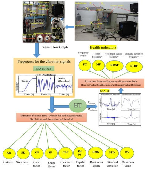
The proposed technique includes two key stages. (i) SSA is a strong strategy for non-fixed and nonlinear signal examination. It has been widely utilized for cyclic movement identification in the intricated dynamical framework and trend extraction from geophysical, analysis of death series, and climatic time series [39,40,41]. It empowers intricated signal to be decreased into various explainable parts containing a set of cyclic oscillations, noise, and a trend. Also, the fundamental of the disintegration is orthogonal and complete. The flow diagram of SSA strategy and HT for rotary encoder signal disintegration can be seen in Figure 1. The SSA technique fundamentally contains two phases: (a) disintegration and (b) restoration. In the disintegration stride, the Hankel matrix (trajectory matrix) is constructed from the single-dimensional encoder signal. Then SVD is implemented to the Hankel matrix for obtaining unit-rank essential matrices. Every one of these organic matrices is distinguished, via its singular value ${\lambda }_i$ and eigenvector $U_i$. In the rebuilding stride, matrices that can be translated as oscillations and a trend are assembled jointly as per their merit esteems (period of eigenvector and singular value). In order to recreate the identical items, a diametrical average of corresponding matrices is performed. The extracted oscillations and trend can be additionally used for status checking and movement exactness analysis. The process of this strategy will be described in the next, and more clarification concerning essential SSA can be found in [27].

The primary SSA method is based on the disintegration of an estimate of the trajectory matrix based on L-lagged vectors of the signal. SSA algorithm consists of the following strides:

Stride 1: Embedding: The signal of the encoder gathered from encoders for the feedback control system, it can be supposed as single-dimensional time series $\delta =(w_1,w_2,w_3,\cdots ,w_N)$ of length structure a sequence $\left\{{\delta }_{(t)}\right\}$ of K-Dimensional vectors from the time series $\left\{w_{(t)}:t=1,2,\cdots ,N\right\}$. K is the embedded dimension; N is the number of observations in the time series. In order to execute the embedding, the signal of an encoder is delineated into a sequence of L-lagged copies $(N>L>1)$ and shape the Hankel matrix $\delta =R^{L\times K}(L=1+N-K)$, as illustrated in Equation (1). For encoder signal disintegration, it is proposed to choose L as a minimum (N/2) to obtain the optimum fineness of approximate separation [17].

$$\delta =\left[\begin{array}{ccccc}{w}_1& w_2& w_3& \cdots & w_k\\ w_2& w_3& w_4& \cdots & w_{k+1}\\ w_3& w_4& w_5& \cdots & w_{k+2}\\ ⋮& ⋮& ⋮& \ddots & ⋮\\ w_L& w_{L+1}& w_{L+2}& \cdots & w_N\end{array}\right]$$

(1)

Stride 2: Singular value decomposition: In this stride, the quadrate matrix $Q=\delta {\delta }^T$ is adjusted to obtain the eigenvalues $({\lambda }_1,{\lambda }_2,{\lambda }_3,\cdots ,{\lambda }_L)$ in reducing the order of amplitude $({\lambda }_1\ge {\lambda }_2\ge \cdots \ge {\lambda }_L\ge 0)$ and the equivalent eigenvectors $(U_1,U_2,\cdots ,U_L)$. Then $V_i={\delta }^T{U}_i/\sqrt{{\lambda }_i}$ $(i=1,2,\cdots ,\alpha )$ are derived with $\alpha =rank\delta$ (Typically $\alpha =L$ for authentic encoder signals). In this route, the Singular value decomposition of the Hankel matrix $\delta$ can be acquired as Equation (2).

$$\delta ={\delta }_1+{\delta }_2+{\delta }_3+\cdots +{\delta }_{\alpha }$$

(2)

where ${\delta }_i=\sqrt{{\lambda }_i}{U}_i{V}_i^T$. The matrices ${\delta }_i$ have rank one; such matrices are sometimes called elementary matrices. The gathering $\left(\sqrt{{\lambda }_i,}{U}_i,V_i\right)$ will be called $i$ the eigen-triple (ET) enumerated in the reducing order of its singular value $\sqrt{{\lambda }_i}$.

Stride 3: Duration assessment: Fundamentally, elementary matrices are distinguished via their singular value $\sqrt{{\lambda }_i}$ and eigenvector $U_i$. Additionally, the amplitude data supplied via the value of singular $\sqrt{{\lambda }_i}$, the merit extraction of the eigenvector influences the following stride of eigen-triple gathering significantly. The duration of the eigenvector $U_i$ is suggested in the SSA method to decide the provenance of every eigen-triple. It is proposed to determine a duration via the autocorrelation function as Equation (3) of eigenvector displays in Figure 2. The duration is looked for in the lag domain to locate the highest value after zero position. If such a duration does not subsist for eigenvector, at that point, the eigenvector can be deemed as a portion of the trend, and it’s a duration determined to be zero.

$$y_{U_i(\tau )}={\displaystyle \int U_i(\tau )U_i(t+\tau )}dt$$

(3)

Stride 4: Eigen-triple (ET) gathering: In this research, eigen-triple is distinguished via the period value of its eigenvector $U_i$ and its singular value $\sqrt{{\lambda }_i}$. The eigen-triple gathering technique is to collect fundamental matrices of the Hankel matrix $\delta$ depend upon the two principle merit values. The value of the period drawn along the indicators $i$ symbolizing the cyclicity merit is called the spectrum of the period. The value of singular drawn along the indicators $i$ expressing to the amplitude merit is called the spectrum of singular. As per the two merit (singular value and period value), fundamental matrices can be assembled into $j$ separate subgroups $(X_1,X_2,\cdots ,X_J)$ explainable as a trend, groups of oscillations with the same period and noise. Set a subgroup $X=\{i_1,i_2,\cdots ,i_g\}$. The eventual matrix ${\delta }_X$ conformable to the set $X$ is known as ${\delta }_X={\delta }_{i1}+{\delta }_{i2}+\cdots +{\delta }_{ig}$ the eventual matrices are calculated for the sets $X=X_1,X_2,\cdots ,X_j$. Moreover, expansion Equation (2) leads to the decomposition as Equation (4).

$$\delta ={\delta }_{X_1}+{\delta }_{X_2}+\cdots +{\delta }_{X_j}$$

(4)

Stride 5: Diametrical Averaging: It is to convert every eventual matrix $\delta$ of the gathered disintegration Equation (3) back into a rebuilt string of longitude N. In this route, the authentic encoder string $\left\{{\delta }_1,{\delta }_2,\cdots ,{\delta }_N\right\}$ is split into an aggregate of j rebuilt substring as Equation (5):

$$w_n={\displaystyle \sum _{k=1}^j{\stackrel{⌣}{w}}_{n(n=1,2,3,\cdots ,N)}^{(k)}}$$

(5)

Every rebuilt substring can be translated as oscillations of the same period, noise and a trend as per the Eigentriple gathering technique. The reconstructed trend is neglected from entering the next step because it is a monotonic function. Immediately the procedure of SSA is completed, the spline normalizes applied to each reconstructed oscillation and reconstructed residual in order to ready to the second stage. HT is additionally broadly utilized in the signal demodulation. When the mechanical shortcomings happen, the gathered vibration signals are commonly modulated. Therefore, signal demodulation can isolate the carrier component and modulation component. Also, the flaw merits are usually hidden in the modulation component. It is necessary for us to apply the signal demodulation using HT. The HT is implemented on both reconstructed oscillation and reconstructed residual to extract the IA, and IF of the analyzed signal and describes the signal more regionally.

In generic, $\stackrel{⌢}{R}(t)$ represents the reconstructed oscillations or reconstructed residual from SSA method of an arbitrary signal $r(t)$ then HT for the reconstructed oscillations or reconstructed residual is described as:

$$\stackrel{⌢}{R}(t)=H[R(t)]=\frac{1}{\pi }{\displaystyle \underset{-\infty }{\overset{\infty }{\int }}\frac{R(t)}{t-\tau }}d\tau =R(t)\ast \frac{1}{\pi t}$$

(6)

where the symbol ‘∗’ denotes convolution operation. According to the HT, the analytic signal can be expressed as:

$$r(t)=R(t)+j\stackrel{⌢}{R}(t)=a(t)\exp \left[j\phi (t)\right]$$

(7)

where $j=\sqrt{-1}$

$$a(t)=\sqrt{R^2+{\stackrel{⌢}{R}}^2}\mathrm{and}\phi (t)=arctan(\frac{\stackrel{⌢}{R}}{R})$$

(8)

Here, $a(t)$ is the IA and $\phi$ is an instantaneous phase. The IF is defined as $\omega =\frac{d\phi }{dt}$. Then the Hilbert envelope spectrum can be calculated as:

$$h(f)={\displaystyle \underset{-\infty }{\overset{\infty }{\int }}\sqrt{R^2(t)+{\stackrel{⌢}{R}}^2(t)}}\exp (-j2\pi ft)dt$$

(9)

In this way, the SSAHT on a non-stationary and non-linear signal extracts its IF and IA. Which is beneficial to determine source oscillations and residual to evaluate the health conditions and fault detection for the industrial robot.

3. Numerical Simulation

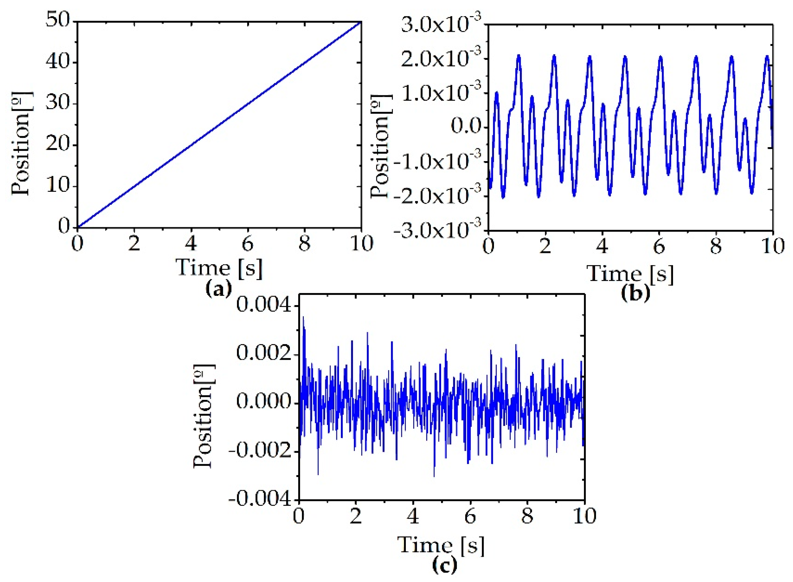
The Signal of the rotary encoder is complex, even the machine is running at a steady speed. Also, a linearly rising trend, feeble oscillations with minor amplitudes are subsisted in the position signal because of mechanical flaws. Moreover, the oscillations can be nonlinear because of the non-fixed running state. Besides, measurement of noise is also unavoidably comprised in the signal. In this work, the upper factors, the whole has been taken into the matter of illustrating the achievement of the suggested technique. Deem arm robot having two degrees of freedom, is feed at a steady speed of 5°/s with payload fell at a descending stance illustrates in Figure 3, where we took the signal of the rotary encoder near from the end effector. In another word, one degree of freedom in this simulation, just joint 2 for the signal of encoder comprises three components: (a) A linear trend $y_{trend}$, (b) oscillations with the same period $y_{oscillations}$, and (c) noise $y_{noise}$ as depicted in Equation (10). The encoded signal 10 s is obtained, and its sampled at 50 Hz. The trend is 4 orders of amplitude higher than the noise. The oscillations contain trio harmonics $(y_{o1},y_{o2},y_{o3})$ of 0.8 Hz with variable initial stages. Their magnitudes are exponentially adjusted to emulate the non-fixed operating circumstance. White noise with equal power as the oscillations is added. Figure 4 illustrates cyclic oscillations, noise, and the authentic waveform of the trend.

In order to experience, the SSA technique, the Hankel matrix (L = minimum(N/2)) is primarily structured, and SVD is implemented to the matrix. Singular values $\sqrt{{\lambda }_i}$ log given in Figure 5a to set the magnitude of the conformable ET. Moreover, periods of eigenvectors $U_i$ are shown in Figure 5b to locate the oscillations together the identical duration. The values of period and values of singular of the initial twelve eigen-triples (ETs) are specified in

Table 1. The period and singular value of eigentriples (number 1–12).

ET number	1	2	3	4	5	6
Singular value	181,550.7	948.8	7.9 × 10−5	7.3 × 10−5	5.4 × 10−5	5.24 × 10−5
Period (s)	0	0	1.792	1.792	1.322	1.322
ET number	7	8	9	10	11	12
Singular value	3.1 × 10−5	2.99 × 10−5	5.14 × 10−6	5.12 × 10−6	5.09 × 10−6	4.81 × 10−6
Period (s)	1.491	1.491	0.778	0.778	0.778	0.301

.

From Figure 5a,b and Table 1, it can be seen that the initial two eigen-triples ET2 and ET1 have the highest magnitudes and as well are not cyclic. The initial two ETs are collected jointly to rebuild the trend.ET3 and ET4 have the next highest magnitude with an identical period 1.792 s. So, ET4 and ET3 represent the highest cyclic components of the signal. Also, ET6 (ET5) and ET8 (ET7) the identical period for their period are 1.322 s and 1.491 s. Harmonics are ever persistently subsisted in the authentic mechanical signal. The fourth ET4 to ninth ET9 harmonics are missing. Thus, the rest of eigen-triple is not treated as a portion of the cyclic oscillations. Just ET3 to ET8 are collected together to reconstruct the oscillations.

$$\begin{array}{l}{y}_{trend}=5t\\ y_{oscillations}=y_{o1}+y_{o2}+y_{o3}\\ y_{o1}={10}^{-3}\times \exp (t/35)\times \cos (2\times \pi \times 0.8\times t+1.2)\\ y_{o2}={10}^{-3}\times \exp (-t/35)\times \cos (2\times \pi \times 1.6\times t+3.1)\\ y_{o3}={10}^{-3}\times \exp (-t/22)\times \cos (2\times \pi \times 2.4\times t+2.2)\\ y_{noise}={10}^{-3}\times randn(t)\end{array}$$

(10)

The reconstructed oscillations and trend are specified in Figure 6a–c demonstrates the errors between the (theoretical) ideal solution and reconstructed components through subtraction. The root means square (RMS) of errors are 0.000137664° and 0.000256858° for the rebuilt trend and oscillations respectively, which is lower than (0.1) of the magnitude of the oscillations in the existence of similar to white noise. It can be inferred that the SSA strategy accomplishes an agreeable decomposition outcome with minimal signal deformation both in phase and amplitude. EMD strategy is also executed here for comparison. EMD technique is not able to decompose the authentic signal. Due to that, the trend is many orders of amplitude higher than the oscillations. The situation without the presence of the trend is inspected here, and signal for the EMD technique to the procedure is clarified as $y=y_{oscillations}+y_{noise}$. The acquired IMF is plotted in Figure 7.

In order to rebuild the cyclic oscillations, numerous arrangements of IMFs have been attempted to perform a lower error. The reconstructed oscillations of the EMD method are adopted, the IMF’s combine starts from IMF4 to last IMF because the first IMF element represents the feature of noise with high frequency. The second and third IMF describes the primary merits of partial discharge signals [5,42]. Thus, the IMFs collection, of $\{y_4(t),y_5(t),\dots ,y_8(t)\}$ can obtain an ideal outcome with a minimal root mean square of error 0.001275508°, and the rebuilt oscillations are appeared in Figure 8a.

A performance index (PI) is a common standard to measure the performance of the system and to determine the health condition through the features of the time domain. The signal of time domain collected from the rotary encoder to give changes when damage occurs in the harmonic reducer or gear. Both its distribution and amplitude may be different from those of the time domain signal of a standard harmonic reducer. Ten types of performance indices are utilized to examine the health condition of the system. Mean value ($\overline{R}$) reflects the average of a signal. Root amplitude (RA), the maximum value (MV), and Root mean square (RMS) reflects the vibration amplitude and energy in the time domain. Standard deviation (STD), skewness (SK), kurtosis (KR), clearance factor (CLF), crest factor (CF) and shape factor (SF) may be used to represent the time series distribution of the signal in the time domain. The specific formulations of these features are given in

Table A1. Time domain features extraction.

Name	Formula	Name	Formula
Mean value ($\overline{R}$)	$\overline{R}=\frac{{\displaystyle {\sum }_{j=1}^m{R}_j}}{m}$	Kurtosis (KR)	$KR=\frac{m{\displaystyle {\sum }_{j=1}^m\left(R_j-\overline{R}\right)}}{{\left({\displaystyle {\sum }_{j=1}^m{\left(R_j-\overline{R}\right)}^2}\right)}^2}$
Standard deviation (STD)	$STD=\sqrt{\frac{1}{\left(m-1\right)}{\displaystyle \sum _{j=1}^m{\left(R_j-\overline{R}\right)}^2}}$	Skewness (SK)	$SK=\frac{{\displaystyle \sum _{j=1}^m{\left(R_j-\overline{R}\right)}^3}}{\left(m-1\right){\left(STD\right)}^3}$
Maximum value (MV)	$MV=\max \left|R_j\right|$	Crest factor (CF)	$CF=\frac{\max \left|R_j\right|}{\sqrt{\frac{1}{m}{\displaystyle {\sum }_{j=1}^m{\left(R_j\right)}^2}}}$
Root amplitude (RA)	$RA={\left(\frac{{\displaystyle {\sum }_{j=1}^m\sqrt{\left|R_j\right|}}}{m}\right)}^2$	Root Mean Square (RMS)	$RMS=\sqrt{\frac{1}{m}{\displaystyle {\sum }_{j=1}^m{\left(R_j\right)}^2}}$
Shape factor (SF)	$SF=\frac{\sqrt{\frac{1}{m}{\displaystyle {\sum }_{j=1}^m{\left(R_j\right)}^2}}}{\frac{1}{m}{\displaystyle {\sum }_{j=1}^m\sqrt{\left|R_j\right|}}}$	Clearance factor (CLF)	$CLF=\frac{\max \left|R_j\right|}{{\left(\frac{{\displaystyle {\sum }_{j=1}^m\sqrt{\left|R_j\right|}}}{m}\right)}^2}$

.

Table 2. Features time domain of the error indexes of reconstructed oscillations via the empirical mode decomposition (EMD) technique and the singular spectrum analysis (SSA) technique and the error indexes of the rebuilt residue via SSA technique. (Unit: °).

Features	EMD (Oscillations)	SSA (Oscillations)	SSA (Residual)
RMSE	0.001275508	0.000256858	0.000233266
Kurtosis	0.086044	0.573306	−0.013496031
Skewness	0.13488739	0.20492204	0.290127491
Crest factor	3.368909	3.546686	2.664382861
Maximum Value	0.004297	0.0009109	0.000621509
Standard deviation	0.001274813	0.000257115	0.000231719
Clearance factor	5.002846263	5.391546032	4.190179051
Shape factor	1.257620556	1.275556037	1.285310062
Root amplitude	0.000858925	0.000168967	0.000148325
Mean Value	7.08321 × 10−5	−2.0038 × 10−7	−2.87435 × 10−5

compares with features time domain of the error indexes containing features are good indicators for incipient faults, KR, SK, CF, SF, CLF, STD, RA, RMSE, $\overline{R}$ and the MV of the error between the SSA technique and the EMD technique. The rebuilding error via the EMD technique is no less than 5 times bigger than rebuilding error through SSA technique. As well as we can extract features for reconstructed residual by the SSA method are given in Table 2, while the EMD technique cannot be reconstructed. It can be inferred that the SSA technique outflanks the EMD technique in three aspects. The first aspect, oscillations separated via the SSA strategy, are improved than the EMD technique in terms of exactness. The second aspect, the SSA strategy, can disintegrate the signal of the rotary encoder in the existence of a high trend, while the EMD technique cannot. The third aspect, residual includes useful information by SSA method, but in EMD method the remaining is too small to continue, or it becomes a monotonic function from which no more IMF can be extracted, also hardly contains any useful information reflecting mechanical flaws.

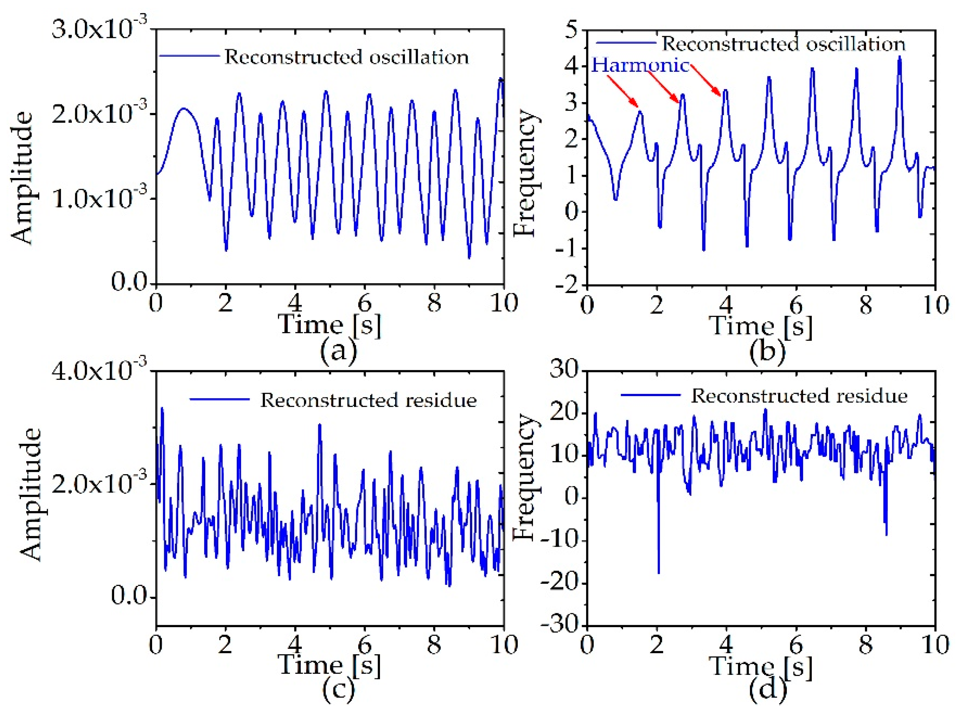
The reconstructed trend, reconstructed oscillation, and reconstructed residual are calculated by the SSA method. The reconstructed trend is neglected because it is a monotonic function. Therefore, we have implemented the HT for reconstructed oscillations and reconstructed residual. The simulated response signals are illustrated in Figure 9.

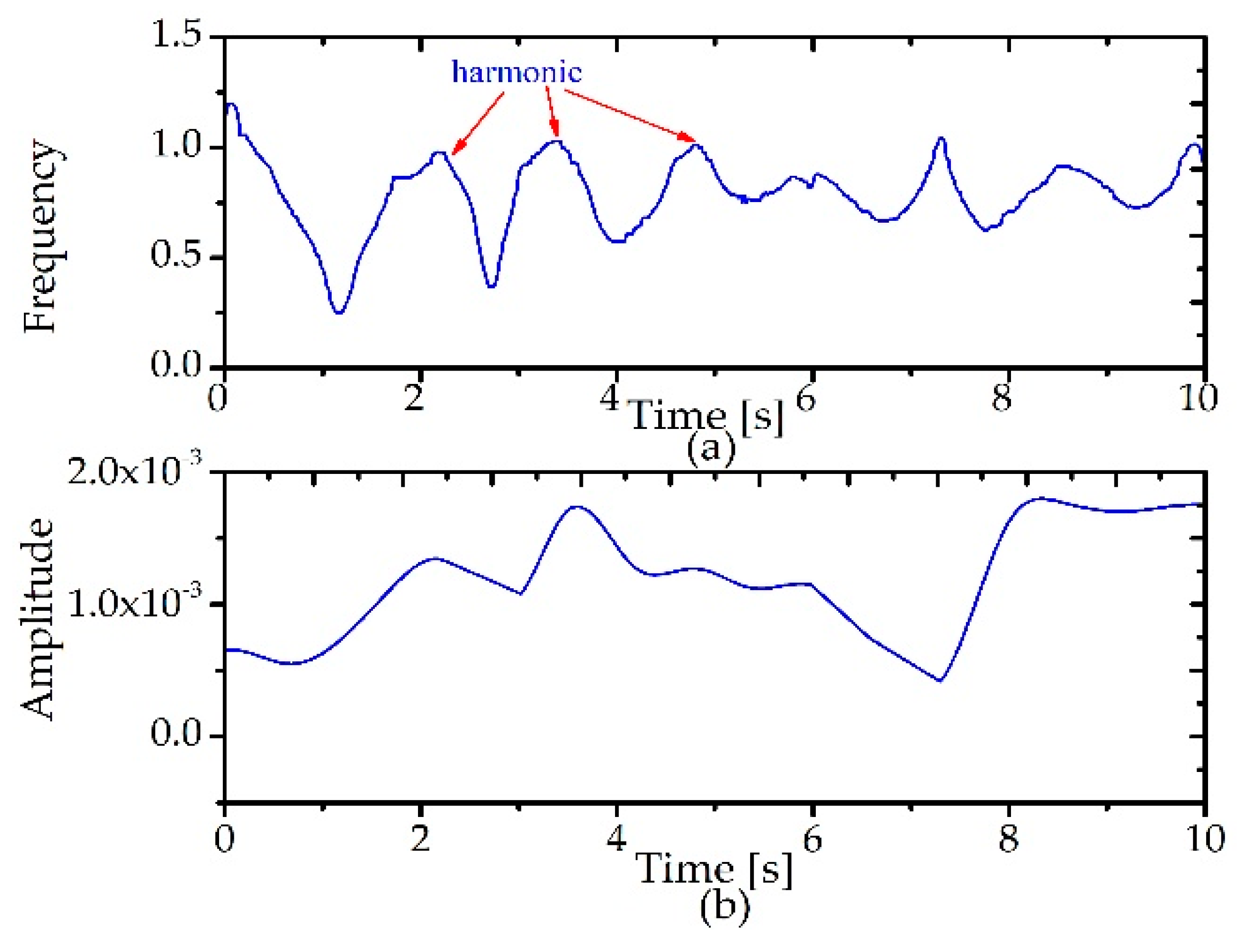
It can be seen that IA, and IF is extracted by HT for reconstructed oscillations and reconstructed residual after applied SSA algorithm for the rotary encoder signals. It can be observed in Figure 9a the IA have harmonics and skew-symmetric. So, IF have harmonics and also skew-symmetric illustrated in Figure 9b. The IA and IF for reconstructed residual is given in Figure 9c,d, respectively. The IF and the IA for reconstructed oscillations by the EMD method appears in Figure 10a,b.

In this paper, four types the features of the frequency domain parameters are extracted from the frequency spectrum of a gear vibration signal. These features of the frequency domain parameters may include information that is not existing in the features of the time domain parameters. Mean frequency (MF), indicates the vibration energy in the frequency domain. Frequency Center (FC) and Root mean square frequency (RMSF) show the position changes of the main frequencies. Standard Deviation Frequency (STDF) describes the convergence degree of the spectrum power. Therefore, these frequency domain features can reflect the mechanical health conditions from different aspects. The specific formulations of these features are given in

Table A2. Frequency domain features extraction.

Name	Formula	Name	Formula
Mean frequency (MF)	$MF=\frac{1}{v}{\displaystyle \sum _{v=1}^v{R}_v}$	Root mean square frequency (RMSF)	$RMSF=\sqrt{\frac{{\displaystyle {\sum }_{v=1}^v{f}_v^2{R}_v}}{{\displaystyle {\sum }_{v=1}^v{R}_v}}}$
Frequency center (FC)	$FC=\frac{{\displaystyle {\sum }_{v=1}^v{f}_v{R}_v}}{{\displaystyle {\sum }_{v=1}^v{R}_v}}$	Standard deviation frequency (STDF)	$STDF=\sqrt{\frac{{\displaystyle {\sum }_{v=1}^v{\left(f_v-FC\right)}^2{R}_v}}{{\displaystyle {\sum }_{v=1}^v{R}_v}}}$

.

Table 3. Features frequency domain for the error indexes of rebuilt oscillations via the empirical mode decomposition Hilbert transform (EMDHT) technique and the singular spectrum analysis and Hilbert transform (SSAHT) technique. (Unit: °).

Features	EMDHT (Oscillations)	SSAHT (Oscillations)	SSAHT (Residual)
RMSF	8.91860581	1.72450458	2.040854602
MF	0.00167641	0.000305109	0.000268524
STDF	16.29435848	0.841860912	0.922030442
FC	7.656280457	1.50505357	1.820699692

compares with frequency domain features of the error indexes for reconstructed oscillations containing, RMSF, MF, STDF, and FC of the error between the SSAHT technique and the EMDHT technique. The reconstruction error RMSF by EMDHT technique is at least 5 times greater. It can be inferred that the SSAHT technique outperforms the EMDHT technique on two sides. Firstly, reconstructed oscillations extracted via SSAHT technique are better than EMDHT technique in terms of accuracy. Secondly, the reconstructed residual obtained from SSAHT method is better than the EMDHT method in terms of physically meaningful because the residual in EMDHT method it is either a monotonic function or a constant. Besides Table 3 depicts, features frequency domain for reconstructed residue by SSAHT.

4. Validation of the Experiment

Fluctuations or oscillations of a servo motor axis during operating can lead to a fault in industrial robots. Even though, with full control of closed loop, warranty for its authentic predictability and no dynamical error is not ensured. In order to distinguish the source and evaluate the magnitudes of the oscillations is of fundamental significance for the condition monitoring of industrial robots. It will also be beneficial for accuracy improvement and active flaw pursuit. Figure 11 demonstrates a signal flow graph for the comprehensive perspective of our experiment instruments. The robot arm control system primarily contains a servo drive module, a servo control module, and a mechanical arm body.

The EtherCAT protocol is used between the control module and the servo drive module for high data transmission speed and fast response time. The servo drive module drives the servo motor to drive the six degrees of freedom manipulator for various motions. The EtherCAT coupler (EK1100, Beckhoff, Germany) is mainly used to connect two EtherCAT-capable hardware. The connected hardware can be EtherCAT terminal module, controller, and driver. Moreover, the primary purpose is to translate the transmission signal information from Ethernet 100 BASE-TX into E-bus signal. The company’s control cabinet-style industrial PC, the model is C6925, the controller is equipped with an Intel^® Celeron^® M ULV processor (Intel, Santa Clara, CA, USA), and the TwinCAT3 operating version of the automation software can be an excellent way to achieve multi-axis motion control and data processing. In this work, two degrees of freedom is required to accomplish the task, and each degree of freedom requires a motor and a driver. In order to save the installation size of the experimental platform and to meet the control requirements of the manipulator, a drive-driven TAMAGAWA motor (Ts4609, TAMAGAWA SEIKI CO., LTD., Iida, Japan) with two drives was selected, with the leader drive company’s harmonic reducer to achieve the mechanical arm joint drive. The cooldrive RC6 drive is a multi-axis driver that enables two motors to be driven by the single drive, which is compact and saves installation space. The driver supports EtherCAT communication protocol, enabling subtle levels of communication with the controller. Its drive starter debugging software can adjust not only the motor’s current loop, speed loop, encoder, and other related parameters but also real-time monitoring of motor operation. The servo motor for multi-pass TS series is AC servo motor. The servo motor, combined with the 17-bit absolute encoder of the TAMAGAWA, not only accurately records the position of motor motion but also does not lose the position because of re-power.

The TAMAGAWA absolute encoders (Ts4609, TAMAGAWA SEIKI CO., LTD., Iida, Japan) used in the system are equipped with a lead mercury battery for preserving the motor position and initializing the acquisition. The harmonic reducer has become an important transmission component in the modern industry because of its light weight, small volume, high transmission ratio, and relatively high efficiency. The reducer used by the picker is a harmonic reducer produced by the leader drive company. Compared with the general planetary reducer, the harmonic reducer has a large deceleration ratio. After the Industrial Computer (IPC) receives the motion signal transmitted by the host PC, after judging and recognizing the motion control task, the path curve for the falling of the end effector payload when the test is carried out, this experiment took two degrees of freedom, joint 1 move toward X-axis, and then joint 2 progress toward Y-axis. The velocity control experiment was achieved for the industrial robot, implemented two cases of velocity 6°/s and 12°/s with payload (4 kg). The target position is transferred to the servo drive system by Numerical Control (NC) task to drive the manipulator motion. In the meantime, the rotary encoder of the servo motor will feedback the position information of the manipulator movement and reach the target position.

The TWINCAT3 software can scan and identify the servo drive model and the basic parameter information of the servo motor through the EtherCAT communication protocol. The axis variables in the PLC can then be connected to the virtual axes in the NC to correlate to the actual servo motor. That allows the movement of the motor to be controlled by changing the variables in the control program. The NC axis in the TWINCAT3 software also requires parameter settings. The important parameter is the scaling factor, i.e., the angle or distance at which the controller rotates the joint at each position of the pulse manipulator. For the experimental platform, the servo motor is equipped with a 17-bit absolute value encoder of the TAMAGAWA and its binary output code. In other words, the motor shaft has (2¹⁷ = 131,072) a pulse output of 1 cycle (360°) per revolution. The manipulator is a rotating joint, but the reduction ratio of the harmonic reducer is different, and the scaling factor parameters corresponding to the joint end are not the same. Take the joint axis 1 as an example; the reduction ratio is 1:100, then the arm joint end per revolution (360°) corresponding pulse number is (2¹⁷ × 100), so the joint corresponding is scaling factor = 360°/(2¹⁷ × 100) = 0.00002746582031. Similarly, the parameters of other joint motors can be set according to the size of the deceleration ratio.

In this research work, the X-axis, the signals of the rotary encoder of a three-axis robot arm to joint 1 and the Y-axis rotary encoder signals of 3-axis robot arm to joint 2, were examined via the suggested technique to determine magnitudes of both Y-axis and X-axis feed oscillations and their central source. Figure 12 shows the path Coordinate of Y-axis in joint 2 and X-axis in joint 1. We analysis the Y-axis and X-axis of the rotary encoder signal for two joints. The real departure range is not taller than 50° at each joint to guarantee that the scope for experiences of analysis. The servo motor (TS4609) drives the harmonic reducer to rotate during coupling, and harmonic reducer decodes rotational movement to move the robot arm.

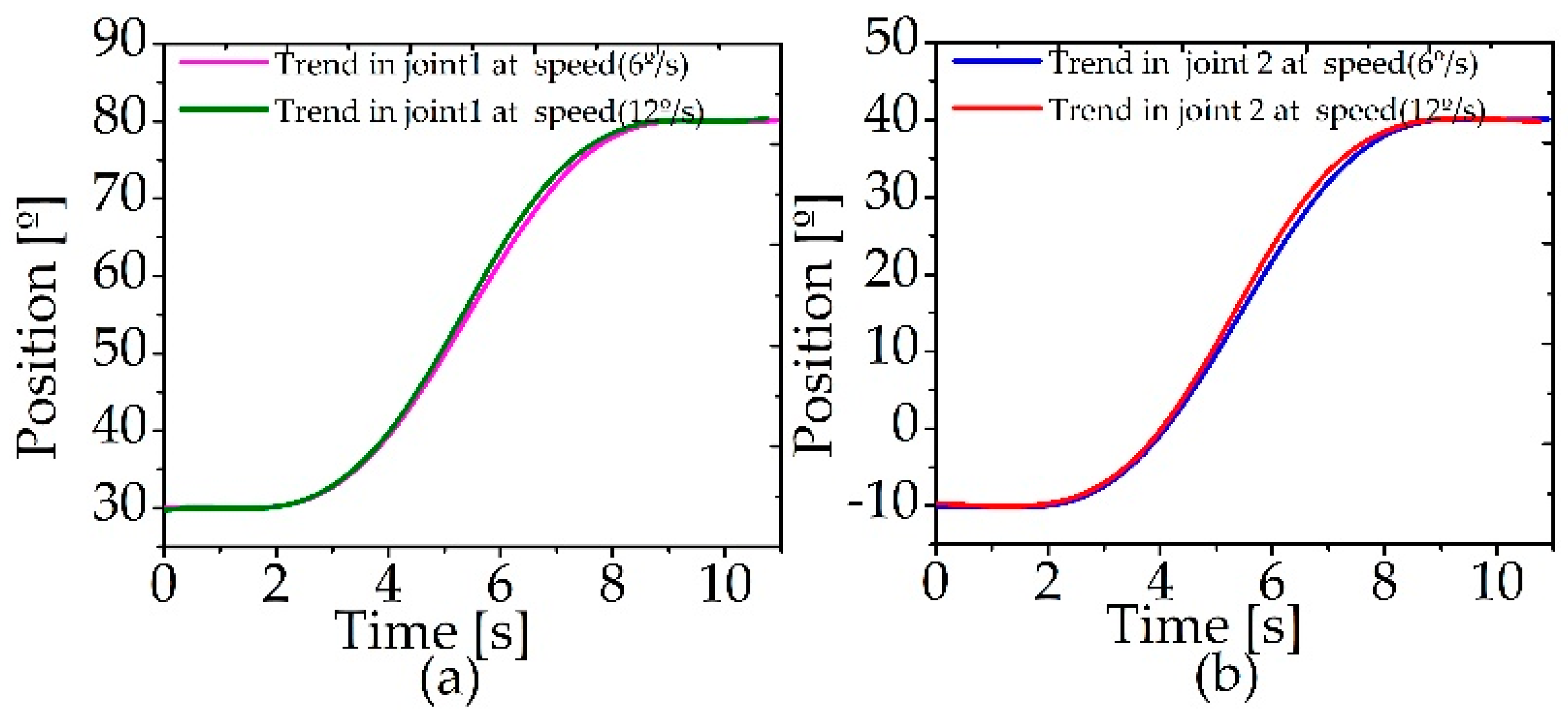
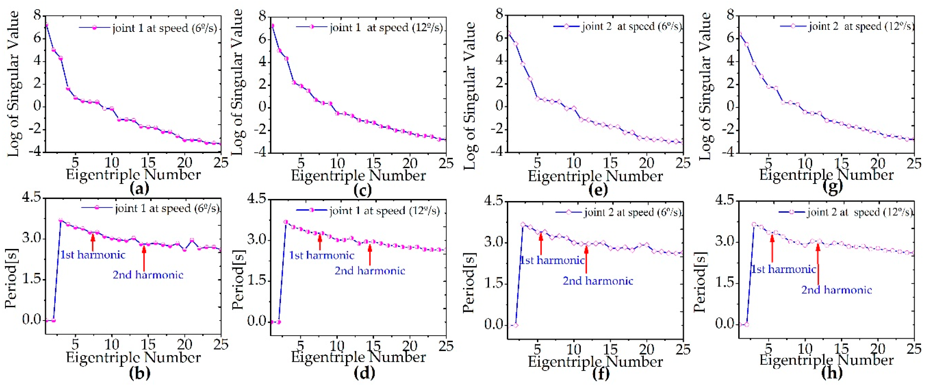
A rotary encoder fabricated via TAMAGAWA is mounted in joint 1 to measure the X-axis position and Joint 2 to measure the Y-axis position. The sampling frequency is 500 Hz. Figure 13 displays the position data of the encoder signal measured in every case. Also, it depicts the real departure range in each joint equal to 50°. In order to apply the SSA method, the Hankel matrix is mainly constructed and used SVD. Period spectrum and singular spectrum are shown in Figure 14 to recognize the period and magnitude of the same eigentriple to position for every case.

The values of period and values of singular of the first twenty eigen-triples are specified, in

Table 4. The period and singular value of eigentriples for the position of the encoder signal (number 1–20).

ET Number	Joint 1 in Speed (6°/s)		Joint 1 in Speed (12°/s)		Joint 2 in Speed (6°/s)		Joint 2 in Speed (12°/s)
	Singular Value	Period (s)	Singular Value	Period (s)	Singular Value	Period (s)	Singular Value	Period (s)
1	1.8 × 1007	0	1.8 × 1007	0	2,635,163	0	2,644,657	0
2	107,318	0	111,655	0	317,203	0	317,464	0
3	19,790.7	3.6902	21,217.2	3.67715	5322.3	3.66745	6635.28	3.65321
4	43.1552	3.53148	167.026	3.49206	272.198	3.57287	510.02	3.55023
5	6.33478	3.42325	78.3248	3.41162	5.07148	3.39794	66.4329	3.35218
6	3.35876	3.38021	30.9813	3.32284	4.19045	3.39794	47.3334	3.35218
7	2.69656	3.24304	4.94857	3.26623	2.85211	3.20412	2.70376	3.20412
8	2.60678	3.24304	2.53093	3.26623	2.69356	3.25527	2.53302	3.02602
9	0.71372	3.09342	2.39923	3.14983	0.72777	3.17918	1.74194	2.99109
10	0.69943	3.02112	0.30923	3.00732	0.72193	3.00918	0.38023	2.88677
11	0.07666	2.96548	0.30241	3.02119	0.0722	2.96614	0.30112	3.04119
12	0.07647	2.93848	0.19953	3.07918	0.07159	2.96614	0.29353	3.04119
13	0.06419	3.03141	0.0811	2.88138	0.03649	2.97772	0.0714	2.88081
14	0.01881	2.81291	0.06126	2.94939	0.02756	3.01072	0.06152	2.97081
15	0.01674	2.81291	0.04936	2.94939	0.01835	2.81291	0.03854	2.94448
16	0.01482	2.8451	0.02189	2.88791	0.01803	2.80291	0.02302	2.84291
17	0.00656	2.78736	0.01869	2.81291	0.00574	2.84336	0.01805	2.83291
18	0.00633	2.74036	0.01049	2.81341	0.00558	2.74036	0.0132	2.86332
19	0.00279	2.83251	0.00878	2.75786	0.00191	2.91925	0.00874	2.74936
20	0.00125	2.60206	0.00603	2.74036	0.00158	2.92742	0.00683	2.78456

. Figure 14 depicts every state and Table 4; it can be concluded that the first two eigentriples are equivalent to the trend, since ET1 and ET2 have the highest magnitudes, and their period values are zero in all cases. Table 4 shows that the highest position oscillation of the rotary encoder signal has the period of both joint 1 and joint 2 at 6°/s are 3.6902 s and 3.66745 s, respectively. The periods represent 22.141°, 22.0044°, which is the nearly half the period of the rotation of joint. Then the period of both joint 1 and joint 2 at 12°/s is 3.67715 s and 3.6532 s, respectively. The period represents 44.125° and 43.83°, which is the nearly total period of the rotation of the joint.ET3 and ET4 have the next highest magnitude in all cases. Thus, the ET3 and ET4 represent the highest periodic components of the signal in all cases.ET5 and ET6 first harmonic in joint 2 of both 6°/s and 12°/s have the same period 3.39794 s and 3.35218 s respectively. While ET7 and ET8 first harmonic in joint 1 of both 6°/s and 12°/s have the same period 3.24304 s and 3.26623 s. Also, ET11 and ET12 second harmonic in joint 2 of both 6°/s and 12°/s have the same period 2.96614 s and 3.04119 s respectively. Thus, the ET14 and ET15 second harmonic in joint 1 of both 6°/s and 12°/s have the same period 2.81219 s and 2.94939 s. Since the 3rd harmonic is not discovered, other eigentriples are gathered jointly as the residual. Harmonics are ever persistently subsisted in real mechanical signals.

Figure 15 depicts the position of the encoder signal disintegration outcomes as the residual, oscillations, and the trend in every state. Harmonic reducer synchronizes with detected oscillations, which implies that the primary oscillations of the feed movement originate from the harmonic reducer. It can be seen that the cyclic oscillations are magnitude adjusted in order to inspect the relevance between the position oscillations and feed velocity. Additionally, Figure 15c,f,j,m depicts extract residual from the original signal. It can be seen that the noise signal of the payload movement and its fall during the robot arm motion in our experiment.

The outcomes at two velocities with the 4 kg payload are likewise specified for joint 1, and joint 2 comparisons are presented in Figure 16. The label of X-axis is transformed from time to position for a preferable offering. The generic forms of the position variations display uniformity both in phase and magnitude, and the specifics of the waveforms display that the magnitude of the first harmonic raises with increasing velocity. The SSA technique safely detaches the main oscillations, tend, and the remainder (other less essential noise and oscillations) at various speed. As aforesaid, transforming position signal to acceleration or velocity signal via differential likewise detects the feeble changes and can be beneficial for condition monitoring. Velocity oscillations by a rotary encoder in joint 1 and joint 2 are given in Figure 16. RMSE computations of both velocity oscillations case and position oscillations case for each case are illustrated in

Table 5. The RMSE of both velocity oscillations and position oscillations at two speeds in joint 1 (X-axis) and joint 2 (Y-axis), (unit: °).

Number of the Case	Name of the Case	RMS of Position Oscillations	RMS of Velocity Oscillations
1	Joint 1 in speed (6°/s)	0.04901807	0.09673056
2	Joint 1 in speed (12°/s)	0.10675341	0.15303526
3	Joint 2 in speed (6°/s)	0.04975681	0.096346142
4	Joint 2 in speed (12°/s)	0.12972809	0.153124265

for joint 2 and joint 1. Figure 16, Table 5 and

Table 6. The RMSE of both velocity residual and position residual at two speeds in joint 1 (X-axis) and joint 2 (Y-axis), (unit: °).

Number of the Case	Name of the Case	RMS of Position Residual	RMS of Velocity Residual
1	Joint 1 in speed (6°/s)	0.01126470	0.041149651
2	Joint 1 in speed (12°/s)	0.01169334	0.044110695
3	Joint 2 in speed (6°/s)	0.003082208	0.062490225
4	Joint 2 in speed (12°/s)	0.009783509	0.066625612

demonstrate that velocity for both oscillations and residual are changed significantly at two speeds. If oscillations and remaining of the robot arm’s motion are translated through velocity, the computed oscillations and residual are capable of working velocity and afford vicarious outcome concerning motion precision. By disparity, position oscillations extracted via the SSA technique provide a harmonious result at different working velocity and are valuable for movement precision investigation.

The IA and IF with time for both the position and velocity for each from oscillations and residual in joint 1 and joint 2 are acquired during the payload movement and its fall during robot arm motion. The IA and IF are extracted by a Hilbert transform after applied SSA algorithm for the rotary encoder signals in four cases is specified in Figure 17 and Figure 18. It can be observed that the first two columns in both Figure 17 and Figure 18, all IA and IF in both position oscillations and velocity oscillations are either skew-symmetric or symmetric. Additionally, IA and IF in both position residual and velocity residual in both Figure 17 and Figure 18. It can be seen that the noise signal of the payload movement and its fall during robot arm motion very clear. The general shapes of the position oscillations display flexibility both in the IA and IF at two joint, and brief facts of the waveforms define that IF of the first harmonic increases with increasing speed to double. The IA and IF in both position and velocity for each oscillation and residual in each case for the rotary encoder signals. It can be seen that the cyclic oscillations are amplitude adjusted. To examine the connection between the oscillations and increase velocity. The outcomes at two velocities are also given for comparison in Figure 17 and Figure 18, and

Table 7. Mean Frequency (MF) and Standard Deviation Frequency (STDF) for both position and velocity for the reconstructed oscillations by the SSAHT technique. (Unit: °).

Number of the Case	Name of the Case	Position		Velocity
		MF	STDF	MF	STDF
1	Joint 1 in speed (6°/s)	0.065939527	0.067225709	0.131400448	0.070655828
2	Joint 1 in speed (12°/s)	0.126189095	0.077888917	0.180450162	0.073309907
3	Joint 2 in speed (6°/s)	0.068035684	0.062512932	0.122092424	0.077472362
4	Joint 2 in speed (12°/s)	0.129950486	0.117940516	0.180776083	0.078673834

. The MF and STDF are calculated of both position oscillations, and velocity oscillations are given in Table 7.

Table 8. Mean Frequency (MF) and Standard Deviation frequency (STDF) for both position and velocity for the reconstructed residual by the SSAHT technique. (Unit: °).

Number of the Case	Name of the Case	Position		Velocity
		MF	STDF	MF	STDF
1	Joint 1 in speed (6°/s)	0.006773656	1.086009685	0.040069533	11.33145285
2	Joint 1 in speed (12°/s)	0.009464425	1.031458131	0.040088014	25.59869192
3	Joint 2 in speed (6°/s)	0.00258905	4.457890508	0.047326328	12.88027215
4	Joint 2 in speed (12°/s)	0.008046206	1.249922629	0.049415548	13.52058735

shows the MF and STDF are calculations for both position residual and velocity residual in each case for the rotary encoder signals. The signal residual contains valuable features of the data extracted by the proposed method in each joint at an industrial robot such as MF and STDF are calculated for both position residual, and velocity residual. The MF indicates the vibration energy in the frequency domain, and the STDF is displayed the position change of MF, which are dominant in the frequency spectrum. These features reflect the mechanical health conditions volatility and dispersion of the data are given in Table 8.

The proposed method safely separates primary oscillations and the residual at two speeds and give reliable result at different working velocity. As well as detecting weak position oscillations and velocity oscillations in the time domain and frequency domain. As aforementioned, it also reveals the weak oscillations and can be helpful for condition monitoring and motion accuracy analysis.

5. Conclusions

In this study, the rotary encoder signal, after appropriate processing, can also be efficiently utilized for the health observation of energy performance of industrial robots-system. Combined Singular spectrum analysis and Hilbert transform (SSAHT) are proposed to detect weak position for both (oscillations & noise) extraction. Firstly, the proposed SSA technique decomposes the rotary encoder signal into noise, oscillations, and a trend with signals deformation both in phase and magnitude. The cyclicity merit of eigenvector computed via autocorrelation is suggested for eigentriple (ET) gathering in the singular spectrum analysis technique. There is a clear physical meaning for that feature for concerning periodic machine movement, which makes choice eigentriple simple. Secondly, the proposed HT to extract the IA, the IF for both oscillations and noise as per the outcomes of simulation, the SSAHT strategy outflanks the EMDHT technique regarding precision and capability. The following conclusions are drawn from the outcomes obtained:

• The oscillations extracted through the SSA technique have a higher precision compared with the EMD technique;
• The SSA technique can decay an encoder signal when a large trend is present, whereas the EMD technique cannot;
• Residual includes advantageous information, obtained by SSA method but in EMD method the residual is too small to continue, or it becomes a monotonic function from which no more IMF can be extracted, also hardly contains any useful data reflecting mechanical flaws;
• The IA and IF are extracted by the SSAHT technique have features better than EMDHT technique of reconstructed oscillations;
• The SSAHT technique extracts the IA and IF of residual, has beneficial information to evaluate the health conditions while the EMDHT technique cannot;
• The IA and IF in both position and velocity for each oscillation and residual in four cases are obtained from through the payload movement, and its fall during robot arm movement to determine source oscillations and the residual are valuable data to assess the health status and fault detection for energy performance of the industrial robot.