1. Introduction
An oscillating water column (OWC) is a well-known type of wave energy converter (WEC). The incident waves cause the water level inside the OWC chamber to oscillate. The oscillations of the water column cause a pressure differential between the atmosphere and the settling chamber. This pressure differential drives a turbine, mounted on top of the chamber, and mechanical power is produced. This mechanical power is then converted to electricity by a directly coupled electric generator.
In the current WEC industry, initiatives are required to reduce the cost of harnessing renewable energy and drive down the levelized cost of energy (LCOE) [
1]. Efficient wave to wire performance of the OWC converter requires design optimisation of different parts of the conversion chain [
2]. Research on the OWC, Power Take-Off (PTO), and generator units has been expanded in recent years to identify efficient designs of these elements and maximize the energy conversion of the whole system [
3].
To date, self-rectifying turbines have been almost extensively used in OWC plants, due to the capability to operating in bidirectional flows which eliminated the requirement for air valves.
The Wells and impulse turbines are the two extensively studied types of self-rectifying turbines, and the test results of their aerodynamic performance are most available compared to other OWC turbines. Extensive reviews and detailed analyses of Wells and impulse turbines can be found in [
4,
5,
6,
7,
8,
9,
10]. Research on self-rectifying Wells and impulse turbines was performed considering their full-scale size and their performance under real operational conditions [
3]. The analysis was based on a stochastic approach, and the pressure oscillations of the OWC were assumed to be random Gaussian. Falcao et al. conducted research on the optimization of air turbines for operation in a bottom-standing OWC [
11], in which a Wells and a bi-radial impulse turbine were evaluated regarding their speed in energetic sea states. The bi-radial turbine is a highly efficient alternative to the self-rectifying axial flow turbines, which has a symmetrical geometry with respect to a plane perpendicular to its axis of rotation [
5,
12,
13].
Different versions of unidirectional turbines have been studied in the twin-turbine concepts [
12,
14,
15,
16,
17]. A twin-turbine topology employs two unidirectional turbines instead of a bi-directional turbine. Each turbine is active during a single direction of flow in the system (direct mode) and is considered idle during the reverse direction (reverse mode). The numerical and experimental studies of the twin-turbine configurations have mainly been performed on axial flow unidirectional turbines. Design modifications of this twin-turbine configuration have obtained a peak efficiency of around 70% in the direct mode [
15,
17,
18,
19]. However, the global efficiency of the twin-turbine also requires the efficient operation of the turbine in reverse mode [
20]. Pereiras et al. [
16] were the first to consider negative torque produced in the reverse turbine in the efficiency calculations of the twin-axial turbines. Research on the application of unidirectional radial impulse turbines in twin-turbine OWC configurations is still in progress. Rodriguez et al. [
21] improved the geometry of a unidirectional radial turbine in twin-turbine topology for higher resistance to flow in the reverse mode, however, the turbine’s direct peak efficiency was significantly low (approximately 40%). They later focused on optimising this turbine’s design for efficiency maximization in the active mode, while keeping the strong flow blockage in the reverse mode [
22].
A vented OWC is an alternative concept for rectifying airflow through the air turbine. The OWC column is fitted with an array of one-way air valves so that as the water column rises the air escapes from the chamber, bypassing the turbine with very little backpressure. Consequently, the water column rises further compared to that in a conventional OWC. The incoming wave energy is temporarily stored in water column heave which is added to outflow energy transferred to the air turbine when the water column falls, allowing capture of energy over the full-wave energy cycle with a unidirectional air turbine [
23]. The power output of different air turbine and OWC configurations under irregular sea waves was evaluated by Ansarifard et al. [
24]. Two unidirectional radial turbines, intended to be used in a vented OWC, were compared by a conventional turbine-OWC system regarding their full-scale size, rotational speed, and power conversion under real sea conditions using the experimental data of irregular wave in vented and bidirectional OWCs.
Employing optimisation tools in the numerical studies can provide a refined approach for identifying different aspects of the turbine design. Employing response prediction algorithms can aid investigation of a larger design space and allow a more reliable solution. Understanding the impact of design variables on the objective functions can ensure a fast and reliable exploration of the optimum turbine designs. Several studies have focused on optimising the turbine designs for OWC and identifying the most sensitive parameters affecting the turbine performance [
3,
22,
25]. Impact of the rotor blade profile was studied on performance of the Wells turbines [
26,
27,
28], and optimisation methods were used to explore an optimum blade design by varying the camber line and blade thickness. A 2D blade profile of an impulse turbine was optimised in [
29], a 3D blade geometry was created by stacking the 2D profile spanwise and a 5% efficiency improvement was obtained. Mohamed et al. [
30] employed systematic optimisation to investigate the blade shape of a reaction turbine using the same parameters as is used in an airfoil design. The genetic algorithm and computational fluid dynamics (CFD) techniques were used to optimise the rotor blade shape of an axial turbine for efficiency maximization and improvement of the power output over a wide range of flowrates. The optimised airfoil obtained an 11.3% increase of the power output compared to the initial design of the blade. Design optimisation methods were also used by Mohamed and Shaaban [
31] to predict the performance of a Wells turbine with self-pitch controlled blades. They used parameters in a non-symmetric airfoil shape to identify the optimum design. Optimised sweep angle of the rotor blade of a wells turbine was studied using the surrogate modelling [
32]. The optimum blade was reported to have a backward sweep angle at the mid-section and a forward angle at the tip and improved the torque by 28%. Apart from the blade profile, the number of blades and guide vanes were also investigated using the optimisation methods. A multi-fidelity analysis coupled with the CFD was performed to maximize the efficiency of impulse turbine used with an OWC [
33].
The authors of this work have completed several studies on design improvement of a unidirectional radial turbine. An analysis of the losses at different sections of a radial inflow turbine was performed, and significant energy losses were reported due to the radial-axial transition of flow at the elbow section. To overcome this problem, the authors suggested an increase of the casing height from the inlet to the outlet of the turbine and elbow sections, which achieved 10% total efficiency improvement [
24]. In addition, the downstream section was design optimised for proper coupling with the inflow radial turbine, and it was concluded that a diffuser-shaped duct with a diffusion angle of seven degrees leads to a significant recovery of the kinetic energy [
34].
This study focuses on the design optimisation of a unidirectional radial turbine for maximum efficiency in the outward flow direction. The investigation was conducted using CFD, and design optimisation techniques were used to maximise the efficiency of the rotor and upstream guide vanes in a radially-outward-flow configuration over a range of steady-state flowrates. A list of design variables was considered in the creation of the parametric CAD geometry of the rotor blades and the upstream guide vanes. The impact of design variables on the turbine efficiency, output power, input power and flow resistance were analysed, and the most sensitive parameters were identified.
In this article, the parametric geometry and input parameters are defined in
Section 2. The numerical setup and validation of the numerical model are outlined in
Section 3 and
Section 4, respectively. In
Section 5, the setup of the optimisation study and the output parameters are explained, followed by the discussion of the results. In
Section 6, the significance of the optimisation study is discussed by comparing the performance of the initial and optimum outflow turbines. In addition, the outflow turbine has been evaluated regarding the rotor energy exchange in a centrifugal radial configuration. Finally, in conclusion, the main findings of this work are provided.
2. Turbine Geometries
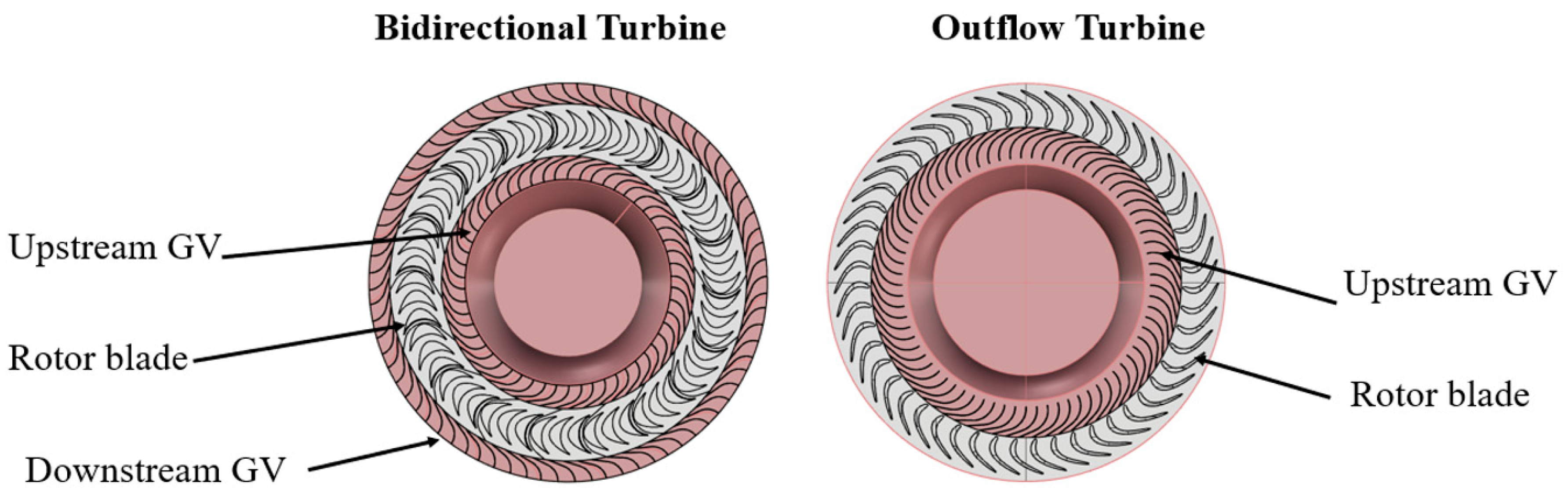
A bidirectional configuration of a radial turbine extracted from a study by Setoguchi et al. [
35] was used for validation of the numerical method and creation of a reference for an initial centrifugal (outflow) radial turbine. The bidirectional turbine geometry has main characteristics presented in
Table 1. The initial outflow turbine geometry was designed according to the main geometrical characteristics of the bidirectional turbine. The geometries of the duct and upstream guide vanes (UGVs) were chosen to be similar to that of the bidirectional turbine. In addition, the inner diameter, number of upstream guide vanes and the rotor blades (RBs) were equal in both turbines (more details can be found in [
35]). The main differences were, first, using asymmetric rotor blades appropriate for an outward flow direction. Secondly, removing the downstream guide vanes (DGVs) since only outward flow direction was considered as operational. Schematics of the bidirectional geometry and the initial outflow turbine are shown in
Figure 1.
A parametric 3D model of the initial turbine geometry was generated using the CAESES software [
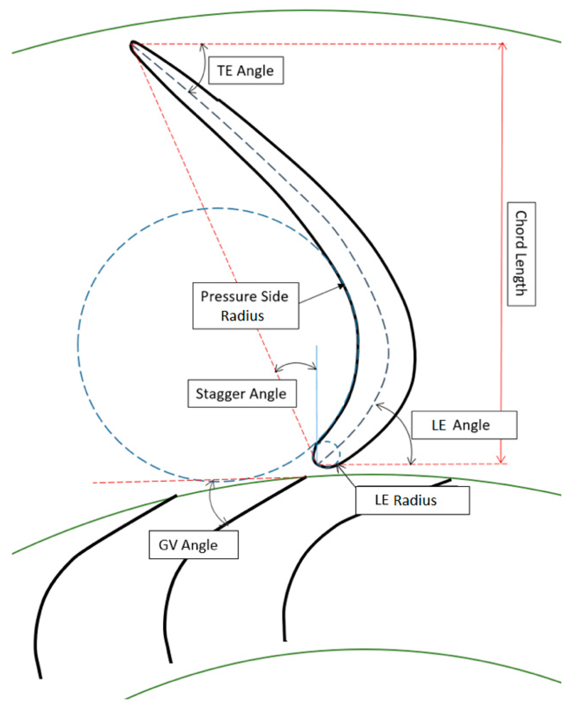
36]. Selection of the base geometry for the rotor blade needed to be done regarding some specific characteristics of the turbine. To ensure acceptable conversion of the input power, an asymmetric blade profile with highly flexible curves in the suction and pressure sides was needed. Therefore, a base blade profile with 11 design variables was created using the software database [
36]. This parametric blade shape could offer enough flexibility to create a large design space by varying a large set of parameters. However, the computational cost and simulation time were directly associated with the number of input parameters. Therefore, to reduce the computational cost, the optimisation study was focused on the shape of the rotor blades and their adjustment with the guide vanes. Among the parameters available to control the blade’s 2D profile, six parameters were chosen [
37,
38]. These parameters were the leading-edge radius (LE Radius), chord length, pressure side radius (PS Radius), leading-edge angle (LE angle), stagger angle and trailing edge angle (TE angle).
Figure 2 illustrates these parameters in the parametric blade profile. In addition to the blade profile, the setting angle of the upstream guide vanes (GV Angle) was included in the input parameters list.
Table 2 determines the lower and upper bounds of the input parameters and their values in the reference design (the initial outflow turbine geometry).
3. Numerical Modelling
Numerical simulation tools were employed to optimise the design of the initial outflow turbine in steady-state. The computational simulations were conducted using ANSYS CFX. The turbine performance was described by a set of parameters [
35]: torque coefficient
, input power coefficient
, turbine efficiency
and flow coefficient
as given by
The detailed definitions of the variables contributing to these coefficients are given in the nomenclature section. The quasi-steady assumption of the flow was assumed because the rotating frequency is much higher than the frequency of the wave cycle in the OWC chamber [
21,
39]. As an external modelling software was used for the creation of the parametric geometry, the turbo-mode tool in ANSYS-CFX was used to set up the problem to ease the iterative process of the optimisation study. The Moving Reference Frame (MRF) approach was used to set up the steady model by assuming that the rotor rotates at a constant speed of 120 rad/s and considering a frozen rotor interface between the rotor and the stationary domains. In this approach, both stationary and rotating domains are solved at steady-state with a frame change model to connect them. It is clear that the actual condition is unsteady, and an unsteady analysis delivers more accuracy, however, it could lead to increased solution time. Thus, the MRF model was chosen to provide an acceptable computational overhead for the large number of design simulations required in an optimisation study. However, to evaluate the errors due to ignoring the unsteady interaction between the rotating and the stationary domains, the optimum design of the optimisation study was later analysed in a transient model (as will be described in
Section 6.3).
The simulations were performed at a Reynolds number of
. The flow was assumed incompressible and the realizable k-ε turbulence model was selected due to being economical in terms of computational time. This turbulence model has been utilized in many similar studies in the field and accurate results were obtained [
40,
41]. Other turbulence models such as k-ω and the hybrid SST could obtain more accurate results in this study as a strong effect of the wall, adverse pressure gradients, and flow separation phenomena are present in the simulations. However, these turbulence models were more computationally expensive than the k-ε turbulence model and were not economical considering the simulation time of the optimization study. This choice of turbulence model can reduce the accuracy of results at higher flowrates, however, according to the typical operation of turbines in an OWC, the peak efficiency falls in smaller flow coefficients, and the results of this analysis are still reliable.
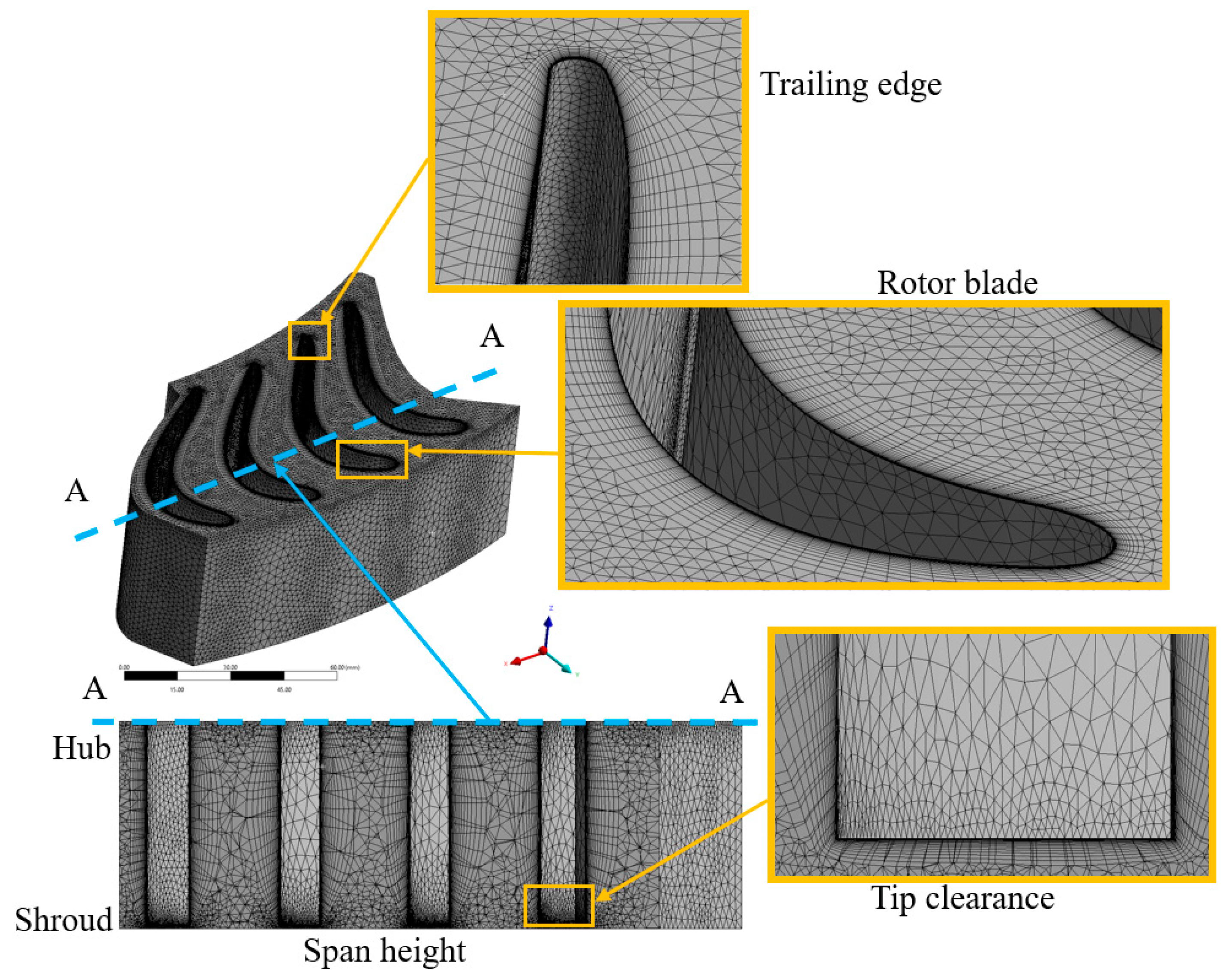
Periodic boundaries were set on the sides of each domain, and the interfaces between the rotating and stationary domains were set to the frozen rotor. A pitch angle ratio close to 1 was set at the interface, by applying the passage and alignments of 2/52 at the downstream, 2/51 at the upstream and 3/73 at the rotor section. The computational domain contained three parts: duct, rotor upstream domain and the rotor domain. To reduce the computational overhead, an angular section of the geometry including three upstream guide vanes and two rotor blades were used instead of the whole geometry as shown in
Figure 3. The boundary conditions of uniform total pressure at the inlet and uniform static pressure at the outlet were considered. Total pressure values from 0.5 kPa to 20 kPa were set at the inlet to provide a range of non-dimensional flow coefficients from
= 0.25 to
= 2.5. The convergence criteria were set to an RMS residual target of
.
The ANSYS meshing program was used to create the mesh for numerical simulations. The size function was set on proximity and curvature to provide greater control over the mesh. Inflation layers were used in the meshing to allow the solver to determine the forces on walls, flow incidence, secondary flows and separation [
42]. Separation affects the drag and pressure drop and its accurate prediction relies on resolving the velocity gradients normal to the wall. In the viscous sublayer of a turbulent boundary layer, these velocity gradients are very steep and use of inflation layers permits the accurate capture of the near-wall flow behaviour and resolves the viscous sublayer directly (low y
+ ~1) [
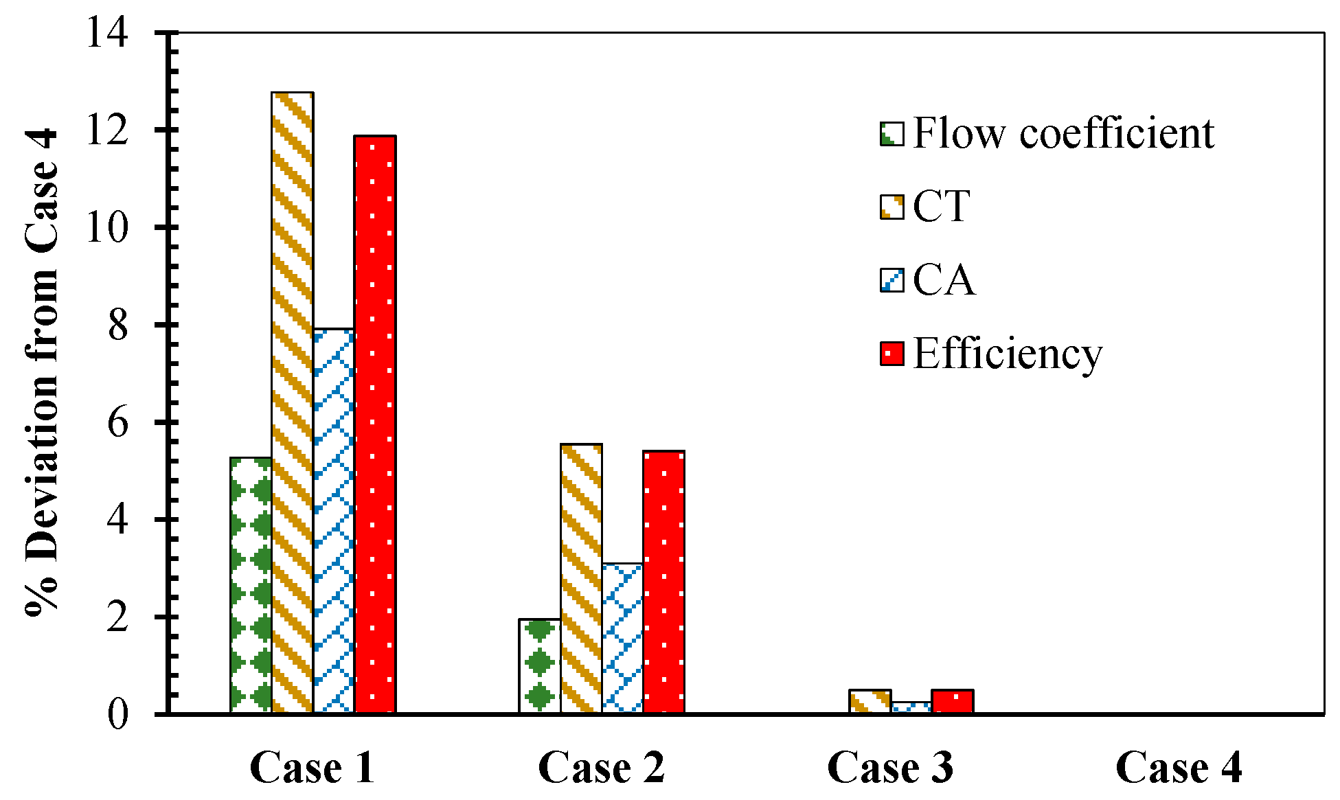
43]. In this study, twenty inflation layers were applied with the transition ratio of 0.5 and a growth rate of 1.2. The minimum size and proximity settings were varied to study mesh independence by creating four cases with 0.25, 0.5, 1 and 2.5 million tetrahedral cells in the main volume mesh.
Figure 4 illustrates the percentages of deviation from case 4 with the maximum number of cells (2.5 million), where case 1 denotes the minimum number of cells (0.25 million). It is obvious that case 1 obtained the least accurate results in comparison to other cases with over 12% deviation in
. Case 2 provides a maximum deviation of about 6% and the discrepancy of results in case 3 is practically nil. Therefore, case 3 with a total number of 1 million cells was used for the CFD simulations to save time and CPU usage. A schematic of the mesh used in the simulations is shown in
Figure 5. It should be noted that the mesh setting was kept constant while the cell number varied by changes applied to the initial geometry in the optimisation study.
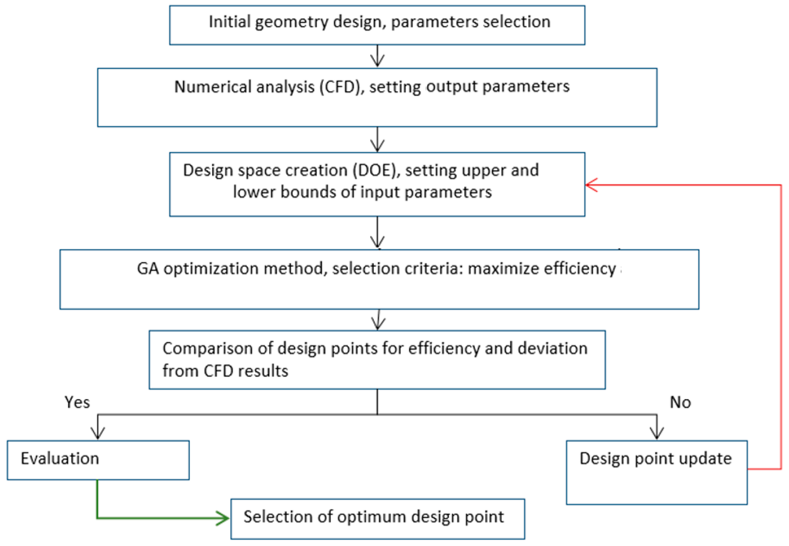
5. Numerical Optimisation of the Outward Flow Radial Turbine
The optimisation study is an iterative process which begins by performing CFD simulations on the initial geometry of the inflow turbine. Then, the output parameters are defined, and design exploration is used to create a design population by varying the input parameters. In this study, design of experiments method (DOE) was used to determine the design space and characterize the turbine performance based on a minimum number of actual analysis runs. The DOE conducts a series of experiments within the specified variation range of the input parameters set and minimizes the quantity of the required analysis runs to determine the parameters impacts. The central composite design (CCD), based on a fractional factorial design was used to reduce the number of experiments by sacrificing less meaningful high-order interactions [
44]. A second-order analysis was used with the capability to model the interaction between the input parameters and surface curvatures appropriately. The general form of a second-order model explained in [
45] is:
where,
and
are the design variables,
the tuning parameter and
the number of parameters. In the CCD, an optimal design space is considered with two criteria: the degree of non-orthogonality of regression terms (or variation inflation factor (VIF)), and the position of sample points (Leverages or the diagonal elements of the design matrix) [
46]. Using this method, the design space contains a centre point,
design points located at the −α and +α position on each axis of the selected input parameters and
factorial points located at −1 and +1 positions along the diagonals of the input parameters space. Where α is selected such that both the maximum VIF and the maximum leverage are the minimum possible and
is the fraction of the factorial design and is a function of
. As an example, CCD for two design variables consists of four factorial points, four axial points, and one central point as schematically shown in
Figure 7. In this study, seven input parameters were considered and
fractional factorial designs used, which halved the number of experiments from the
factorial designs.
The response surface function is used in the next step to fit the actual analysis data characterized by the DOE and sample a surrogate model. The response surface optimisation is used to perform an indirect optimisation analysis and evaluate the optimum candidate design predicted by various methods [
47]. It provides a smooth and continuous mathematical formulation by interpolating between discrete design points of the DOE. The response surface optimisation method allows the design points to be predetermined by the DOE and permits simultaneous solving of the response-surface design points and multiple optimisations. In the current study, the Genetic Aggregation (GA) response surface algorithm was used to predict the optimum design point. GA is a meta model that selects the most appropriate response surface for each output parameter based on the genetic algorithm. It solves different response surfaces in parallel, analyses them regarding their accuracy and the stability in the cross-validation and can be a single response surface or a combination of several different response surfaces [
46]. In the optimisation step, the genetic algorithm was used as the optimiser which is a well-known approach in turbomachinery design optimisation) [
44,
45,
47]. In the genetic algorithm, feasible solutions are specified according to the bounds of the optimisation problem and the optimal solution is explored by analysing the maximum allowable Pareto front [
48]. In this study, maximization of the total to static efficiency (defined in Equation (3)) was specified as the optimisation objective. In addition, other turbine characteristics such as torque coefficient (Equation (1)), input power coefficients (Equation (2)) and flow coefficient (Equation (4)) were set as the secondary output parameters.
Figure 8 shows the iterative process of the optimisation study.
6. Results and Discussions
The optimised outflow turbine geometry of this study is shown in
Figure 9 with the design characteristics indicated in
Table 3.
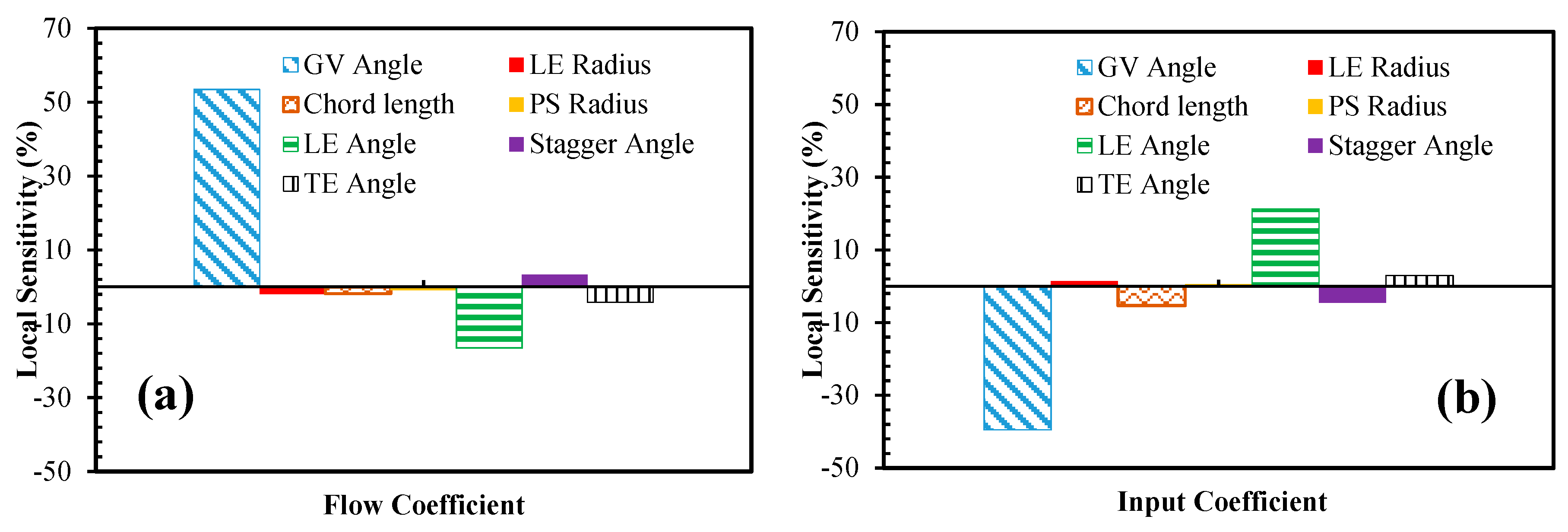
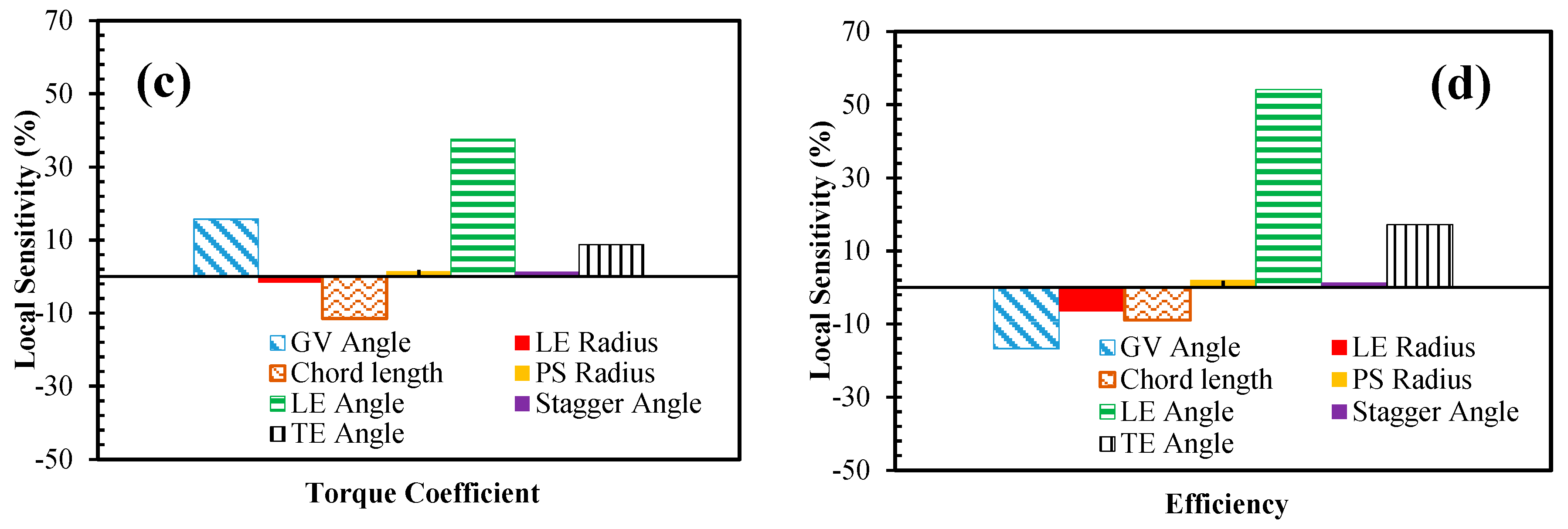
The sensitivity of output parameters regarding the rate of changes applied to each input parameter was evaluated and shown in
Figure 10. The local sensitivity statistics were generated regarding the trend of the efficiency at the optimum design point and determined the rate of impact of each parameter on the efficiency variations. The local sensitivity is an exploration tool included in the response surface, which analyses the weight of each input parameter on the output parameters independently [
43]. If the increase of a parameter fulfils the objective function in the optimisation journey, that parameter is shown with a positive sign. In other words, the positive and negative bars in
Figure 10 show the increase and decrease of the parameter, respectively, with respect to its initial values in the reference geometry.
Considering the local sensitivity data illustrated in
Figure 10a, the angle of the guide vane (GV angle) affects the flow coefficient significantly. It is obvious that an increase of the GV angle leads to a wider area between the upstream guide vanes and reduces the flow incidence and losses at the rotor upstream to a high extent. The LE angle has a reverse effect, which can be explained by the role of this parameter in shaping the flow passage between the rotor blades. Increasing the LE angle in the rotor geometry of this study leads to a narrower blade to blade area and increases the resistance to the flow at the rotor inlet. The input coefficient is mainly sensitive to GV angle and the LE angle as shown in
Figure 10b. It is obvious that a higher GV angle causes a lower input coefficient. As the input parameter is related to the pressure, this can be justified regarding the influence of the GV angle on the pressure drop and losses in the turbine domain. This fact was also reported in a study by Setoguchi et al. [
35], in which for a fixed LE angle, there is a reverse relationship between the angle of the upstream guide vanes and the
CA parameter. The LE angle affects the input coefficient by shaping the blade flow passage and affecting the
VR term in the definition of
CA in Equation (2). As illustrated in
Figure 10c, the LE angle has the highest contribution among the variations in torque coefficient. Increasing the LE angle causes more inclination of the rotor blade and reduces the area and flow velocity at the mean radius of the rotor (known as
AR and
VR respectively). These terms contribute to the
CT as defined in Equation (1). The sensitivity of the turbine total to static efficiency to the studied input parameters is shown in
Figure 10d. It is observed that the efficiency is mostly affected by the LE angle followed by the GV angle and TE angle. The LE angle being an effective parameter on both
CT and
CA, has a positive effect on the efficiency due to its higher impact on the torque coefficient than the input coefficient. The negative effect of the GV angle can also be explained by its effect on the input power and flow coefficient terms.
It should be noted that changes to the combination of input parameters lead to the optimum design point, however, the 3D response of efficiency based on the two most sensitive parameters (LE angle and GV angle) is illustrated in
Figure 11. This figure shows that the optimum efficiency was identified clearly within the specified variation bounds of these two parameters.
6.1. Comparison of the Initial and the Optimum Outflow Turbine Geometries
After finding the optimum design for the outflow turbine, its operation was compared to the initial outflow geometry determined in
Table 2. A comparison of the flow rate versus total pressure drop of the initial and the optimised geometries is illustrated in
Figure 12a. It is clearly shown that for a given range of the total pressure drop, the optimised geometry acts more resistive to the flow rate than the initial geometry. Considering the local sensitivity figure of the flow coefficient shown in
Figure 10a, the flow rate is mainly affected by the GV angle and the setting angle. According to the geometrical characteristics of the initial and the optimised designs (as mentioned in
Table 2 and
Table 3 respectively), both geometries have a close GV angle. Thus, the higher resistance of the optimised geometry can mainly be due to its 10 degrees higher LE angle compared to the initial geometry. For the same reason, the input coefficient of the optimised design (
Figure 12b) is significantly higher than that of the initial design, which can be due to the decreased flow velocity at the mean radius (
) of the optimised design. The term
, as shown in the Equation (2), has a reverse impact on the input coefficient values considering (
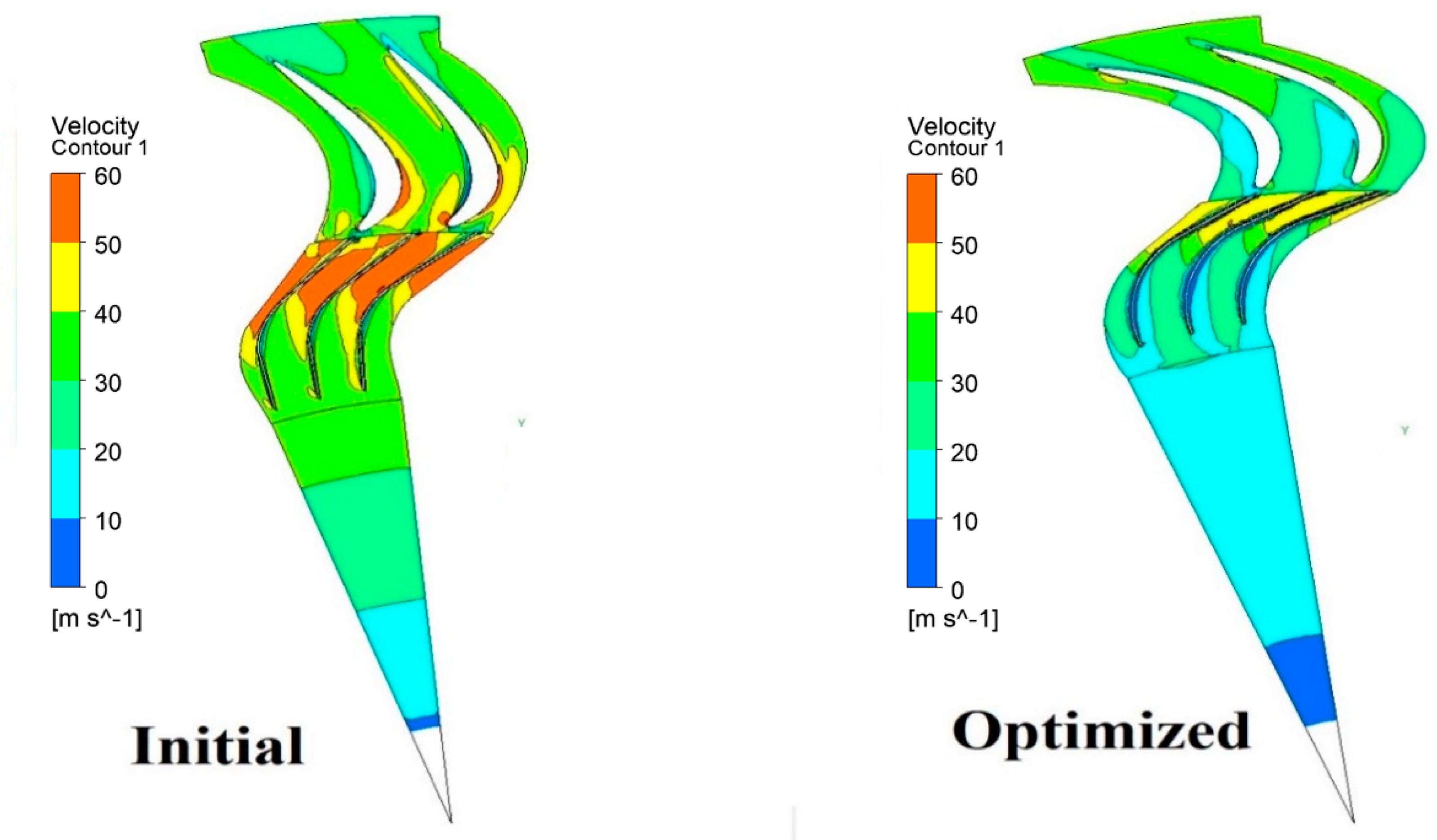
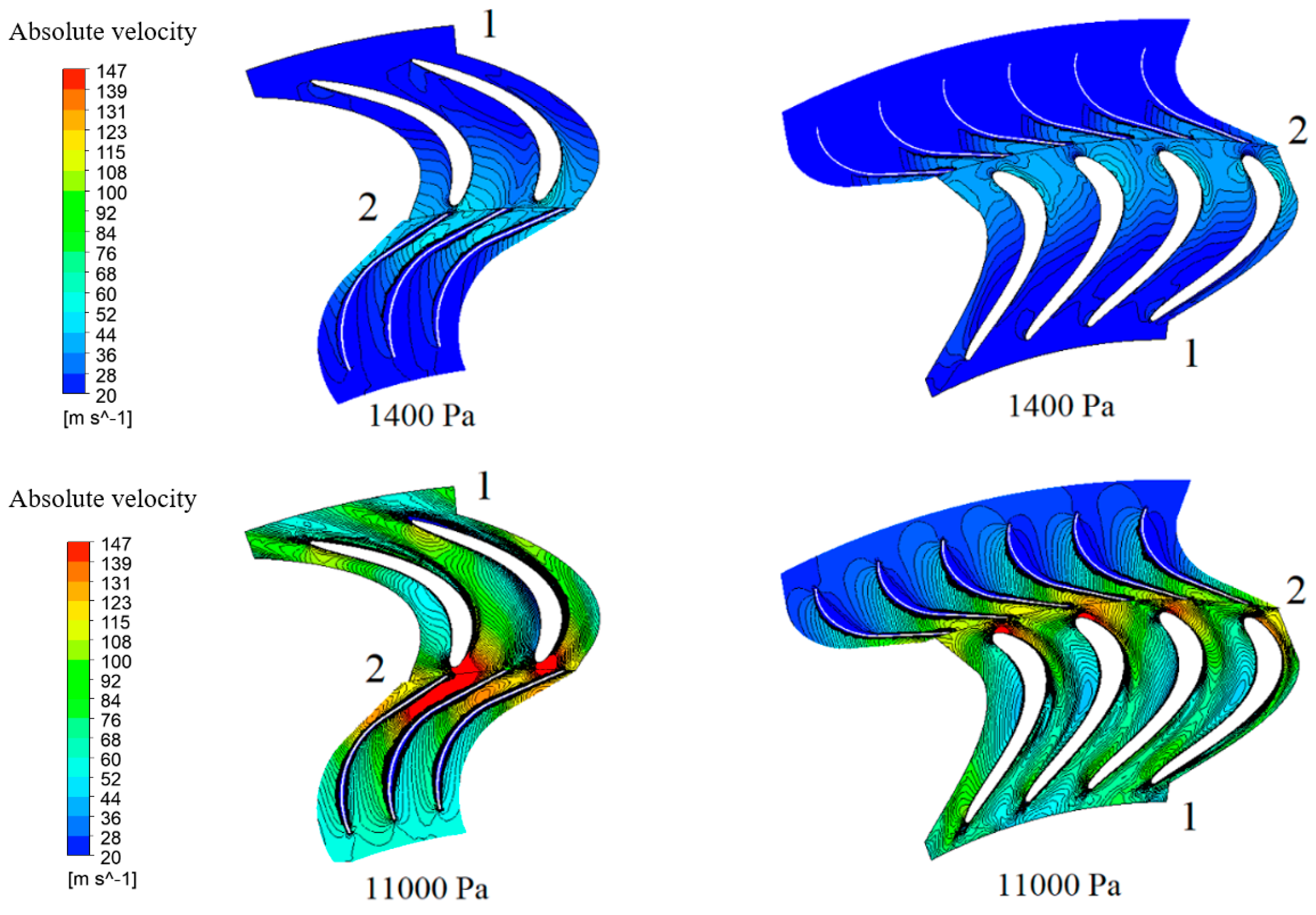
). Comparison of the velocity contours in the rotor domain of both geometries
= 1400 Pa, in
Figure 13, clearly illustrates the lower air velocity at the mid-chord of the optimised design.
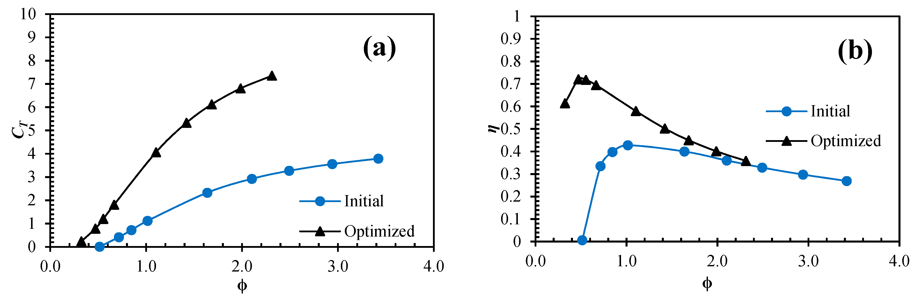
As illustrated in
Figure 14a, torque coefficient of the optimised design has improved significantly compared to the initial design, which according to the design characteristics of both geometries, is mostly due to 10 degrees higher LE angle and smaller chord length of the optimised design compared to the initial geometry. According to
Figure 14b, the optimised geometry has 30% higher peak efficiency than the initial design, which has been obtained by finding the optimum combination of the input parameters used in this study. For the optimised design, the operational flow range is smaller than the initial design and the peak efficiency point has moved towards smaller flow coefficients. This fact was previously explained by comparing the flowrate versus pressure drop of both geometries in
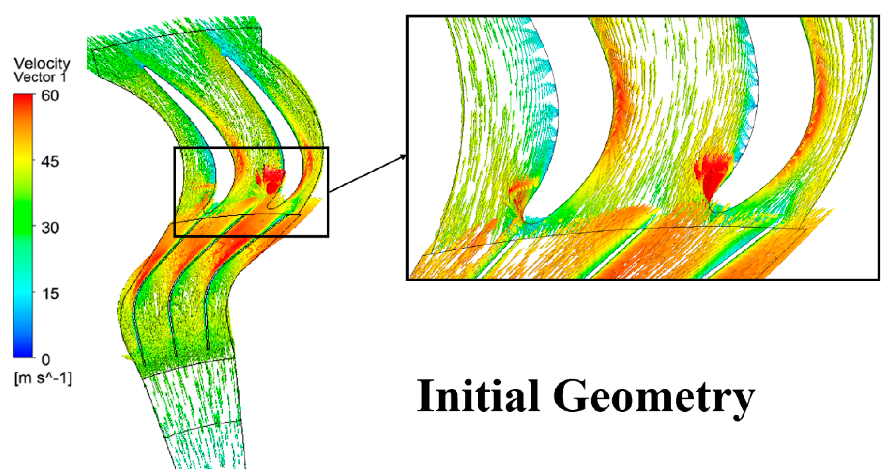
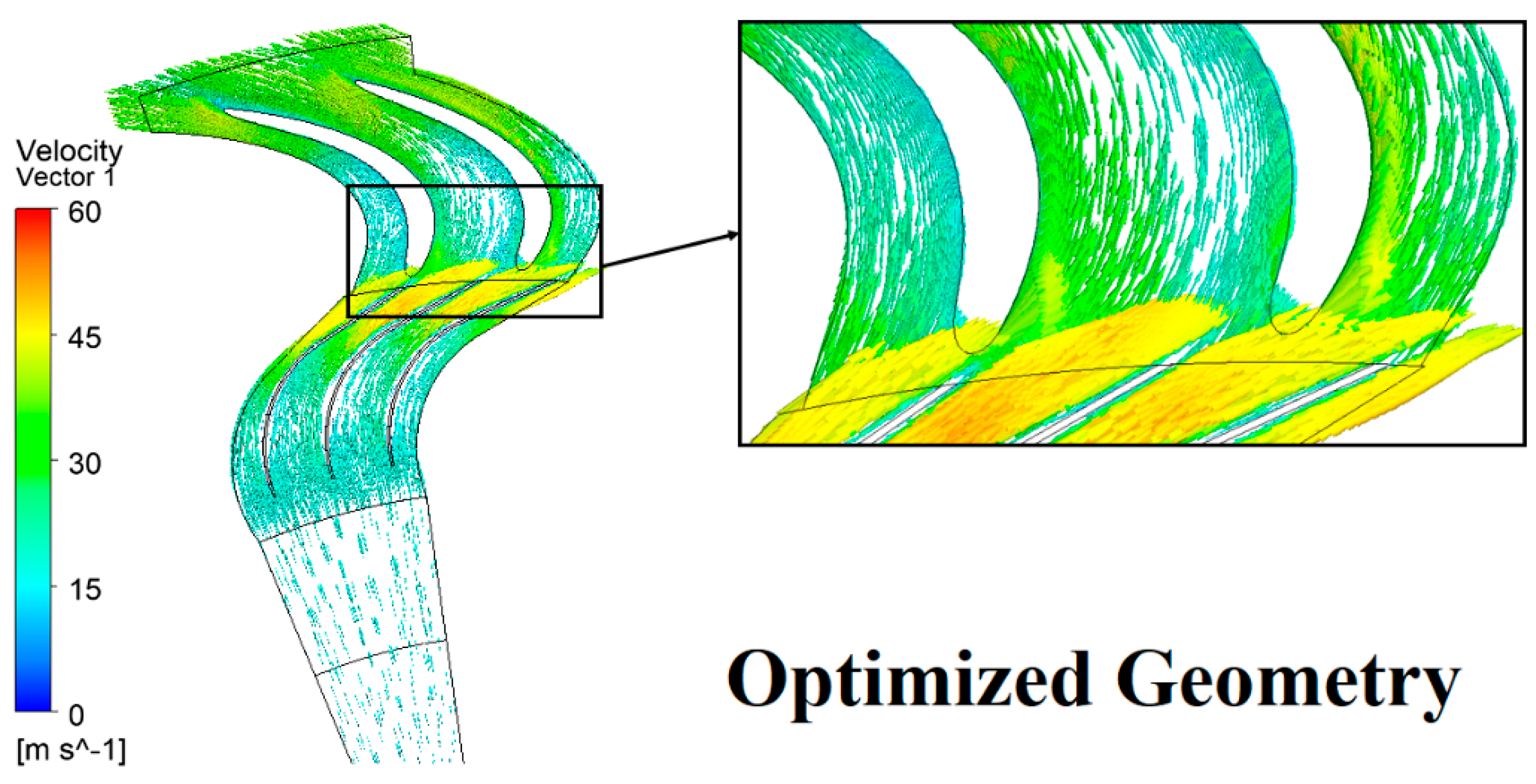
Figure 12a. It can be noted from the above-mentioned results that shape of the rotor blade can significantly affect the turbine’s performance including torque and the power conversion. The velocity vectors in the rotor domain of both geometries near their peak efficiency points (at
= 1400 Pa) are illustrated in
Figure 15 and
Figure 16. Comparing these figures shows that although the initial design allows more flowrate into the turbine domain, the rotor cannot efficiently convert the input power due to the energy losses in the domain. As shown in
Figure 15, there are huge incident losses at the leading-edge of the rotor blades in the initial design while there is a perfect stream of the flow in the turbine domain of the optimised design (
Figure 16). It can be noted that the well-matched configuration of the rotor blades with respect to the upstream guide vanes is the main reason for low flow incidence in the optimum design.
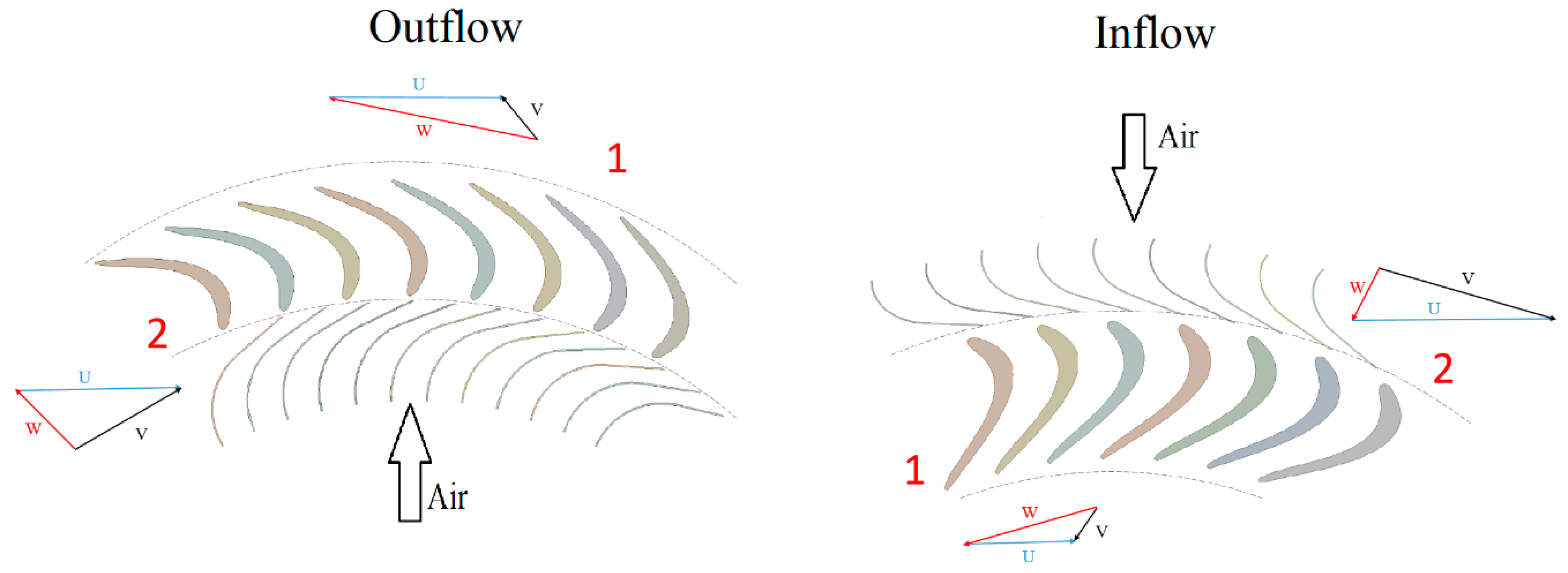
6.2. Energy Transfer in Radially Outward and Inward Flow Turbines
The Euler turbine equation can be written as the summation of energy transfer terms. These energy terms are the change in dynamic energy (associated with absolute velocity), change in centrifugal energy (associated with blade speed) and change in relative kinetic energy (associated with relative velocity) [
49]:
Here and are the absolute and relative velocities of the fluid, respectively. is the blade speed and is calculated by multiplying the blade mean radius with the blade rotational speed (ω). Subscript 2 refers to fluid entering the rotor and subscript 1 is flow leaving the rotor.
In a radially outward flow machine, due to changes in radius of rotation,
is less than
, this configuration is usually used for pumps and compressors to increase the static head. Nevertheless, an outward flow radial configuration was investigated in this research to be employed as a turbine. This design was optimised to have a maximized efficiency and its energy transfer capability will now be compared against a previously optimised inflow turbine design [
34]. The inflow turbine has 73 guide vanes at the upstream, 34 guide vanes at downstream and 51 rotor blades, more details of this turbine can be found in [
34].
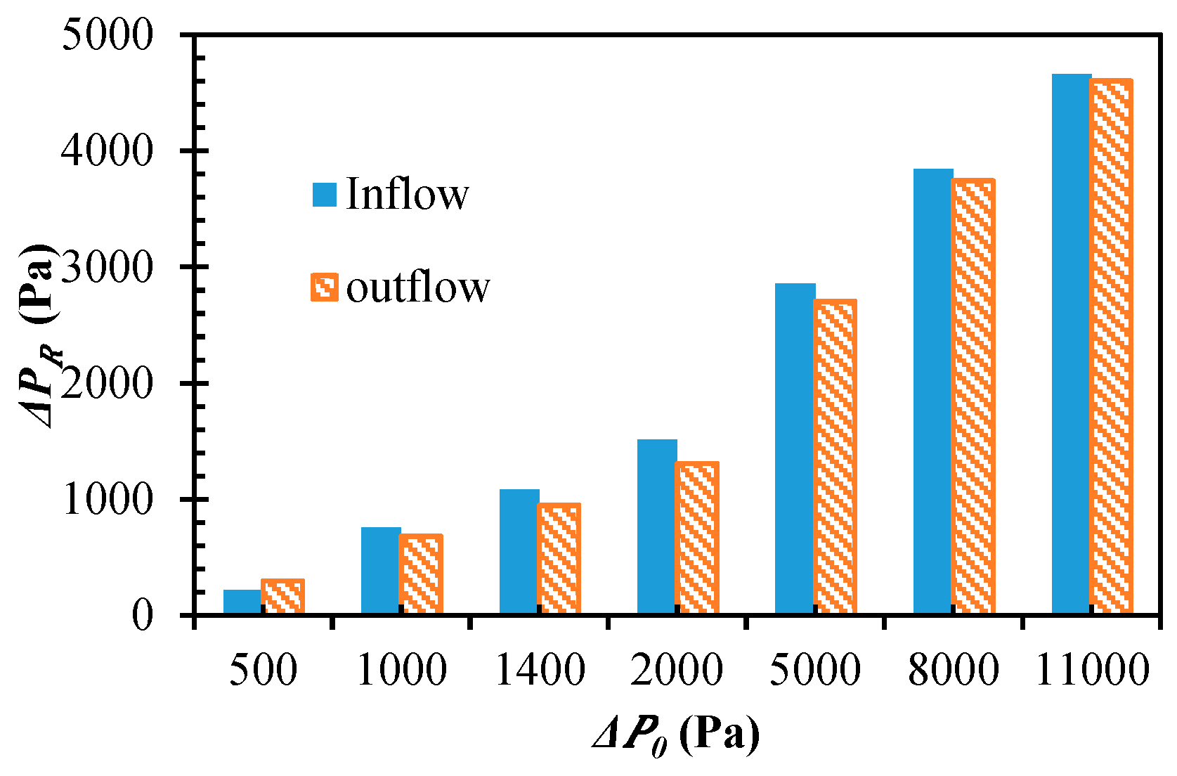
Figure 17 schematically illustrates both rotors with arbitrary angles at the entry and exit. In addition, the efficiency plots and the total pressure changes across the rotor (
) of both configurations are shown in
Figure 18 and
Figure 19, respectively. The total pressure change across the rotor was evaluated using using [
50]:
As
Figure 18 and
Figure 19 illustrate, the performance plot of the outflow turbine is comparable to that of the inflow turbine. Also, the total pressure across the outflow rotor is very close to that of the inflow rotor over the whole range of turbine pressure drops.
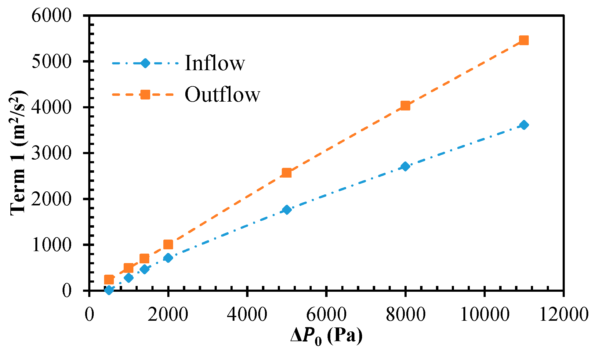
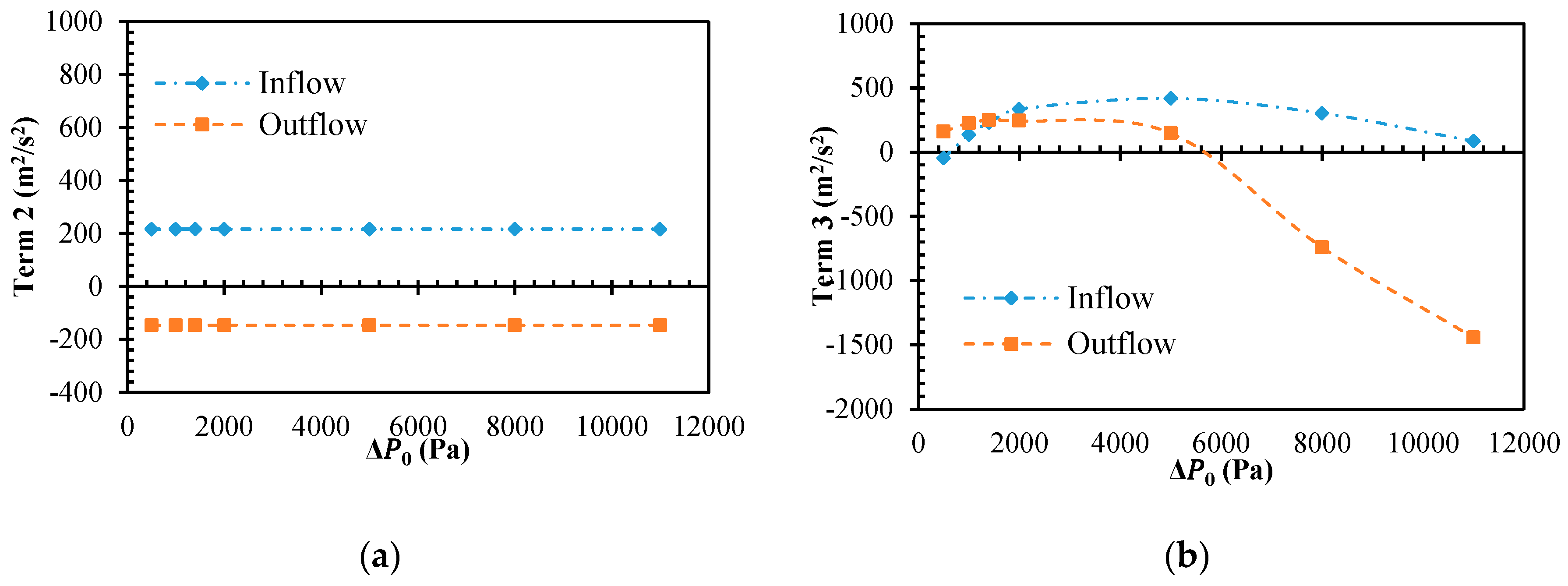
To investigate the inflow and outflow turbine configurations in further details, three terms of the energy transfer associated with changes in absolute velocity, blade speed and relative velocity are defined as
Comparison of
is illustrated in
Figure 20, which shows that the outflow turbine provides a higher change in absolute kinetic energy compared to the inflow turbine over the whole range of pressure differentials. It can be described by the geometrical features of the outflow turbine, which causes a higher change in dynamic pressure across the rotor. A comparison of the air absolute velocity at the inlet and outlet of each rotor is shown in
Figure 21, which shows higher absolute velocities of the outflow turbine design compared to the inflow turbine. As illustrated in
Figure 22a,
refers to the change in centrifugal energy is constant for each turbine. This term is negative for the outflow turbine due to the change in radius for the flow direction.
(
Figure 22b) is the change in relative kinetic energy which initially increases by the raise of pressure drop, peaks in the middle range and then reduces at high-pressure drop values. Compared to the inflow configuration, the outflow turbine has a faster response to variations of this velocity component and reaches negative values at pressure differentials higher than 6000 Pa. Generally,
affects the change in dynamic pressure through the machine, while
and
affect the static pressure changes across the rotor. It was found from this analysis of the outflow turbine that, although,
negatively affects the energy transfer, the improvements of
and
compensate for the negative portion and provide acceptable total pressure across the rotor for the specified operational range of this study.
6.3. Unsteady Performance Evaluation of the Optimum Outflow Turbine
As mentioned in
Section 3, the optimisation study was performed using a steady computational model to reduce the time and computational cost. However, the actual condition is unsteady since the computational geometry includes rotating domains. Thus, a transient model (TR) was used to control the relative motion of the rotor in a purely unsteady fashion and to evaluate the accuracy of the obtained efficiency results in the optimisation study. The steady model is called case 1, which was set up using a moving reference frame (MRF) approach and was validated in
Section 4.
In the transient model, six revolutions of the periodic domain were simulated at a rotational speed of
ω = 120 rad/s, giving a total time of 0.01232 s. The residuals were set to
, and a time step study was performed considering three different cases. Courant number (CFL) was utilised to choose a suitable time step, and it was less than one for each cell to have numerical stability [
51,
52]. First, the time step was set on
s, giving a total number of 24-time steps (this setup is referred to as case 2). Second, a time step of
s, giving a total number of 123-time steps (case 3). Finally, a time step of
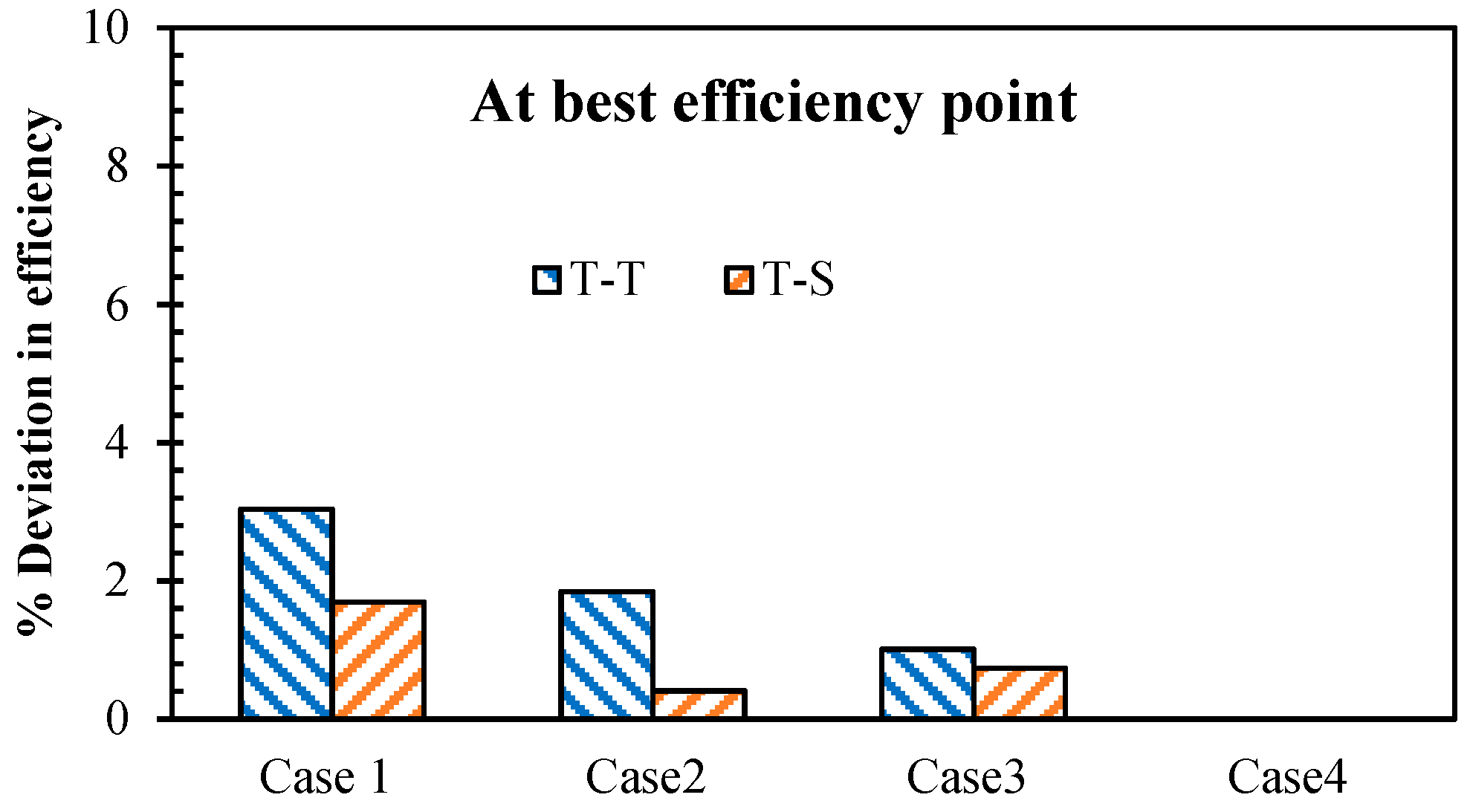
s, with a total number of 1232-time steps (case 4), this case was not economical regarding the simulation time and was used as a reference to evaluate the accuracy of other cases.
Figure 23 compares the deviation of the total to total efficiency (
) and total to static efficiency (
) of the optimum outflow turbine at its best efficiency point, obtained from cases 1 to 3 with respect to the results of case 4. According to
Figure 23, case 3 shows minor deviation from the case 4 (1% in
and 0.73% in
) but is more economical in terms of the computational cost. Therefore, case 3 with the time step of
was selected as the final transient model to simulate the optimum outflow turbine’s efficiency in an unsteady fashion. In addition,
Figure 23 shows that there is a 2% deviation in the
and less than 1% deviation in the
of the MRF model (case 1) and the transient model (case 3) at the maximum efficiency point.
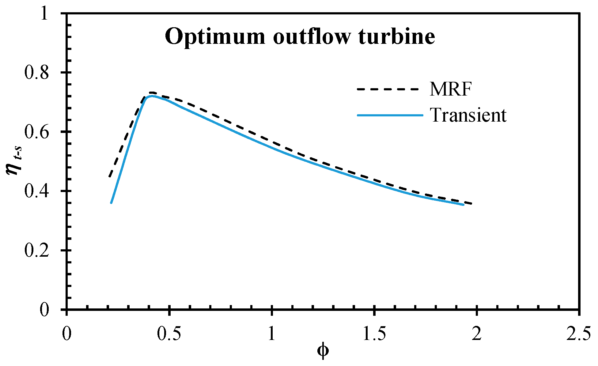
As the main concern of this study, the plot of the total to static efficiency (
of the optimum outflow turbine over the entire flow coefficient is compared for the MRF and the transient model in
Figure 24. It is obvious that the efficiency plots in both models follows a similar trend, and the steady model (MRF) has slightly overestimated the efficiency of the turbine for the whole flow coefficients. Considering the volume of the computations in the optimisation studies, benefits of using the steady model in this study strongly outweigh the 2% discrepancy and the MRF model can be regarded as an accurate model.
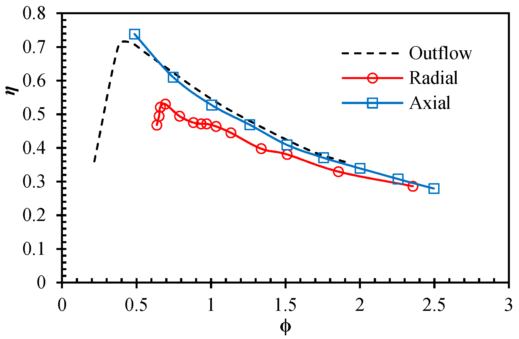
The performance of the optimised outflow turbine, obtained from the transient model, was compared to the existing unidirectional axial and radial turbines (in their direct mode) in the literature [
16,
22]. As
Figure 25 illustrates, the outflow turbine has a peak efficiency of 71%, which has a 21% improvement compared to the radial geometry suggested in [
22]. It should be noted that the radial turbine in [
22] is design-optimised to work in a twin-turbine OWC concept, when maximum efficiency in the direct mode and maximum backflow prevention in the reverse mode are desired. However, this comparison highlights that a peak efficiency of over 70% can be expected for this type of turbine, by focusing on the design optimisation to a single flow direction. The optimum outflow turbine also provides comparable efficiency to the axial turbine (the axial turbine with optimum solidity in the direct mode) in [
16], with almost 2% lower peak efficiency and slightly narrower operational range.
7. Conclusions
A design optimisation study was performed to maximize the total to static efficiency of a centrifugal radial turbine (also called outflow turbine). Seven CAD parameters were used as the design variables and their effects on the turbine performance were analysed. The optimum outflow turbine obtained 30% higher efficiency than the reference geometry. Although changes to a combination of parameters have led to the optimum turbine geometry, the LE angle was found to be the most sensitive parameter, followed by the GV angle, TE angle and the chord length. Therefore, from the point of view of the authors, including these parameters in future optimisations can lead to a more accurate exploration of the optimum rotor design. The performance of the optimum outflow turbine was evaluated in a transient model and close results were obtained compared to the MRF model. This comparison revealed that using the steady model to conduct the optimisation studies of this research was a reliable approach with a lower computational cost.
The energy transfer of the optimum centrifugal turbine was compared to an optimum centripetal alternative. It was found that change of the rotor radius causes a negative centrifugal energy transfer, however, this configuration provides a significant change of the dynamic pressure across the rotor. Thus, the total pressure changes across the turbine maintained comparable efficiency to that of a previously optimised centripetal inflow radial turbine.
The optimised outflow radial turbine obtained 72% peak efficiency (in steady-state), highlighting its comparability with the unidirectional axial alternatives in the field. There are other parameters that can affect the shape of the rotor and the flow passage between two rotor blades such as the number of rotor blades and solidity. These parameters were not included in the list of input parameters of this research. Thus, it is recommended to investigate their potential effects on the efficiency of the turbine and the turbine-chamber interactions.


