1. Introduction
This papers deals with stator current control of Induction Machines (IM) with more than three phases. It is well known that Model Based Predictive Control (MBPC) can be applied for this task in a configuration where the controller directly commands the inverter without modulation techniques [
1]. This control scheme is a particular case of the more general Finite State Model Predictive Control and is often referred to as Predictive Current Control (PCC) [
2,
3,
4]. Recently, PCC has received increasing attention as an interesting choice for multi-phase and/or multi-level systems.
One of the key aspects of MBPC is the possibility of handling constraints directly [
5] and, thus, the PCC could benefit from the constraint-handling capability of MBPC, however in most reported cases this possibility is not used. Instead, the usual practice is tuning the controller to achieve the particular compromise solution [
6]. Thus, the selection of the controller parameters is made based on the expected behavior of the IM considering some operating regions. It must be recalled that in PCC the instantaneous minimization of the cost function imprints in the IM certain current waveforms that in turn produce a a certain global behavior. It is often found that such behavior contains conflicting criteria, thus PCC design should meet the underlying trade-offs [
7]. According to this, PCC tuning should translate objectives such as commutations, tracking quality, etc. to control parameters, which is not an easy task. Regarding this, several methods have been proposed to tune the MBPC for drives in a more or less automatic fashion (see [
8,
9] for a review of methods), but the constraint satisfaction is not considered.
The proposal of this paper is to change the form of the tuning problem of MBPC so that constraints are explicitly taken into account. It is shown that this can be done by considering multiple controllers that are locally optimal in a way similar to the proposal in [
10], where, by solving the optimization problem differently for each operating region, a better global behavior can be attained.
To illustrate the method, in this paper a five-phase drive is considered. The higher number of phases (compared to the standard three-phase case) provides further room for optimization, more tuning possibilities and complex trade-offs between the different figures of merit. For this application, the problem of minimizing
losses while simultaneously maintaining the switching frequency and current tracking error below some limits is considered. For other applications, other figures of merit could be used, for instance harmonic distortion in Uninterrupted Power Systems [
11], current ripple in permanent magnet motors [
12], speed in wind turbines [
13] and others.
The chosen example problem is relevant as the five-phase machine is of interest [
14] and the proposed minimization would reduce losses without compromising dynamic performance and ensuring a switching frequency adequate for the available hardware. Please notice that the strategy is applicable to other types of systems, being the five-phase IM a particularly interesting and demanding case study that requires dealing with the extra number of phases. Application to other multi-phase systems such as the six-phase IM is straightforward thanks to the vector space decomposition technique [
15].
In the next section, the basic aspects of PCC are reviewed, introducing the figures of merit that are considered in the proposal for MBPC tuning. The concept of constraint handling via local controllers is presented in
Section 3 including the partition of operating space and the local tuning method. The resulting controller is assessed in
Section 4, paying special attention to the constraint feasibility problem for the whole operating space. From these results, some conclusions are derived in
Section 5.
2. PCC for Five-Phase IM
A brief introduction to PCC is now given to ease the presentation of the proposed variation. Although the description is given for the specific case of a five-phase IM, only minor adjustment are needed for a different number of phases thanks to the state-space representation.
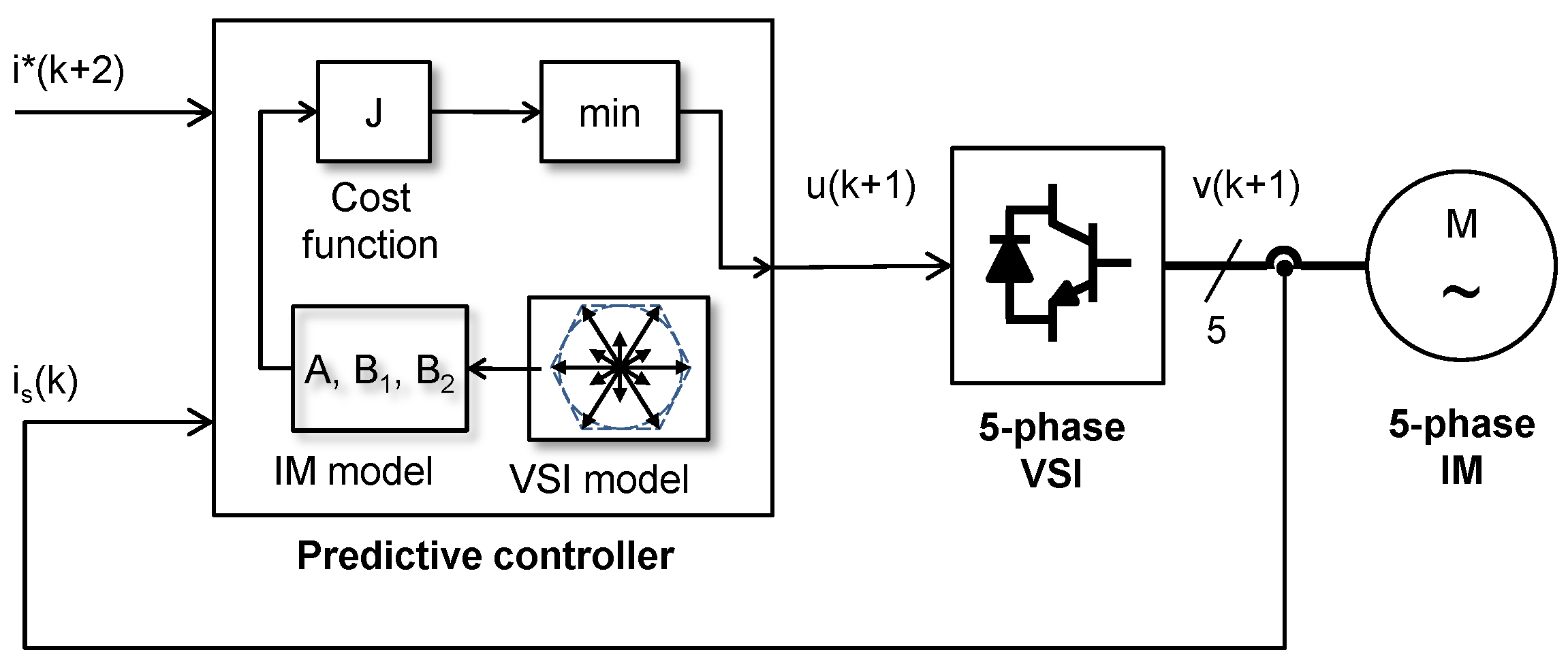
According to the block diagram of PCC shown in
Figure 1, the IM is driven by a Voltage Source Inverter (VSI) that provides a certain set of phase voltages
v that are derived from the control signal
u and the VSI topology. This produces stator phase currents
i that follow a vector of sinusoidal reference trajectories
. The PCC uses a model of the IM and VSI to predict the evolution of the stator currents associated to each possible VSI state. The controller optimizes, by exhaustive search, the control move for discrete time
, which is held for a sampling period. The procedure is then repeated according to the receding horizon rule typical of predictive controllers.
In the case of multi-phase IM with
n phases, the vector space decomposition technique provides the decomposition of the
n-phase space into one
plane, which is responsible for energy conversion and some other planes:
to
that are related to copper losses. The voltages produced by the VSI are mapped to these subspaces to form a row vector
by means of
where
is the DC link voltage,
T is a connectivity matrix that takes into account how the VSI gating signals are distributed and
M is a coordinate transformation matrix accounting for the spatial distribution of machine windings. In the case of a three-phase IM, there is no
subspace. In the case of the five-phase IM, only one auxiliary plane exists. For other multi-phase systems, the extra number of subspaces are easily treated using the state-space representation. From this decomposition, and using time-discretization, the following predictive model is obtained
where matrices
A,
and
are related to the IM electrical parameters and to the VSI connections. In addition, matrix
A is not constant but dependent on the electrical frequency
[
16]. A state space vector can be considered including stator currents in the principal and secondary planes such as
. This vector can be obtained from sensors transforming the phase stator currents
into
and
subspaces by means of the inverse transformation to that given in Equation (
1). Vector
G accounts for the dynamics due to rotor currents that are usually not measured. It constitutes a term that must be estimated at each
k [
17,
18].
In Equation (
2), the control signal
u is a vector of gating signals of the VSI
, where
for
. Each of the five phases can be connected through the VSI to the positive (
) or negative (
) borne of the DC-link. In this way, the VSI can produce
different phase voltages. Due to redundancy, only 31 different voltages are actually produced [
19].
In most applications of PCC, for discrete time
k, a value of the control signal is selected for the next sampling period
by minimizing some objective function
J. This objective function can be the sum of a number of quadratic terms penalizing control error, control effort, etc. [
5]. The simplest objective function includes the square of the predicted control error
. In the case of drives, sometimes a penalization of VSI commutations is included. This is achieved by computing the number of switch changes
produced at the VSI when the previous state
is changed to any other
as
, and the switching frequency
is
, where
is the sampling time. Please notice that the switching frequency in PCC is not constant. This drawback is a consequence of the direct digital control approach. Although this can be alleviated by using some techniques, the benefits from the elimination of the modulation stage are deemed more important in most cases. Nevertheless, the average switching frequency should not exceed some limits imposed by the VSI hardware. In addition, to limit commutation losses high values of
should be avoided. Finally, the
currents do not produce torque and are related to losses, thus it is customary to set their reference to zero. Taking these considerations into account, the cost function takes the form
where
is the vector modulus operation. It can be seen that two parameters (
and
) are needed to take into account the different scales of the variables included in the cost function. In addition, these parameters are typically used to set the relative importance of the three objectives. In a traditional PCC setup, these factors are computed off-line as a compromise between conflicting criteria and considering (in the best of cases) the whole range of operation of the system, as in [
6]. The computed values are then used on-line. This way of proceeding seems subject to potential improvement as it is realized that, for different regions of operation, the terms present in Equation (
3) take different relative values. For instance, for low speed and load, the IM shows larger harmonic distortion and lower switching frequency, whereas, for medium speed and load, the situation is the opposite [
7].
3. Constraint Handling with Local Controllers
The problem associated with constraints in PCC is that the minimization of Equation (
3) does not guarantee a certain quality of tracking or a certain commutation rate. This is because the minimization of Equation (
3) takes place at each sampling time without regard the choices made in previous periods. A possible path to overcome this would be determining a set of controller parameters (
and
) to attain the desired behavior. The following optimization problem can then be used
where
is the generic element of the search space,
is the root mean squared error obtained for tracking of
stator currents,
is the root mean squared error obtained for regulation of
stator currents, and
is the highest recorded value for the switching frequency
.
With this design procedure a minimization of
related losses is sought ensuring at the same time that the tracking error is below some limit
and that the VSI would not exceed a limit
set on the switching frequency
. Unfortunately, this problem, in general, not solvable for all operating regimes because no feasible solutions exist [
7]. It is shown that using locally tuned controllers it is possible to attain a solution for each operating regime.
3.1. Local Controllers
The concept of Local Controllers is similar to other well known methods such as the Self Tuning Regulator [
20] and Gain Scheduling [
21]. The original ideas of dividing a non-linear design problem into linear sub-problems have spurred many variations including the strategy known as Local Controller Networks [
22] where a set of controllers is considered instead of just a fixed one. At any given moment, only one controller from the set is allowed to act. The decision of which controller should be used is based on a handful of variables related to the current state of the system. This scheme can work provided that for each state an adequate/optimal controller can be uniquely determined. When the controllers in the set share the same structure and differ only in some parameters, the problem of controller selection becomes one of parameter selection. These parameters can be computed to be optimal in a, probably small, region of the system’s operating space. In this sense, the tuning (parameter selection) takes place locally, giving rise to the denomination of Local Tuning Parameters.
3.2. Partition of Operating Space
The selection of regions where local controllers are defined is not a trivial task in a general case. For the particular case of PCC of an IM drive, expert knowledge suggests using speed and load T as scheduling variables. Considering the range of variation of these variables for a particular IM, the operating space can be defined as where the over line indicates maximum value.
The partition of can be done in different ways, being the simpler a set of rectangular cells in the form obtained considering some increments and . For smaller increments, the obtained partition is finer enabling a higher possibility of obtaining an adequate scheduling.
Once the partition has been made, the MBPC parameters can be found via simulation for each region as will be shown next.
3.3. Local Tuning
For each cell
defined as
the controller parameters are selected as the solutions of Equation (
4). The limits can be the same for all operating points or follow some other rule. This is important as the minimization problem of Equation (
4) can have no solutions if the limits are too tight. To solve Equation (
4), an optimization algorithm linked to a simulation of the drive must be used. The five-phase IM, the VSI and the PCC are simulated using a Runge–Kutta method including the controller as a discrete-time part considering its computing times. The IM parameters are those of the real IM in the experimental setup that are used later for confirmation. A sampling time of
s has been used for the controller. This sampling time is enough for most modern digital signal processors to run the PCC code. Following the idea of locally tuned controllers, the simulation considers operation around each of the considered center of the partition of the operating space. The magnitude of changes must ensure that the operation remains inside the considered cell. The order of events have been found not to alter the results provided that the simulations contain enough data samples (i.e., they are not too short).
4. Results
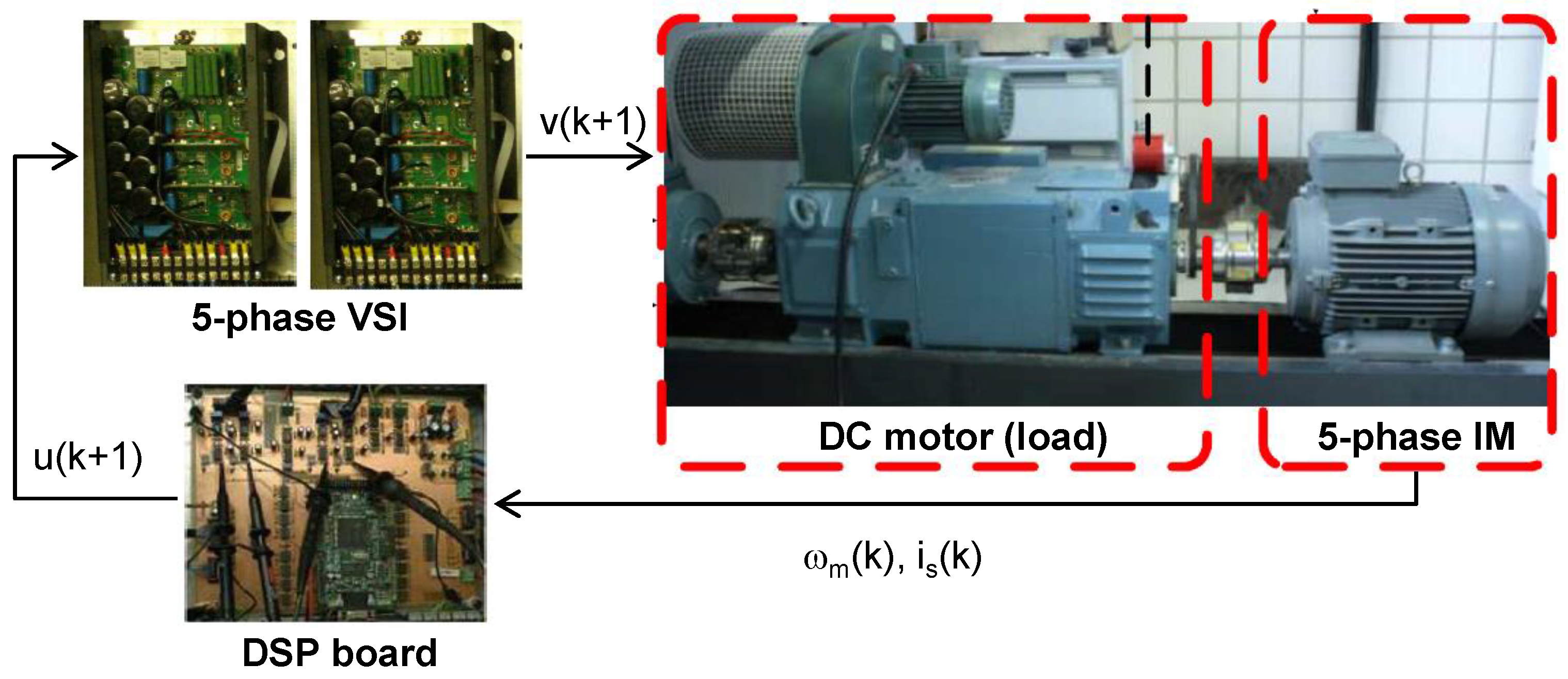
The constraint satisfaction capability of the proposed controller is assessed using computer simulations and laboratory tests in the experimental setup shown in
Figure 2. The equipment used includes a 30-slot symmetrical five-phase induction machine with distributed windings and three pole pairs. The IM is electrically supplied by means of two three-phase two-level inverters (Semikron SKS22F modules), one of which has an unused phase. A DC-link voltage of 300 (V) is applied to both modules. The predictive controller runs on a TMS320F28335 digital signal processor embedded in a MSK28335 Technosoft board with the appropriate digital and analog input/output connections. The rotor mechanical speed is measured using a GHM510296R/2500 digital rotatory encoder. The experimental setup also includes an independently controlled DC machine that is used to produce load torque in the shaft of the IM machine. In this way, different loading conditions can be tested. The electrical parameters (inductances and resistances) have been identified through experimentation, as explained in [
23], and are shown in
Table 1.
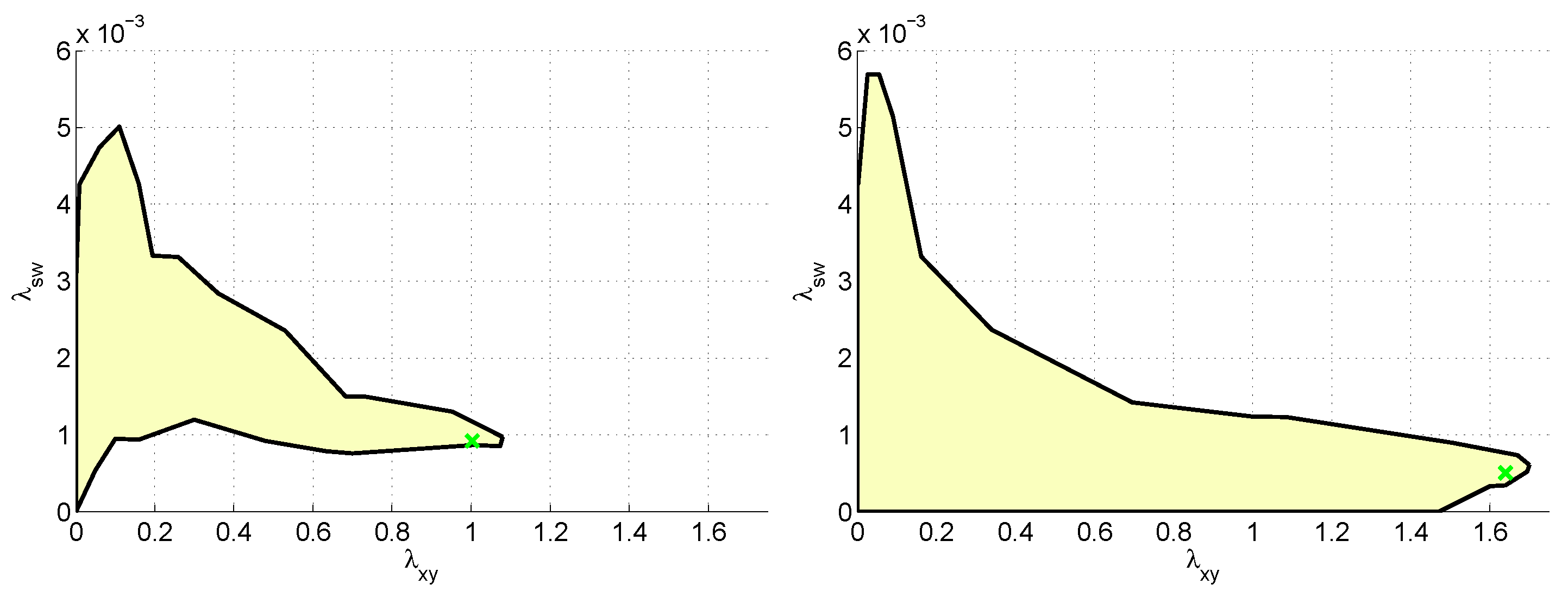
In
Figure 3(left), the feasible region for
(A),
Hz is shown for an operating point with nominal speed and load. The solution of Equation (
4) is indicated with a times mark (×) corresponding to
,
. It can be seen that the optimal solution is close to the edge of the feasible region as it usually happens in constrained optimization problems. Another example is presented in
Figure 3(right) where the operating point is characterized by low speed and load (about 30% of nominal value). Please note that the low speed zone is challenging due to the apparition of large
currents [
24]. In this case, the solution of Equation (
4) takes place for
,
. It can be seen that the optimal parameters are quite different for the two operating points considered, even if the admissible limits
U are not changed.
The same procedure is repeated for a partition of the operating space, producing an optimal value for the
parameters that characterizes the optimal controller for each cell. In
Table 2, the results are shown for a partition of moderate size (
). Please note that, for finer partitions, better results can be expected at the cost of more experimentation needed to obtain the local parameters. The acceptable limits are set as in the previous case as
(A),
Hz. The rows and columns in
Table 2 are the indices
that define the cell as
with
(rmp) and
(A). The values inside each cell are the pair
. It can be seen that the optimal values of
lie in the interval
meaning that the higher value is an order of magnitude larger than the lower. Similarly, for
, the interval is
. In addition, a nonlinear and not obvious relationship between both parameters is appreciable.
Controller Assessment
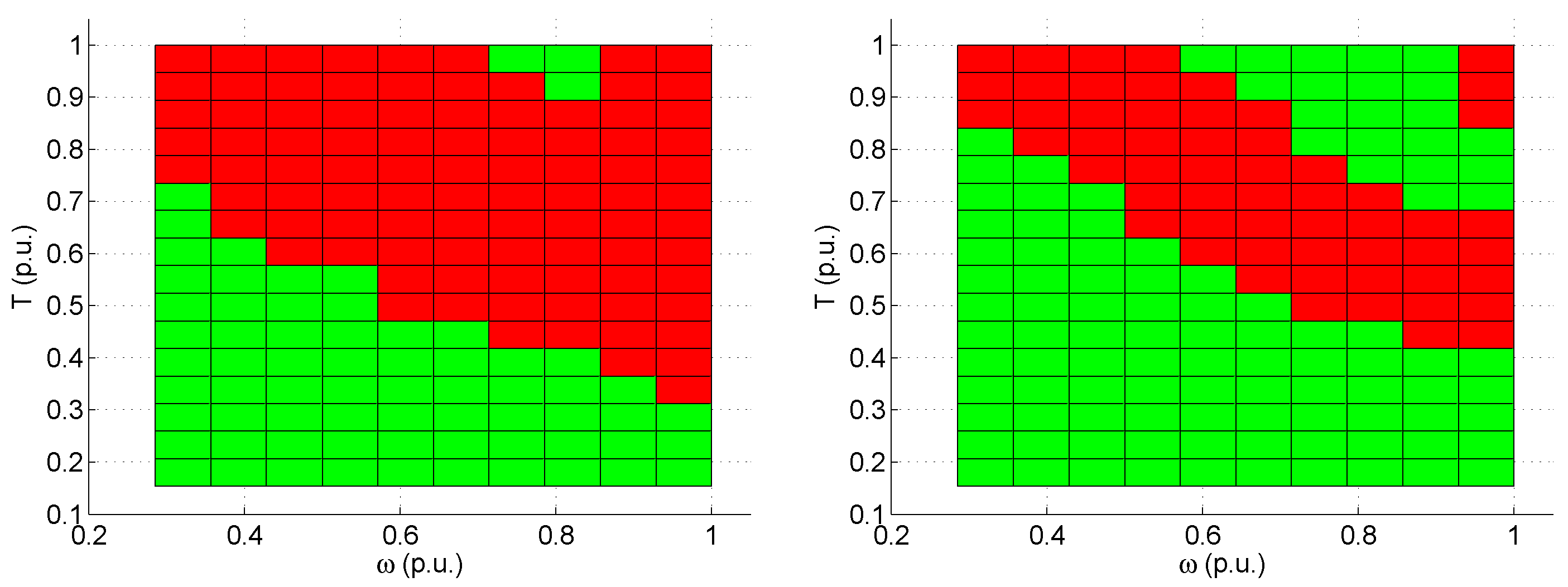
To assess the proposed scheduled PCC, a comparison with the traditional PCC is made. Several points covering the whole operating space have been considered. For each operating point, the constraints satisfaction is tested by checking the inequalities
and
. The results are presented with the help of the graph in
Figure 4, where red color is used to indicate constraint violation and green for constraint satisfaction. The left graph (Case A) is for
,
which is used in a variety of publications [
6,
23]. The graph on the right (Case B) is obtained for
,
. For the proposed strategy of scheduled local parameters, all points satisfy the constraints and thus no graph is needed.
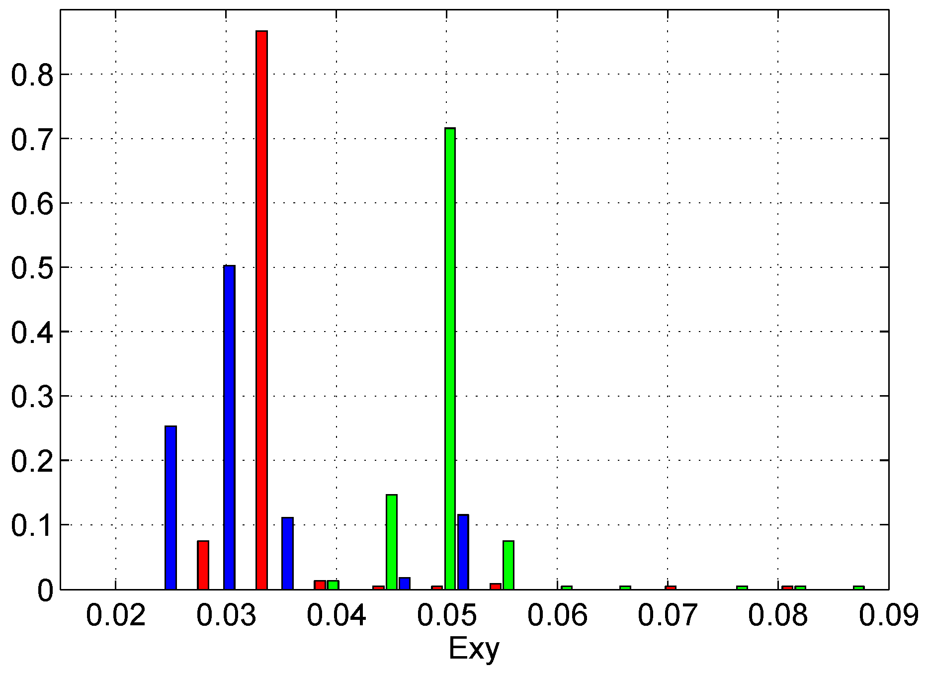
The minimization of
is now checked.
Figure 5 shows the histograms of
for the two fixed controllers (Cases A and B above) and for the proposed scheduled PCC using for each operating point the value of
indicated in
Table 2. Please note that in the histogram all points are considered and not just on the green zone (where constraints are satisfied). It can be seen that the proposed controller provides the most adequate distribution of
values, being placed at the lower end of the range. This comes in addition to meeting the constraints for all operating points, as already discussed. It is also interesting to note that Case A is better than Case B in terms of
but its region of constraint satisfaction is more limited than that of Case B, as previously shown.
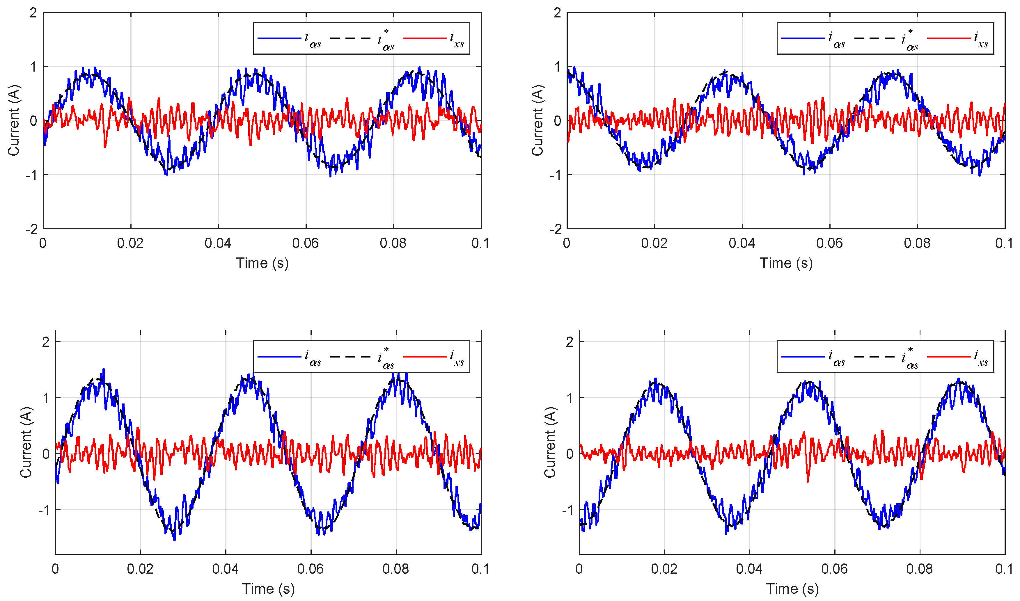
An experimental comparison of the proposed locally tuned controller with a traditional PCC with fixed weighting factors is now presented.
Figure 6 shows the trajectories of stator currents in
and
x axes (similar results are logically obtained for
and
y axes), along with the reference for
currents (for
x currents the reference is zero as
subspace generates only losses). Two operation points are considered: top row is for nominal speed and low load (Case A) and bottom row for nominal speed and 50% external torque (Case B). The tuning has been performed in this case to achieve tracking error below
(A) and a low commutation rate below
kHz. The tuning for the fixed weights PCC is found to be
,
. The locally tuned controller uses
,
for Operating Point A and
,
for Operating Point B. From the results shown in
Figure 6, it is clear that the extra degrees of freedom offered by the local tuning is exploited to obtain better tracking and less
content without violating the constraints.


