Electric Vehicle Charging Load Forecasting: A Comparative Study of Deep Learning Approaches

 , , ,
, , , 
Abstract
:1. Introduction
2. Literature Study
3. The Deep Learning Based PEV Charging Load Forecasting Framework
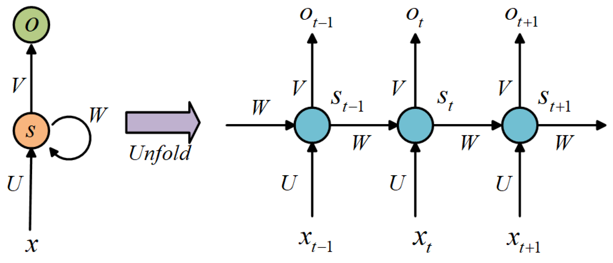
3.1. RNN Model
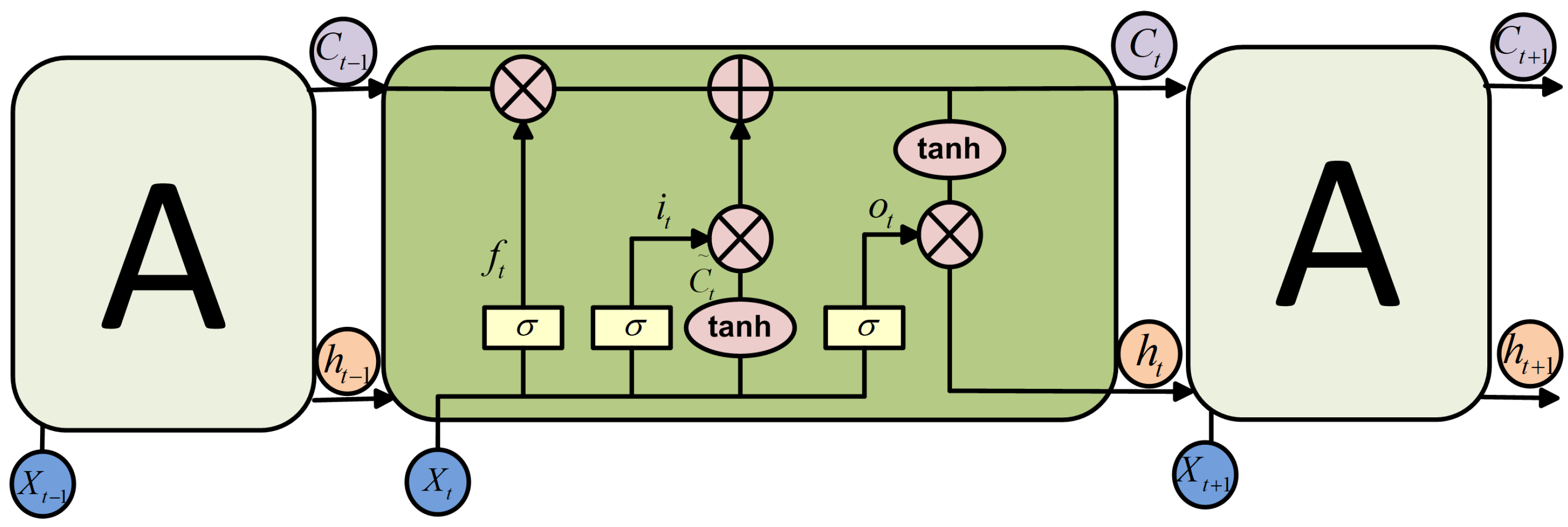
3.2. LSTM Model
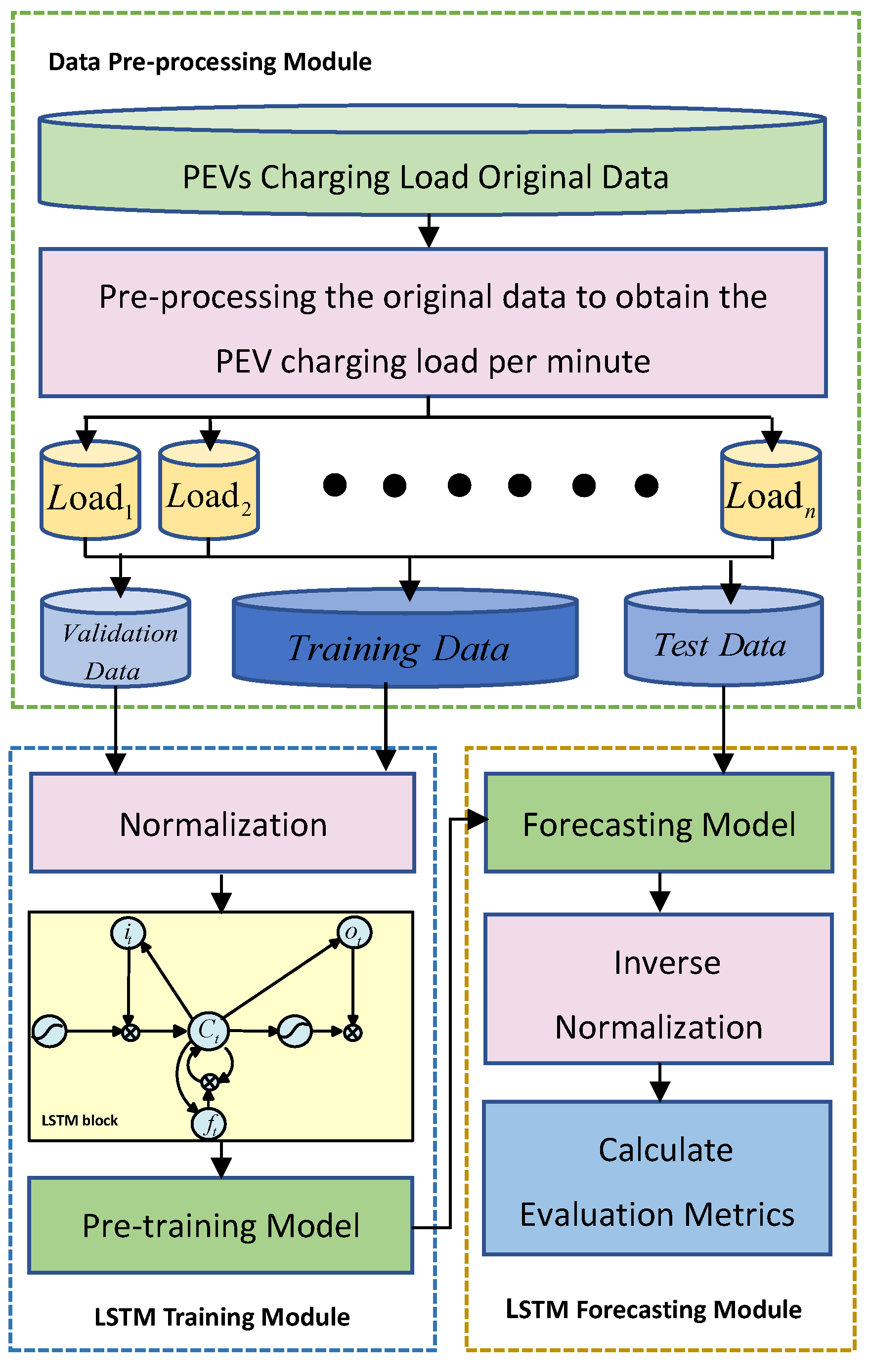
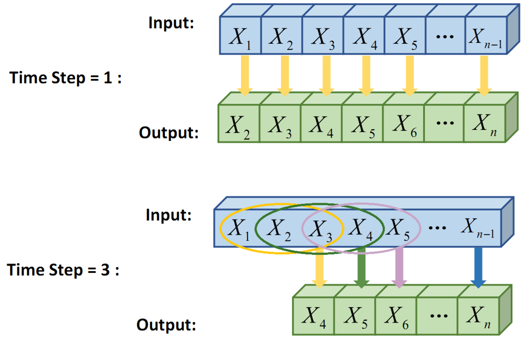
3.3. The LSTM Based PEV Charging Load Forecasting Framework
4. Data Analysis
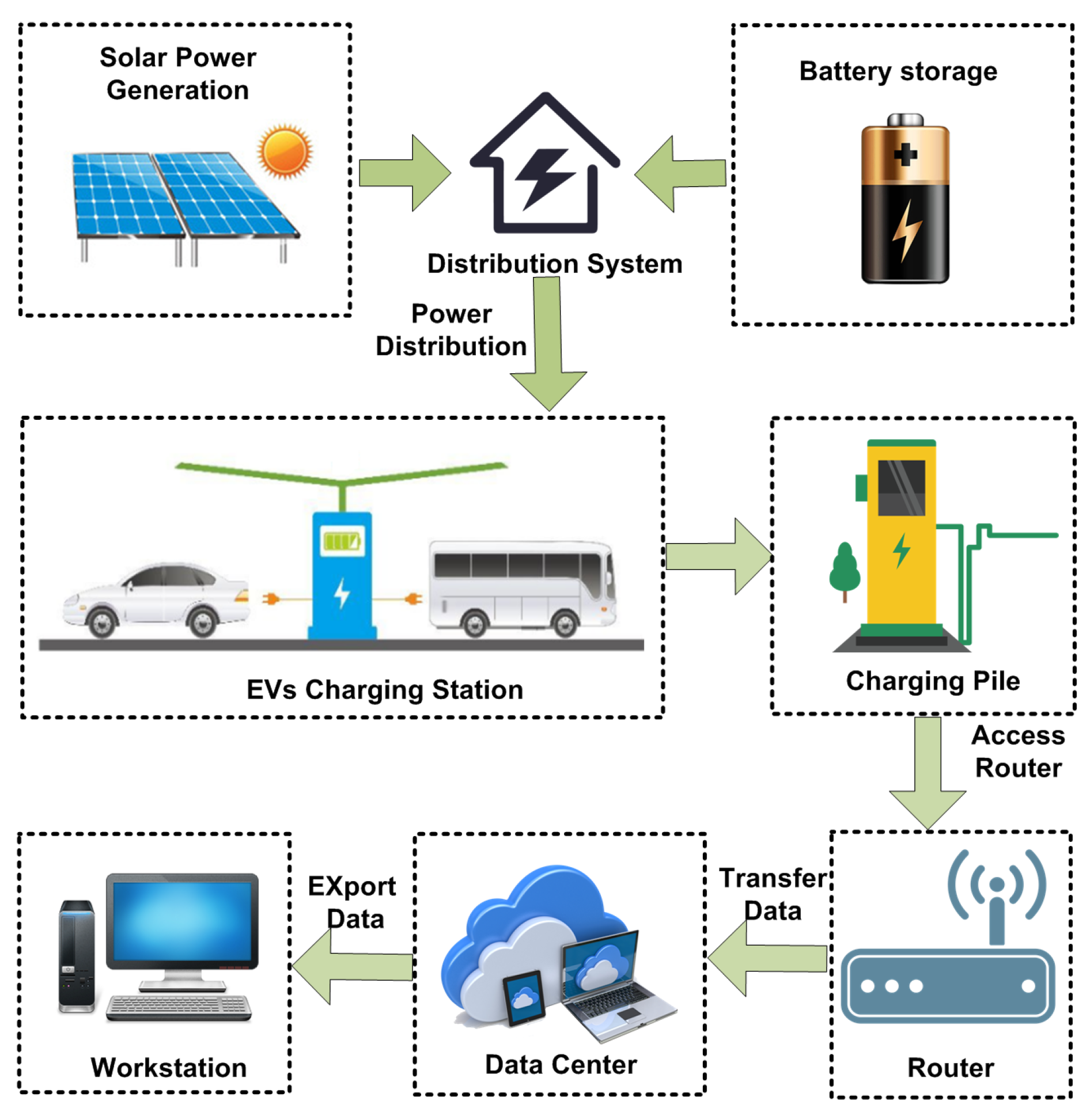
4.1. Data Statistical System
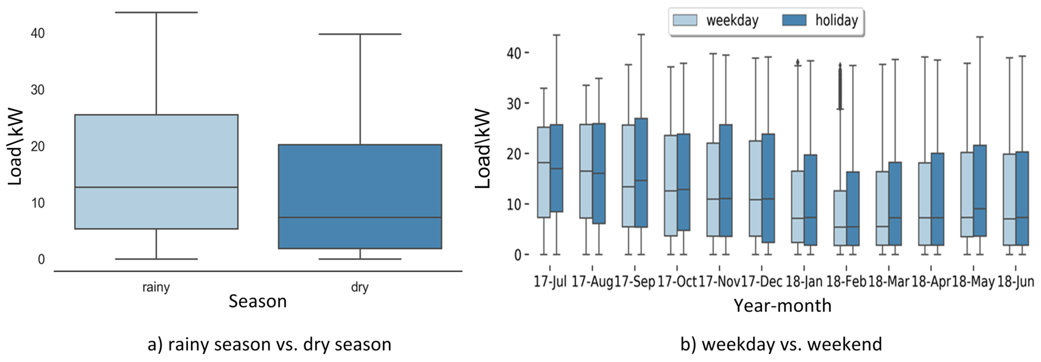
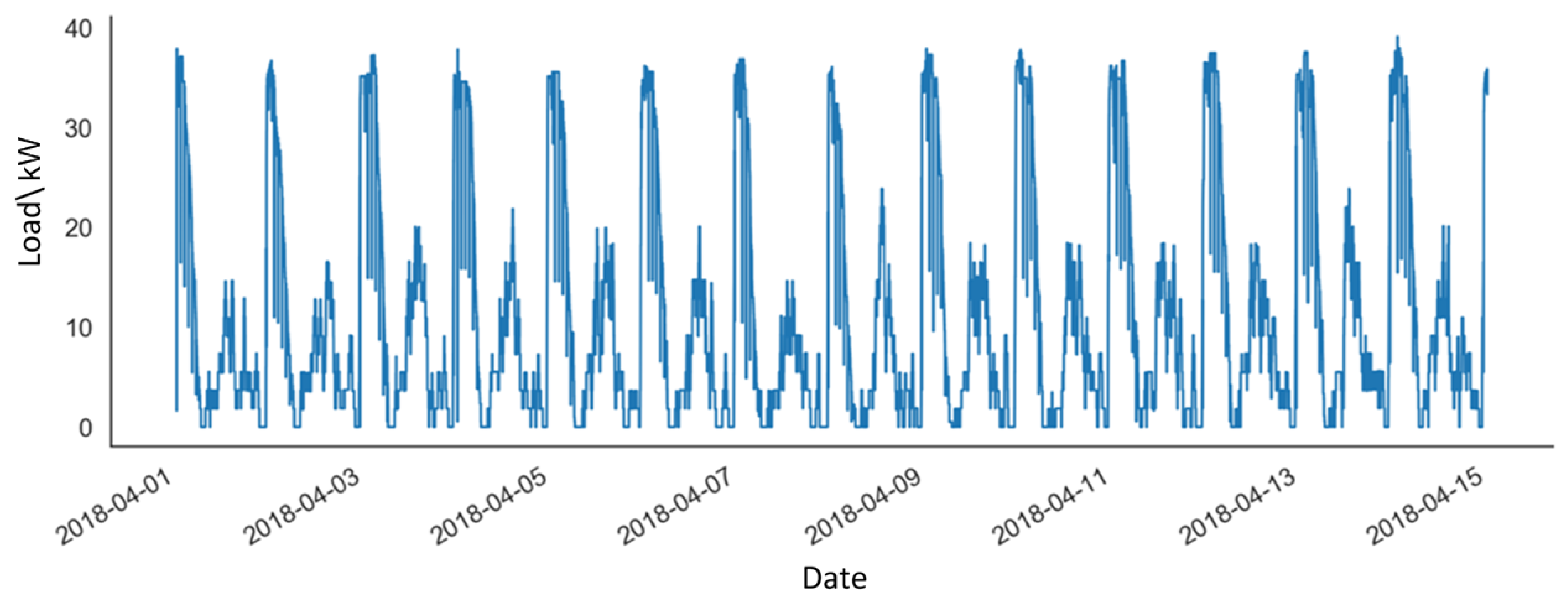
4.2. Data Pre-Processing and Feature Analysis
5. Numerical Results for Case Study
5.1. Evaluation Metrics and Error Function
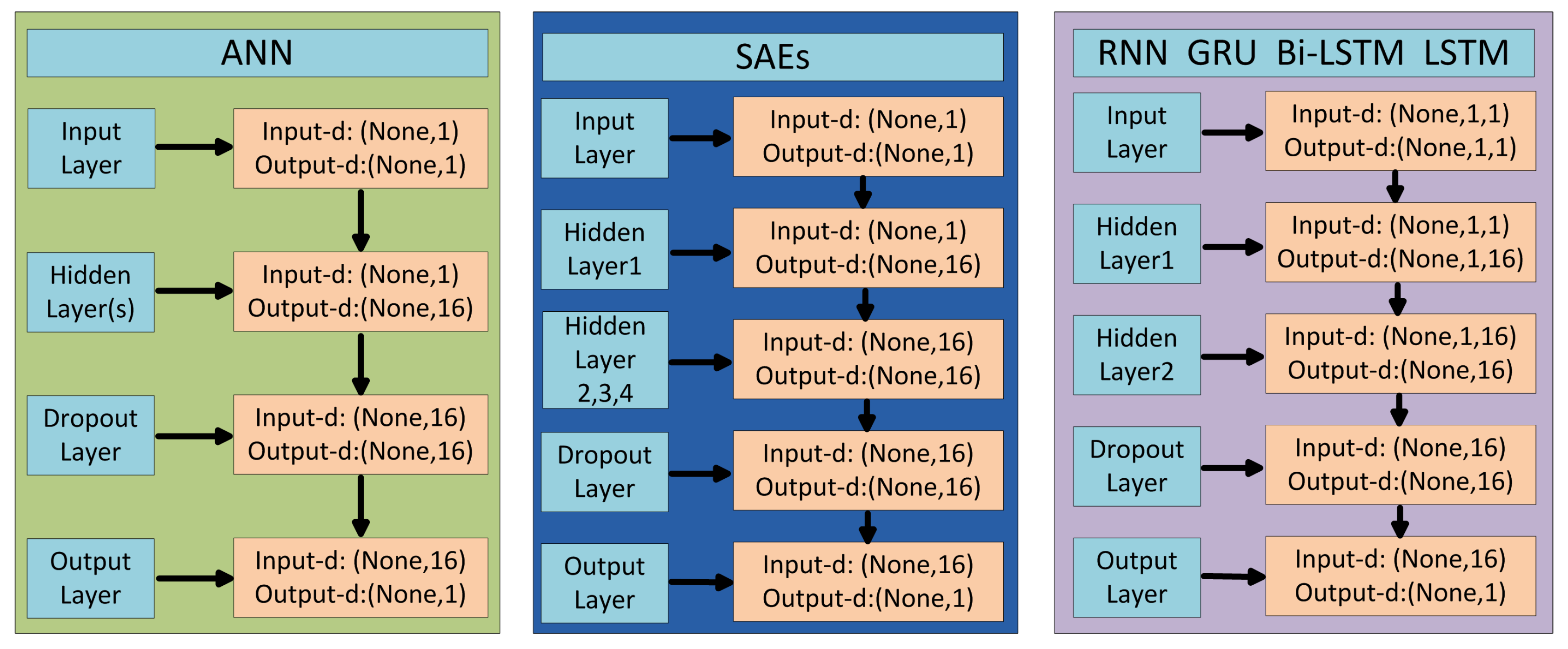
5.2. Experimental Setup
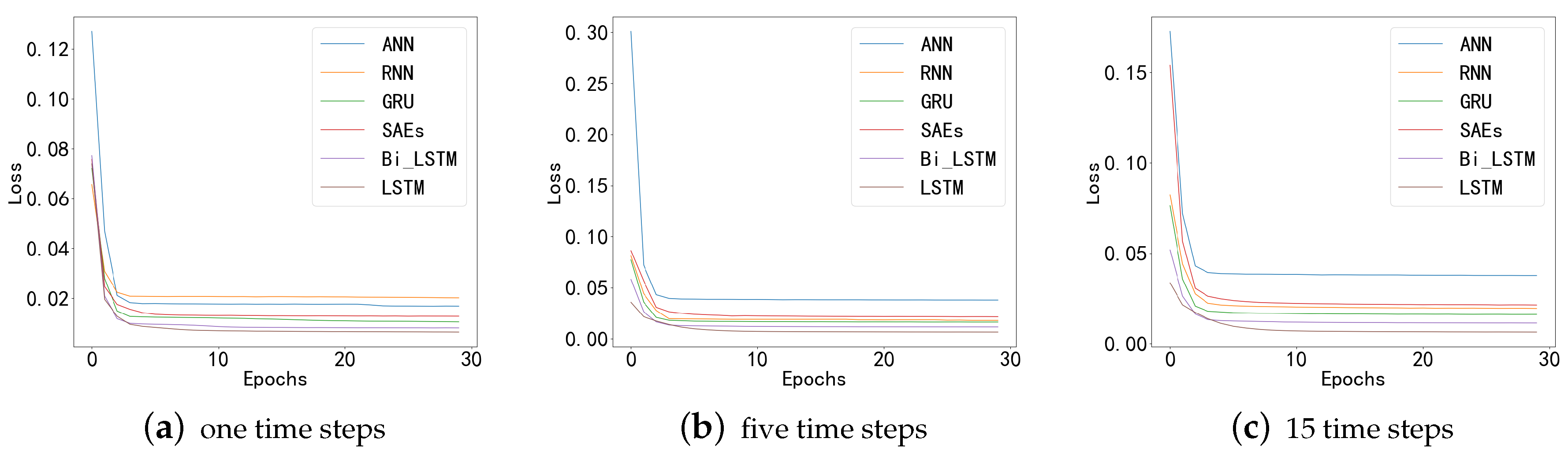
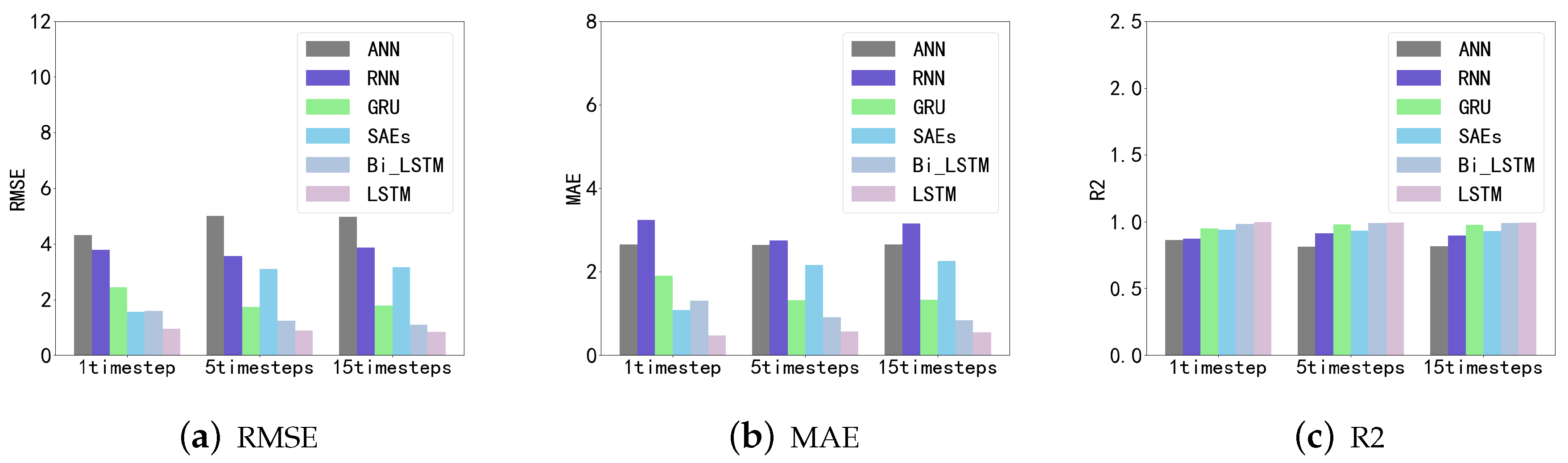
5.3. Case 1: PEV Charging Station Case Study
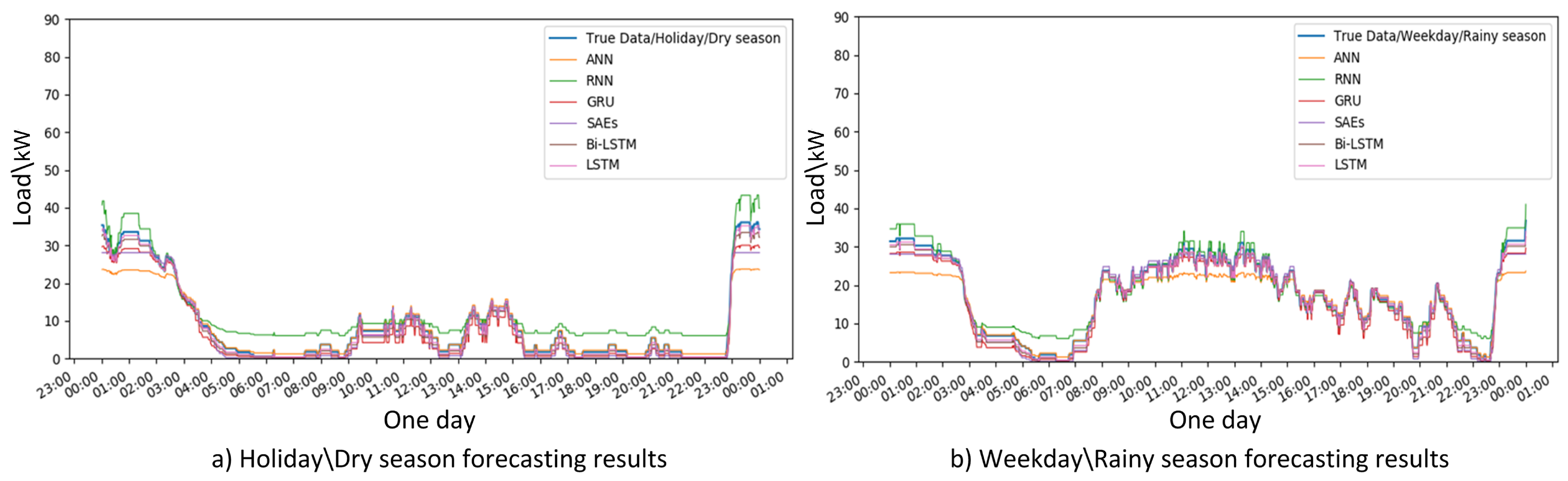
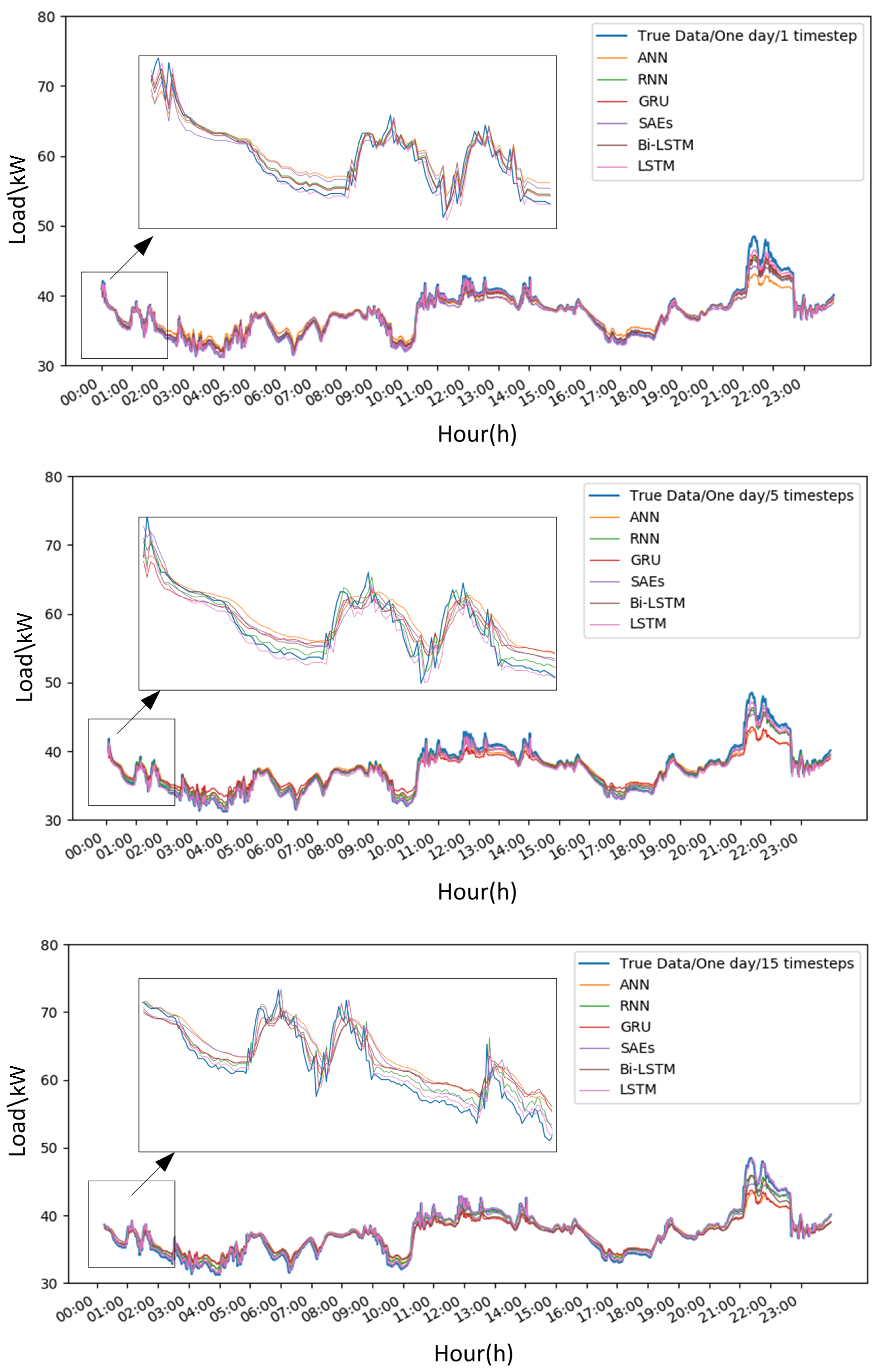
5.4. Case 2: PEV Aggregator Case Study
6. Conclusions and Future Work
Author Contributions
Funding
Acknowledgments
Conflicts of Interest
References
- Raza, M.Q.; Khosravi, A. A review on artificial intelligence based load demand forecasting techniques for smart grid and buildings. Renew. Sustain. Energy Rev. 2015, 50, 1352–1372. [Google Scholar] [CrossRef]
- Taylor, J.W. An evaluation of methods for very short-term load forecasting using minute-by-minute British data. Int. J. Forecast. 2008, 24, 645–658. [Google Scholar] [CrossRef]
- Yang, Z.; Li, K.; Foley, A. Computational scheduling methods for integrating plug-in electric vehicles with power systems: A review. Renew. Sustain. Energy Rev. 2015, 51, 396–416. [Google Scholar] [CrossRef]
- Zhang, C.; Yang, Z.; Li, K. Modeling of electric vehicle batteries using rbf neural networks. In Proceedings of the 2014 International Conference on Computing, Management and Telecommunications (ComManTel), Da Nang, Vietnam, 27–29 April 2014; pp. 116–121. [Google Scholar]
- Box, G.E.; Jenkins, G.M.; Reinsel, G.C.; Ljung, G.M. Time Series Analysis: Forecasting and Control; John Wiley and Sons: Hoboken, NJ, USA, 2015. [Google Scholar]
- Wei, L.; Zhen-gang, Z. Based on time sequence of arima model in the application of short-term electricity load forecasting. In Proceedings of the 2009 International Conference on Research Challenges in Computer Science, Shanghai, China, 28–29 December 2009; pp. 11–14. [Google Scholar]
- Haida, T.; Muto, S. Regression based peak load forecasting using a transformation technique. IEEE Trans. Power Syst. 1994, 9, 1788–1794. [Google Scholar] [CrossRef]
- Shankar, R.; Chatterjee, K.; Chatterjee, T. A very short-term load forecasting using kalman filter for load frequency control with economic load dispatch. J. Eng. Sci. Technol. Rev. 2012, 5, 97–103. [Google Scholar] [CrossRef]
- Park, D.C.; El-Sharkawi, M.; Marks, R.; Atlas, L.; Damborg, M. Electric load forecasting using an artificial neural network. IEEE Trans. Power Syst. 1991, 6, 442–449. [Google Scholar] [CrossRef]
- Chen, B.J.; Chang, M.W. Load forecasting using support vector machines: A study on eunite competition 2001. IEEE Trans. Power Syst. 2004, 19, 1821–1830. [Google Scholar] [CrossRef]
- Hippert, H.S.; Pedreira, C.E.; Souza, R.C. Neural networks for short-term load forecasting: A review and evaluation. IEEE Trans. Power Syst. 2001, 16, 44–55. [Google Scholar] [CrossRef]
- Long, J.; Shelhamer, E.; Darrell, T. Fully convolutional networks for semantic segmentation. In Proceedings of the IEEE Conference on Computer Vision and Pattern Recognition, Boston, MA, USA, 7–12 June 2015; pp. 3431–3440. [Google Scholar]
- Krizhevsky, A.; Sutskever, I.; Hinton, G.E. Imagenet classification with deep convolutional neural networks. In Advances in Neural Information Processing Systems; NIPS: Grenada, Spain, 2012; pp. 1097–1105. [Google Scholar]
- Girshick, R.; Donahue, J.; Darrell, T.; Malik, J. Rich feature hierarchies for accurate object detection and semantic segmentation. In Proceedings of the IEEE Conference on Computer Vision and Pattern Recognition, Columbus, OH, USA, 23–28 June 2014; pp. 580–587. [Google Scholar]
- Sutskever, I.; Vinyals, O.; Le, Q.V. Sequence to sequence learning with neural networks. In Advances in Neural Information Processing Systems; NIPS: Grenada, Spain, 2014; pp. 3104–3112. [Google Scholar]
- Yang, D.; Pang, Y.; Zhou, B.; Li, K. Fault Diagnosis for Energy Internet Using Correlation Processing-Based Convolutional Neural Networks. IEEE Trans. Syst. Man Cybern. Syst. 2019. [Google Scholar] [CrossRef]
- Dommel, H.W.; Tinney, W.F. Optimal power flow solutions. IEEE Trans. Power Appar. Syst. 1968, 87, 1866–1876. [Google Scholar] [CrossRef]
- Corpening, S.L.; Reppen, N.D.; Ringlee, R.J. Experience with weather sensitive load models for short and long-term forecasting. IEEE Trans. Power Appar. Syst. 1966, PAS-92, 1966–1972. [Google Scholar] [CrossRef]
- Hagan, M.T.; Behr, S.M. The time series approach to short term load forecasting. IEEE Trans. Power Syst. 1987, 2, 785–791. [Google Scholar] [CrossRef]
- Juberias, G.; Yunta, R.; Moreno, J.G.; Mendivil, C. A new arima model for hourly load forecasting. In Proceedings of the Transmission and Distribution Conference, New Orleans, LA, USA, 11–16 April 1999. [Google Scholar]
- Jie, W.U.; Wang, J.; Haiyan, L.U.; Dong, Y.; Xiaoxiao, L.U. Short term load forecasting technique based on the seasonal exponential adjustment method and the regression model. Energy Convers. Manag. 2013, 70, 1–9. [Google Scholar]
- Pai, P.F.; Hong, W.C. Support vector machines with simulated annealing algorithms in electricity load forecasting. Energy Convers. Manag. 2005, 46, 2669–2688. [Google Scholar] [CrossRef]
- Guo, Y.; Nazarian, E.; Ko, J.; Rajurkar, K. Hourly cooling load forecasting using time-indexed arx models with two-stage weighted least squares regression. Energy Convers. Manag. 2014, 80, 46–53. [Google Scholar] [CrossRef]
- Lahouar, A.; Slama, J.B.H. Day-ahead load forecast using random forest and expert input selection. Energy Convers. Manag. 2015, 103, 1040–1051. [Google Scholar] [CrossRef]
- Feng, Y.; Xiaozhong, X. A short-term load forecasting model of natural gas based on optimized genetic algorithm and improved bp neural network. Appl. Energy 2014, 134, 102–113. [Google Scholar]
- Kouhi, S.; Keynia, F. A new cascade nn based method to shortterm load forecast in deregulated electricity market. Energy Convers. Manag. 2013, 71, 76–83. [Google Scholar] [CrossRef]
- Mahmoud, T.S.; Habibi, D.; Hassan, M.Y.; Bass, O. Modelling self-optimised short term load forecasting for medium voltage loads using tunning fuzzy systems and artificial neural networks. Energy Convers. Manag. 2015, 106, 1396–1408. [Google Scholar] [CrossRef]
- Hinton, G.E.; Osindero, S.; Teh, Y.W. A fast learning algorithm for deep belief nets. Neural Comput. 2006, 18, 1527–1554. [Google Scholar] [CrossRef]
- Salakhutdinov, R.; Hinton, G. Deep boltzmann machines. In Artificial Intelligence and Statistics; Addison-Wesley: New York, NY, USA, 2009; pp. 448–455. [Google Scholar]
- Vincent, P.; Larochelle, H.; Lajoie, I.; Bengio, Y.; Manzagol, P.A. Stacked denoising autoencoders: Learning useful representations in a deep network with a local denoising criterion. J. Mach. Learn. Res. 2010, 11, 3371–3408. [Google Scholar]
- Hochreiter, S.; Schmidhuber, J. Long short-term memory. Neural Comput. 1997, 9, 1735–1780. [Google Scholar] [CrossRef] [PubMed]
- Marino, D.L.; Amarasinghe, K.; Manic, M. Building energy load forecasting using deep neural networks. In Proceedings of the IECON 2016-42nd Annual Conference of the IEEE Industrial Electronics Society, Florence, Italy, 23–26 October 2016; pp. 7046–7051. [Google Scholar]
- Kong, W.; Dong, Z.Y.; Jia, Y.; Hill, D.J.; Xu, Y.; Zhang, Y. Short-term residential load forecasting based on lstm recurrent neural network. IEEE Trans. Smart Grid 2017, 10, 841–851. [Google Scholar] [CrossRef]
- Zheng, H.; Yuan, J.; Chen, L. Short-term load forecasting using emd-lstm neural networks with a xgboost algorithm for feature importance evaluation. Energies 2017, 10, 1168. [Google Scholar] [CrossRef]
- Bouktif, S.; Fiaz, A.; Ouni, A.; Serhani, M. Optimal deep learning lstm model for electric load forecasting using feature selection and genetic algorithm: Comparison with machine learning approaches. Energies 2018, 11, 1636. [Google Scholar] [CrossRef]
- Aziz, M.; Oda, T.; Mitani, T.; Watanabe, Y.; Kashiwagi, T. Utilization of electric vehicles and their used batteries for peak-load shifting. Energies 2015, 8, 3720–3738. [Google Scholar] [CrossRef]
- Gerossier, A.; Girard, R.; Kariniotakis, G. Modeling and Forecasting Electric Vehicle Consumption Profiles. Energies 2019, 12, 1341. [Google Scholar] [CrossRef]
- Mu, Y.; Wu, J.; Jenkins, N.; Jia, H.; Wang, C. A spatialtemporal model for grid impact analysis of plug-in electric vehicles. Appl. Energy 2014, 114, 456–465. [Google Scholar] [CrossRef]
- Qian, K.; Zhou, C.; Allan, M.; Yue, Y. Modeling of load demand due to ev battery charging in distribution systems. IEEE Trans. Power Syst. 2011, 26, 802–810. [Google Scholar] [CrossRef]
- Alizadeh, M.; Scaglione, A.; Davies, J.; Kurani, K.S. A scalable stochastic model for the electricity demand of electric and plugin hybrid vehicles. IEEE Trans. Smart Grid 2014, 5, 848–860. [Google Scholar] [CrossRef]
- Luo, Z.; Song, Y.; Hu, Z.; Xu, Z.; Xia, Y.; Zhan, K. Forecasting charging load of plug-in electric vehicles in china. In Proceedings of the Power and Energy Society General Meeting, San Diego, CA, USA, 24–29 July 2011. [Google Scholar]
- Lu, Y.; Li, Y.; Xie, D.; Wei, E.; Bao, X.; Chen, H.; Zhong, X. The Application of Improved Random Forest Algorithm on the Prediction of Electric Vehicle Charging Load. Energies 2018, 11, 3207. [Google Scholar] [CrossRef]
- Zhu, J.; Yang, Z.; Guo, Y.; Zhang, J.; Yang, H. Short-Term Load Forecasting for Electric Vehicle Charging Stations Based on Deep Learning Approaches. Appl. Sci. 2019, 9, 1723. [Google Scholar] [CrossRef]
- LeCun, Y.; Bengio, Y.; Hinton, G. Deep learning. Nature 2015, 521, 436. [Google Scholar] [CrossRef] [PubMed]
- Werbos, P.J. Backpropagation through time: What it does and how to do it. Proc. IEEE 1990, 78, 1550–1560. [Google Scholar] [CrossRef]
- Chollet, F. Keras. Available online: https://keras.io/ (accessed on 18 November 2018).
- Abadi, M.; Barham, P.; Chen, J.; Chen, Z.; Davis, A.; Dean, J.; Devin, M.; Ghemawat, S.; Irving, G.; Isard, M.; et al. Tensorflow: A System for Large-Scale Machine Learning; OSDI: Boulder, CO, USA, 2016; Volume 16, pp. 265–283. [Google Scholar]
- Wei, Y.; Zhang, X.; Shi, Y.; Xia, L.; Pan, S.; Wu, J.; Han, M.; Zhao, X. A review of data-driven approaches for prediction and classification of building energy consumption. Renew. Sustain. Energy Rev. 2018, 82, 1027–1047. [Google Scholar] [CrossRef]
- Vermaak, J.; Botha, E. Recurrent neural networks for shortterm load forecasting. IEEE Trans. Power Syst. 1998, 13, 126–132. [Google Scholar] [CrossRef]
- Cho, K.; Van Merrienboer, B.; Bahdanau, D.; Bengio, Y. On the properties of neural machine translation: Encoder-decoder approaches. arXiv Preprint 2014, arXiv:1409.1259. [Google Scholar]
- Bengio, Y.; Lamblin, P.; Popovici, D.; Larochelle, H. Greedy layer-wise training of deep networks. In Advances in Neural Information Processing Systems; NIPS: Grenada, Spain, 2007; pp. 153–160. [Google Scholar]
- Graves, A.; Schmidhuber, J. Framewise phoneme classification with bidirectional lstm and other neural network architectures. Neural Networks 2005, 18, 602–610. [Google Scholar] [CrossRef]
- Tieleman, T.; Hinton, G. Lecture 6.5-rmsprop: Divide the gradient by a running average of its recent magnitude. COURSERA Neural Netw. Mach. Learn. 2012, 4, 26–31. [Google Scholar]
- Hinton, G.E.; Srivastava, N.; Krizhevsky, A.; Sutskever, I.; Salakhutdinov, R.R. Improving neural networks by preventing co-adaptation of feature detectors. arXiv Preprint 2012, arXiv:1207.0580. [Google Scholar]


| T-Step | Epoch | Loss | ANN | RNN | GRU | SAEs | Bi-LSTM | LSTM |
|---|---|---|---|---|---|---|---|---|
| 1 | 1 | Training Loss | 0.4227 | 0.1007 | 0.1067 | 0.1421 | 0.1076 | 0.0746 |
| Validation Loss | 0.1525 | 0.0253 | 0.0258 | 0.0583 | 0.0089 | 0.0136 | ||
| 10 | Training Loss | 0.0540 | 0.0270 | 0.0193 | 0.0229 | 0.0142 | 0.0079 | |
| Validation Loss | 0.0483 | 0.0169 | 0.0098 | 0.0161 | 0.0072 | 0.0048 | ||
| 20 | Training Loss | 0.0455 | 0.0271 | 0.0190 | 0.0212 | 0.0140 | 0.0070 | |
| Validation Loss | 0.0289 | 0.0166 | 0.0105 | 0.0116 | 0.0101 | 0.0033 | ||
| 30 | Training Loss | 0.0399 | 0.0271 | 0.0188 | 0.0209 | 0.0133 | 0.0068 | |
| Validation Loss | 0.0153 | 0.0149 | 0.0096 | 0.0107 | 0.0068 | 0.0031 | ||
| 5 | 1 | Training Loss | 0.3010 | 0.0810 | 0.0771 | 0.0862 | 0.0581 | 0.0356 |
| Validation Loss | 0.0793 | 0.0240 | 0.0226 | 0.0293 | 0.0156 | 0.0253 | ||
| 10 | Training Loss | 0.0382 | 0.0195 | 0.0167 | 0.0222 | 0.0118 | 0.0074 | |
| Validation Loss | 0.0185 | 0.0100 | 0.0087 | 0.0149 | 0.0067 | 0.0077 | ||
| 20 | Training Loss | 0.0380 | 0.0189 | 0.0163 | 0.0216 | 0.0116 | 0.0067 | |
| Validation Loss | 0.0196 | 0.0126 | 0.0066 | 0.0121 | 0.0052 | 0.0053 | ||
| 30 | Training Loss | 0.0378 | 0.0186 | 0.0161 | 0.0214 | 0.0115 | 0.0065 | |
| Validation Loss | 0.0196 | 0.0087 | 0.0081 | 0.0118 | 0.0055 | 0.0043 | ||
| 15 | 1 | Training Loss | 0.1726 | 0.0824 | 0.0763 | 0.1540 | 0.0519 | 0.0337 |
| Validation Loss | 0.0360 | 0.0756 | 0.0373 | 0.0509 | 0.0156 | 0.0692 | ||
| 10 | Training Loss | 0.0383 | 0.0195 | 0.0167 | 0.0224 | 0.0120 | 0.0073 | |
| Validation Loss | 0.0204 | 0.0120 | 0.0090 | 0.0129 | 0.0101 | 0.0072 | ||
| 20 | Training Loss | 0.0379 | 0.0197 | 0.0164 | 0.0217 | 0.0116 | 0.0067 | |
| Validation Loss | 0.0196 | 0.0167 | 0.0086 | 0.0120 | 0.0094 | 0.0084 | ||
| 30 | Training Loss | 0.0377 | 0.0195 | 0.0162 | 0.0214 | 0.0115 | 0.0064 | |
| Validation Loss | 0.0194 | 0.0097 | 0.0075 | 0.0115 | 0.0049 | 0.0034 |
| T-Step | Metrics | ANN | RNN | GRU | SAEs | Bi-LSTM | LSTM |
|---|---|---|---|---|---|---|---|
| 1 | MAE | 2.3582 | 3.2397 | 1.9116 | 1.0886 | 1.3096 | 0.4782 |
| RMSE | 4.3078 | 3.7915 | 2.4333 | 1.5689 | 1.5996 | 0.9546 | |
| R2 | 0.8623 | 0.8716 | 0.9495 | 0.9403 | 0.9844 | 0.9953 | |
| 5 | MAE | 3.0206 | 2.7457 | 1.3134 | 2.1616 | 0.9045 | 0.5734 |
| RMSE | 5.0117 | 3.5703 | 1.7376 | 3.1042 | 1.2288 | 0.8937 | |
| R2 | 0.8136 | 0.9104 | 0.9788 | 0.9323 | 0.9894 | 0.9944 | |
| 15 | MAE | 2.9988 | 3.1559 | 1.3269 | 2.2516 | 0.8296 | 0.5500 |
| RMSE | 4.9680 | 3.8630 | 1.7880 | 3.1556 | 1.0934 | 0.8452 | |
| R2 | 0.8168 | 0.8941 | 0.9756 | 0.9292 | 0.9916 | 0.9950 |
| T-Step | Metrics | ANN | RNN | GRU | SAEs | Bi-LSTM | LSTM |
|---|---|---|---|---|---|---|---|
| 1 | MAE | 0.9098 | 0.4751 | 0.4281 | 0.7008 | 0.5321 | 0.3096 |
| RMSE | 1.2581 | 0.6890 | 0.6340 | 0.9551 | 0.7702 | 0.5095 | |
| R2 | 0.8603 | 0.9581 | 0.9645 | 0.9195 | 0.9476 | 0.9771 | |
| 5 | MAE | 0.8912 | 0.4830 | 0.5112 | 0.5529 | 0.6241 | 0.4699 |
| RMSE | 1.2654 | 0.6761 | 0.7218 | 0.7638 | 0.8091 | 0.6219 | |
| R2 | 0.8585 | 0.9596 | 0.9361 | 0.9484 | 0.9421 | 0.9658 | |
| 15 | MAE | 0.8823 | 0.4659 | 0.6111 | 0.6576 | 0.8157 | 0.2864 |
| RMSE | 1.2489 | 0.6506 | 0.8519 | 0.8956 | 1.0260 | 0.4418 | |
| R2 | 0.8626 | 0.9627 | 0.9284 | 0.9293 | 0.9072 | 0.9828 |
© 2019 by the authors. Licensee MDPI, Basel, Switzerland. This article is an open access article distributed under the terms and conditions of the Creative Commons Attribution (CC BY) license (http://creativecommons.org/licenses/by/4.0/).
Share and Cite
Zhu, J.; Yang, Z.; Mourshed, M.; Guo, Y.; Zhou, Y.; Chang, Y.; Wei, Y.; Feng, S. Electric Vehicle Charging Load Forecasting: A Comparative Study of Deep Learning Approaches. Energies 2019, 12, 2692. https://doi.org/10.3390/en12142692
Zhu J, Yang Z, Mourshed M, Guo Y, Zhou Y, Chang Y, Wei Y, Feng S. Electric Vehicle Charging Load Forecasting: A Comparative Study of Deep Learning Approaches. Energies. 2019; 12(14):2692. https://doi.org/10.3390/en12142692
Chicago/Turabian StyleZhu, Juncheng, Zhile Yang, Monjur Mourshed, Yuanjun Guo, Yimin Zhou, Yan Chang, Yanjie Wei, and Shengzhong Feng. 2019. "Electric Vehicle Charging Load Forecasting: A Comparative Study of Deep Learning Approaches" Energies 12, no. 14: 2692. https://doi.org/10.3390/en12142692
APA StyleZhu, J., Yang, Z., Mourshed, M., Guo, Y., Zhou, Y., Chang, Y., Wei, Y., & Feng, S. (2019). Electric Vehicle Charging Load Forecasting: A Comparative Study of Deep Learning Approaches. Energies, 12(14), 2692. https://doi.org/10.3390/en12142692