An Energy-Efficient Timetable Optimization Approach in a Bi-DirectionUrban Rail Transit Line: A Mixed-Integer Linear Programming Model

Abstract

The quick growth of energy consumption in urban rail transit has drawn much attention due to the pressure of both operational cost and environmental responsibilities. In this paper, the timetable is optimized with respect to the system cost of urban rail transit, which pays more attention to energy consumption. Firstly, we propose a Mixed-Integer Non-Linear Programming (MINLP) model including the non-linear objective and constraints. The objective and constraints are linearized for an easier process of solution. Then, a Mixed-Integer Linear Programming (MILP) model is employed, which is solved using the commercial solver Gurobi. Furthermore, from the viewpoint of system cost, we present an alternative objective to optimize the total operational cost. Real Automatic Fare Collection (AFC) data from the Changping Line of Beijing urban rail transit is applied to validate the model in the case study. The results show that the designed timetable could achieve about a 35% energy reduction compared with the maximum energy consumption and a 6.6% cost saving compared with the maximum system cost.

1. Introduction

Compared to other modes of urban transport, the metro system has a larger transport capacity, high security, and is much more energy efficient [1]. Therefore, it has received rapid development around the world in recent years. For example, 36 cities in China operated the urban rail transit over 4800 km in 2018. According to the Web of China Rail Transit, there will be more than 50 cities operating urban rail transit over the next few years. In 2020, the total mileage of urban rail transit in China will reach 6000 km. However, Since the fast extension of the urban rail transit network, there has been a rapid corresponding increase of energy consumption in the urban rail transit system. This has attracted wide attention from both the environmental sectors and academic research [2]. In Beijing, as shown in Figure 1, from 2010–2017, the energy consumption of the urban rail transit system had increased two times to over 1.8 billion kWh in 2017 according to the data from Beijing urban rail transit. The enormous energy consumption generates not only huge operation cost, but also tough environmental responsibilities. The electricity cost accounts for over one-third of the total operation cost of Beijing urban rail transit, which has undertaken an energy-saving task from the Beijing government for the carbon emission requirement and sustainable development. Similarly, in the European Union (EU), metropolitan transportation is responsible for about 25% of the total CO${}_2$ emissions in the transport system [1]. Moreover, there are detailed targets for the EU to reduce CO${}_2$ emissions. More specifically, the short-term target is to reduce CO${}_2$ emissions by 30% during the preliminary period from 1990–2020, with a further reduction by 50% in 2030 [3].

Timetabling is done after the upper management stage (line planning) that determines the routes and stop schedules of the trains. The line planning is at a more macroscopic level. The timetabling is a more detailed implementation, which may be adjusted annually. A well-designed timetable will have essential influences on the scheduling staff and rolling stock, which are simultaneously determined for daily operation. The basic consideration for the timetable problem is passenger flow. The passenger will profit from a well-designed train timetable with elaborate arrival times, departure times, dwell times, and running times. However, the operation cost for the operator is of equal importance. The energy consumption is not only one main cost, but also entails responsibility for environmental protection. In this paper, we aim to design a timetable from the perspective of the system cost of urban rail transit, which pays more attention to energy consumption. Since the costs of staff and rolling stock are considered in the model, the conducting of an energy-efficient timetable will be effective in the operation.

The timetable problem consists of optimizing the arrival time, dwell time, and departure time of trains at each station on the line under the time relationship and passenger demand constraints [4]. In particular, an energy-efficient timetable pays more attention to the running process in the section, which greatly affects the energy consumption and running time. There is a long history of research (Howlett et al. [5], Yang et al. [6], Canca et al. [4], Huang et al. [7]) focusing on energy-efficient train operation. It is always solving the optimal train control problem based on the Pontryagin Maximum Principle (PMP). Therefore, it is the primary step to determine the optimal driving strategy under the Pontryagin maximum principle. However, because of the non-linearity of the train control principle, it is hard to get a precise and optimal solution when modeling the timetable problem into a non-linear formulation. Although many studies employed the non-linear model with solutions based on the heuristic methods such as the intelligent Genetic Algorithm (GA) [8], it might fall into local optima or find an approximate optimum by heuristic methods. To fill this gap, we manage to make the following contributions:

(1)

We develop an approach with a mixed-integer linear programming formulation to optimize the supplement of running time in each track, arrival time, dwell time, and departure time at each platform, which aims at reducing the total energy consumption in the planning horizon.

(2)

A mixed-integer linear programming model is proposed by linearizing the objective and constraints, and it can be solved by the modern solver (Gurobi) easily.

(3)

Then, from the perspective of the system cost, we develop an alternative objective based on the energy-efficient model, which gives an elaborate timetable for the conservation of system costs during the operation.

(4)

Moreover, real data from Beijing Changping Line is employed to validate the integrated approach, and the results are logically explained.

The remainder is organized as follows. The literature is reviewed in Section 2. Then, a mixed-integer non-linear programming model is developed in Section 3. By linearizing the objective and constraints, a mixed-integer-linear programming model is proposed in Section 4. From a system perspective, we give an alternative objective in Section 5. In Section 6, real data from Beijing urban rail transit are taken to validate the model. Finally, Section 7 gives the summaries of the results and suggestions for the future.

2. Literature Review

Energy-efficient train operations make an essential contribution to cutting down the energy consumption of the urban rail transit system [6]. There are three main types, including optimal train control, timetable optimization, and integrated optimization.

A collection of papers published after the 1990s was focused on optimal train control [9,10,11]. During the preliminary stage, Howlett (1994) [5] proposed a discrete model that considered the speed limits with fixed running time and used Kuhn–Tucker conditions to prove the optimal control strategy. Furthermore, Howlett and Cheng (1997) [12] solved the matter by applying continuously-varying gradients. Then, Khmelnitsky et al. (2000) [13] and Albrecht et al. (2013) [14] utilized independent arguments with different conditions and ensured that the optimal strategy was unique. Rodrigo et al. (2013) [15] discretized the speed profile and applied the Lagrange multipliers method to find semi-analytical solutions. Recently, aiming to find the optimal speed profiles and control regimes to cover the safety, punctuality, and energy efficiency of train operations, Wang et al. (2016) [16] studied the train trajectory optimization problem, which considered both the operational and signaling constraints. Paying attention to delay cases, with the two objectives of reducing delays and reducing energy consumption, Wang et al. (2017) [17] proposed a multi-train trajectory optimization for single-track lines. However, the traditional optimal control method is complex and needs many physical parameters of the train that were tested by the train factory. Therefore, a data-driven optimization model emerges. Huang et al. (2019) [7] proposed a Data-Driven Optimization Model (DDOM) to describe the relationship between energy consumption and the discrete speed profile, then integrated two typical machine learning algorithms, Random Forest Regression (RFR) and Support Vector machine Regression (SVR), into a heuristic algorithm to solve the model.

Similarly, much research has been associated with the train timetable optimization problem in rail transportation systems (Shakibayifar et al., 2017 [18], Wang et al., 2017 [19], Gainanov et al., 2017 [20], Hassannayebi et al., 2018 [21]). These studies have enhanced the optimization theory and practice in the timetable problem. However, the timetable problem involves many sub-problem and still needs more research. Under the constraint of providing enough frequencies with acceptable services, Hu and Liu (2014) [22] proposed a headway-oriented timetable model to optimize the cost of a mass rapid transit system. Paying attention to the coordination between the last trains at the transfer stations of the urban rail transit networks, Kang et al. (2015) [23] proposed a method to reveal the relationships between the passenger transfer connection time and passenger transfer waiting time. To prevent passenger congestion and long waiting through train scheduling, Hassannayebi et al. (2016) [24] aimed to minimize the average waiting time of the passengers by using a path-indexed non-linear model to optimize the train timetable. Under the condition of emergencies, with the purpose of achieving the minimum delay time in the urban rail network, a binary mixed-integer programming model was presented by Huo et al. (2016) [25] based on the priority and train order entropy. To stress the level of transfer synchronization in the urban rail network, Guo et al. (2017) [26] presented a mixed-integer non-linear programming model with the objective of maximizing synchronization of the transfer process, which was solved through the combined heuristic of Particle Swarm Optimization and Simulated Annealing (PSO-SA). The energy consumption was described as a diminishing function of the section’s running time. Canca and Zarzo (2017) [27] presented a mixed-integer non-linear model to optimize the timetable, which was solved using a sequential mixed-integer linear procedure. To handle the train departure orders, running time, dwell time, and overtaking locations flexibly, Sparing and Goverde (2017) [28] described an optimization method for designing a periodic timetable with the aim of finding the maximum stability within a heterogeneous railway network.

Integrated optimization in energy-efficient operations has recently become a hot issue, especially combining timetables with speed profile optimization (Zhou et al., 2017 [29], Yin et al., 2017 [30], Wang et al., 2019 [31], Gao et al., 2019 [32]). Chevrier et al., 2013 [33] proposed a multi-objective evolutionary algorithm with the objectives of finding the optimal running time and reducing energy consumption. In addition, focusing on improving the utilization of train regenerative energy through the timetable optimization has also attracted more attention (Yang et al., 2016) [6]. Taking into account the dynamic train scheduling, Li and Lo (2014) [34] developed a control framework that simultaneously forecasted passenger demand, as well as optimized the timetable and speed profile. When the transportation service operator and passenger costs were simultaneously considered in a dense passenger Railway Rapid Transit (RRT) network, a Mixed-Integer Non-Linear Programming (MINLP) model was employed by Canca et al. (2016) [4] for optimizing the frequencies and determining the capacities. Time-dependent passenger demand in oversaturated conditions was also considered with the traffic capacity constraints. Then, in the operation scenario of two trains in multiple inter-stations, Huang et al. (2018) [2] integrated the operation strategies with optimizing the train timetable in pursuit of minimizing the energy consumption. Taking multi-phase speed limits into account, Yang et al. (2018) [35] employed an energy-efficient timetable model, which determined both the timetable and speed profile in each section by Particle Swarm Optimization (PSO) methods. Then, through the Taylor approximation, they transformed the train scheduling problem using a non-convex formation into a quadratic formation. Finally, an active set method was employed to search for the approximate optimal solution. Taking into account both the passenger waiting time and energy consumption under oversaturated conditions, Sun et al. (2019) [36] presented a bi-objective model and conducted a case study using a GA search in the Beijing subway system. By introducing a stop-skipping pattern before timetable optimization, Yang et al. (2019) [37] proposed a two-step optimization-based approach, which determined the specific skipped station based on the passenger smart-card data in the first-step, then modeled the energy-efficient timetable problem in convex quadratic programming, which was solved by the CPLEX. When the abnormal condition occurred (like delay perturbations), Yang et al. (2019) [38] employed an energy-efficient rescheduling approach to minimize the net energy consumption under the premise of reducing or eliminating the delay altogether.

Based on the review above, as we know, modeling the energy-efficient timetable problem by a special linearization technique to determine the timetable and train profile simultaneously has not been considered well. Furthermore, the complex model or using the heuristic algorithm to get an approximate solution should be improved. Therefore, this research is a supplement for relevant studies.

3. The Timetable Optimization Model: Mixed-Integer Non-Linear Programming Formulation

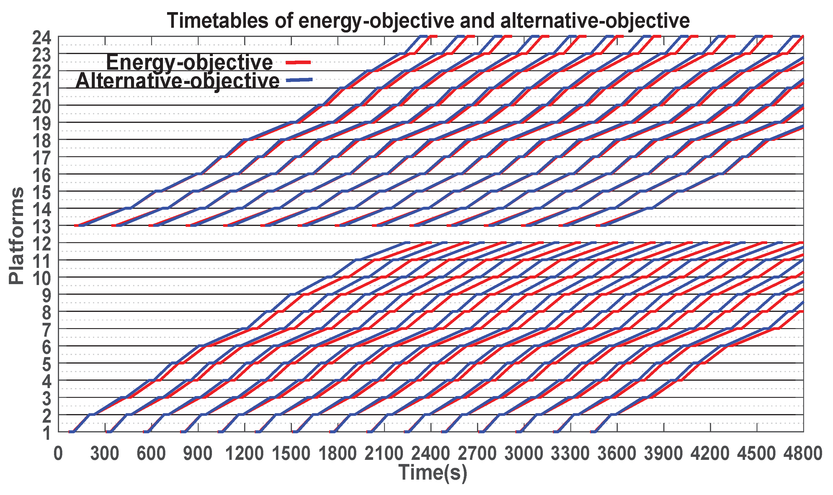
In this section, a timetable optimization model with a mixed-integer non-linear formulation is proposed to minimize the energy consumption in the planning horizon. The urban rail line is defined as a line network with a platform and track, which represent the node and link, respectively. The notations of the model are defined in the following.

3.1. Symbols

Parameters:

${\displaystyle N}$	number of stations,
${\displaystyle S}$	set of stations, S= {1, 2, ..., N},
${\displaystyle P}$	set of platforms, P = {1,2, ..., N, N + 1, ..., 2N},
${\displaystyle T}$	set of tracks, T = {1, 2, ..., N − 1, N + 1, ..., 2N − 1},
${\displaystyle s}$	index of station, $s\in S$,
${\displaystyle p}$	index of platform, $p\in P$,
${\displaystyle t}$	index of track, $t\in T$,
${\displaystyle l_t}$	length of track t,
${\displaystyle v_t^{min}}$	minimum average velocity in track t,
${\displaystyle v_t^{max}}$	maximum average velocity in track t,
${\displaystyle d{w}_{min}}$	minimum dwell time,
${\displaystyle d{w}_{max}}$	maximum dwell time,
${\displaystyle h_{min}}$	minimum headway,
${\displaystyle h_{max}}$	maximum headway,
${\displaystyle o{d}_{i,j}}$	origin-destination (o-d) demands from station i to station j,
${\displaystyle A_p}$	passenger volume that alights from platform p,
${\displaystyle B_p}$	passenger volume that boards at platform p,
Â${}_p$	average alighting rate at platform p,
B${}_p$	average boarding rate at platform p,
${\displaystyle Q_t}$	passenger volume in track t,
${\displaystyle Q_{max}}$	maximum passenger volume of the track in the line,
${\displaystyle a^{\left(r\right)}}$	alighting rate,
${\displaystyle b^{\left(r\right)}}$	boarding rate,
${\displaystyle Trai{n}_{cap}}$	train capacity,
${\displaystyle M^T}$	train mass,
${\displaystyle m_0}$	average passenger weight,
${\displaystyle F_{max}}$	maximum fleet size,
${\displaystyle TZ}$	turning back time at the depot or round-trip line.

Decision variables:

${\displaystyle a_p}$	arrival time of the first train at platform $p\in P$,
${\displaystyle d_p}$	departure time of the first train at platform $p\in P$,
${\displaystyle d{w}_p}$	dwell time of the first train at platform $p\in P$,
${\displaystyle T{B}_p}$	boarding time at platform $p\in P$,
${\displaystyle T{A}_p}$	alighting time at platform $p\in P$,
${\displaystyle L_t}$	average train passenger load in track t,
${\displaystyle M_t}$	total train load in track t,
${\displaystyle E_t}$	energy consumption in track t,
${\displaystyle R_t}$	running time in track t,
${\displaystyle v_t}$	average velocity in track t,
${\displaystyle f}$	frequency in the planning horizon,
${\displaystyle C}$	circle time,
${\displaystyle h}$	headway in the planning horizon.

3.2. Energy Consumption Function

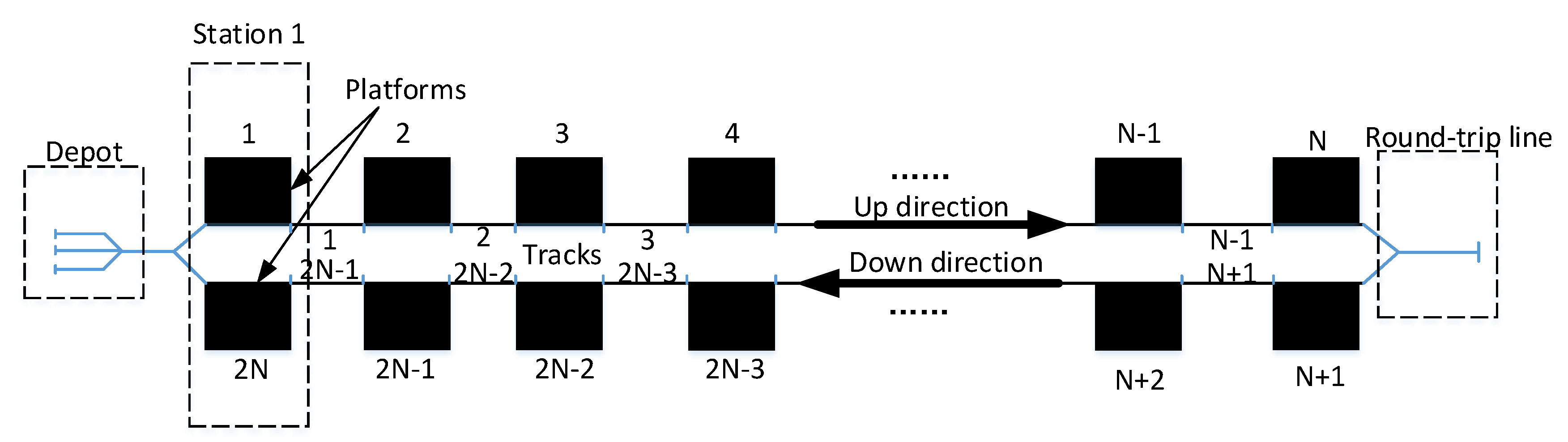
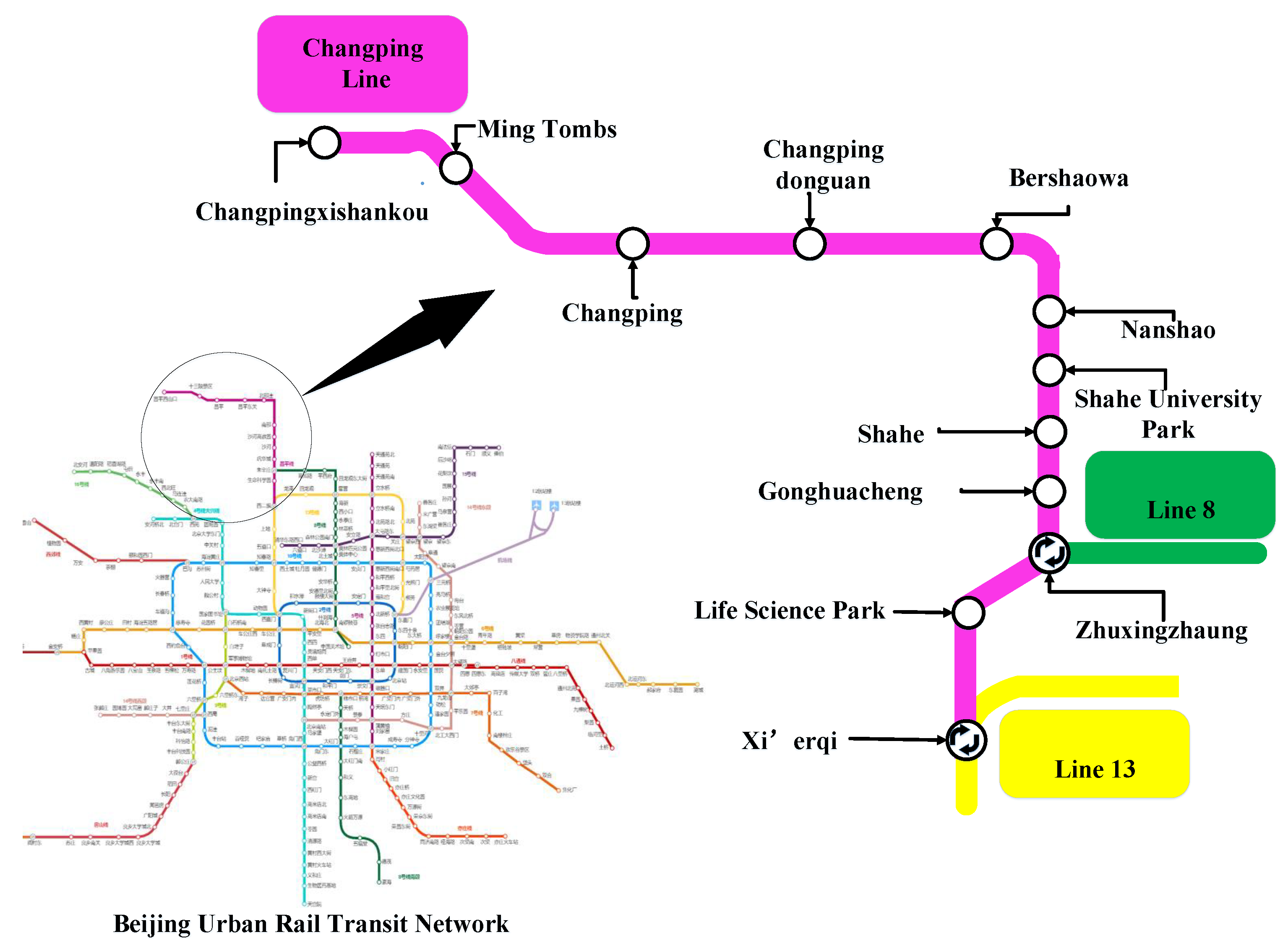
A bi-directional line network was taken into account. There are N stations and $2N$ platforms, as shown in Figure 2. Station set $S=\{1,2,...,N\}$, and platform set $P=\{1,2,...,N,N+1,...,2N\}$. For the sake of clarity, platforms $\{1,2...N\}$ are set in the upward direction, and platforms $\{N+1,...,2N\}$ are in the downward direction. Therefore, $2N-2$ links (tracks) $T=\{1,2,...,N-1,N+1,...,2N-1\}$ and two round-trip lines connect the $2N$ platforms. $\{1,2,...,N-1\}$ links (tracks) are in the upward direction, while $\{N+1,...,2N-1\}$ are also in the downward direction. In particular, N and $2N$ are excluded from set T, which actually correspond to the round-trips. Number N can be the round-trip line at the back of the station N, and number $2N$ can represent the round-trip to the depot before Station 1. We can see that if station $s\in S$, then $s\in P$ and $2N-s+1\in P$. 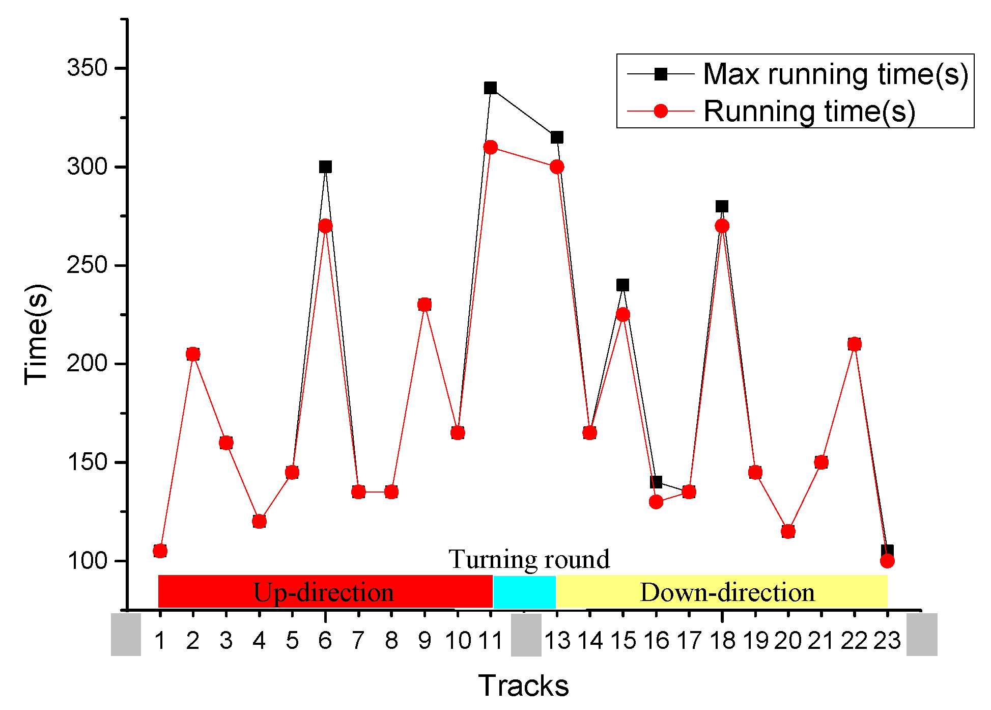For each track $t\in T$, there are some attributes: length of track $l_t$ and maximum and minimum average velocity $V_t^{max}$ and $V_t^{min}$ (for the technology requirement and safety considerations of the rail line).

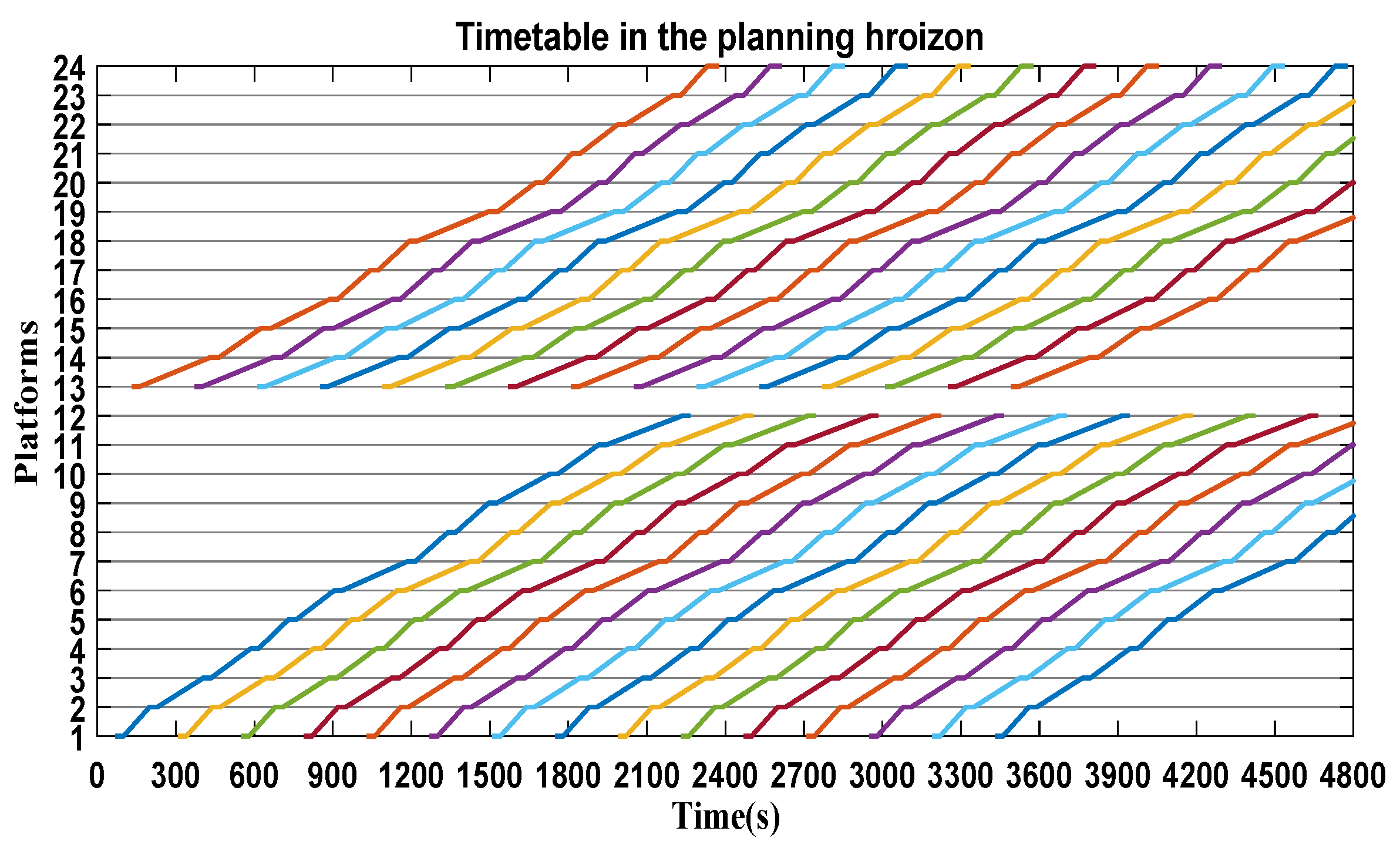
When the passenger demands and passenger-oriented objectives are considered to design a more energy-efficient timetable, both the departure and arrival time at each platform need to be determined. As the time is obtained, the trains will repeat the same running cycle with an interval of headway time (h), which is called the periodic timetable. The period usually lasts for 1–2 h. For instance, there is a cycle of 1 h in the evening peak from 17:30–18:30 in many metropolises. In the planning horizon, $a_p$ denotes the first arrival time at platform $p\in P$, while $d_p$ denotes the first departure time at platform $p\in P$, and $v_t$ represents the running speed at an average level on tracks $t\in T$. Therefore, the average running time of track t can be calculated using the formula $R_t=l_t/v_t$. To pursue the optimal energy consumption, once the average speed is given in each track, the train will be operated under the optimal profile, as mentioned in Howlett et al. (2009) [39], with the Pontryagin maximum principle.

There are several parts of energy consumption during the running process:

(1)

Energy consumption that comes from the running resistance $E_{rt}$.

(2)

Energy consumption that is from the air volume, which is absorbed by the train $E_{it}$.

(3)

Energy consumption that comes from the aerodynamic resistance $E_{at}$.

(4)

Energy consumption that offsets the kinetic energy, which is from the variation of the train on the tracks $E_{kt}$.

Then, we can calculate the total energy consumption in the track t as follows:

$$E_t=E_{kt}+(E_{rt}+E_{it}+E_{at})\times l_t$$

(1)

The total energy is a quadratic polynomial in $v_t$, which is an increasing function of the passenger load and speed. In this study, the total energy with various passenger loads is assumed to be a direct ratio to its growth. Furthermore, we can obtain the basic energy consumption of an empty train from the real recorded data. That is to say, if we get the passenger load and train mass, we can calculate the total energy.

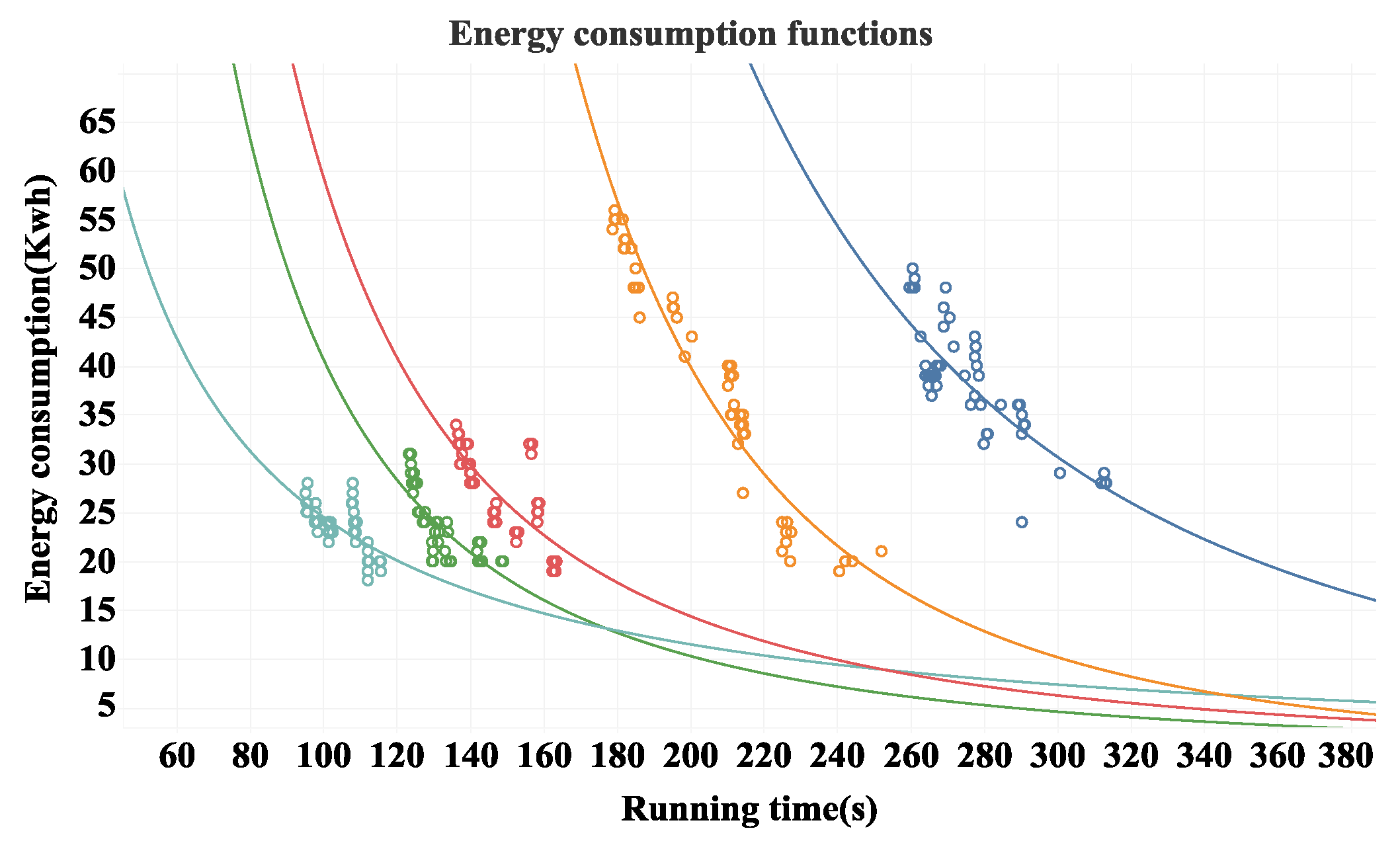
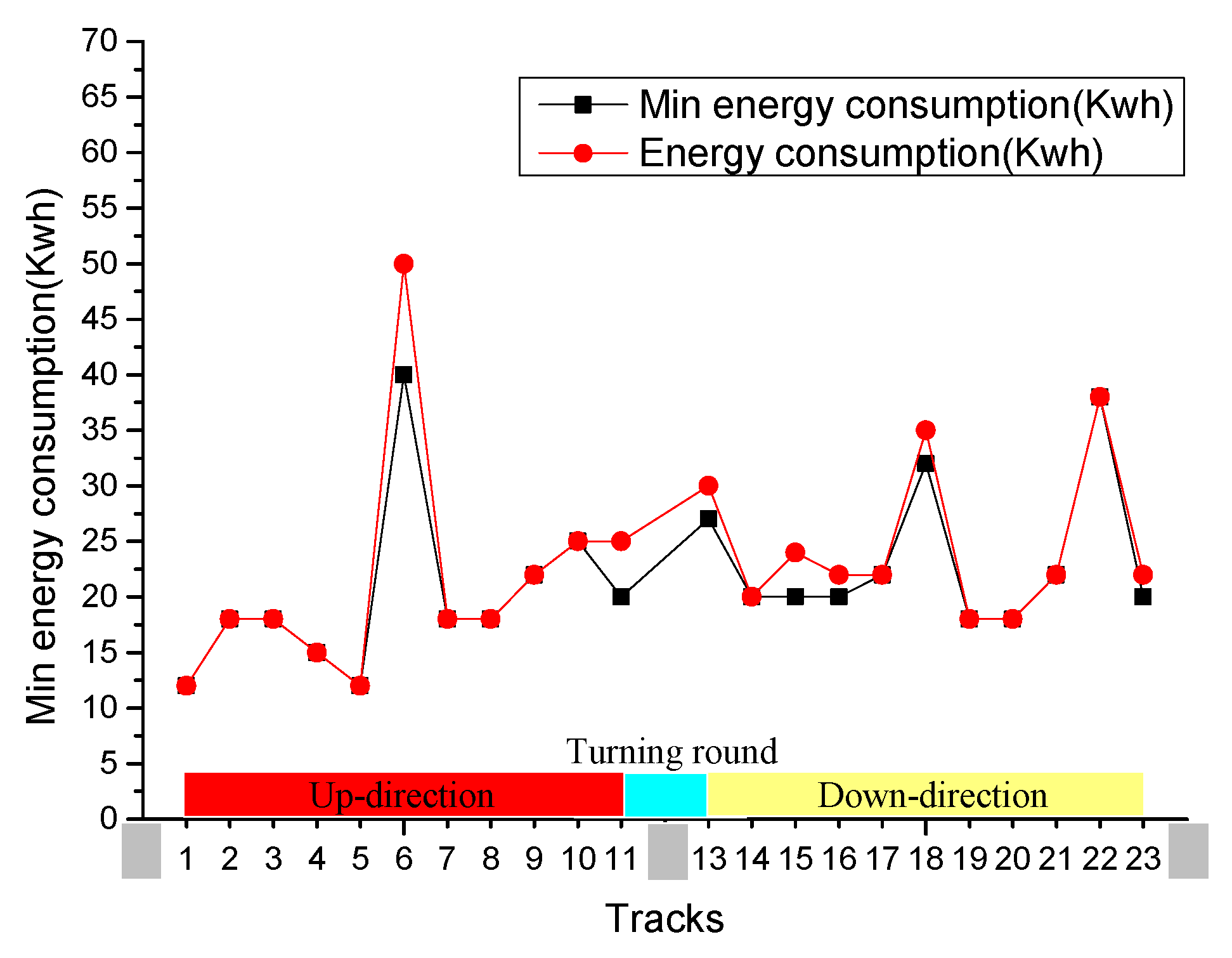
As shown in Figure 3, there are real-world statistics for different sections (different colors and trend lines represent the energy consumption in different sections). It is easy to observe that the most energy-efficient timetable will be obtained under the minimum average speed (maximum allowed running time). However, this is a single train condition with no constraints. If the headway and passenger accommodation constraints are taken into account, then it would be more complicated. The minimum average speed can always be invalidated because of the pressure from the operational efficiency.

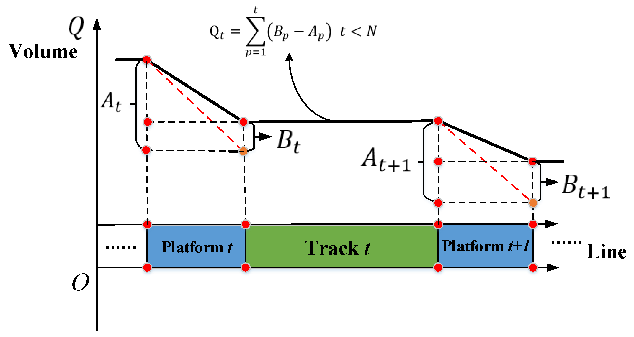
The energy consumed is a function of the average velocity (also the running time $R_t$) and train load $M_t$ (train mass $M^T$ and the total weight of passengers $L_t$ on the track t) in each track. Furthermore, the energy consumption in a cycle is the sum of each track $t\in T$ with the train running a whole circle on the bi-directional urban rail line. Therefore, it can be formulated as follows:

$$\sum _{t\in T}{E}_t(M_t,R_t)$$

(2)

Therefore, the total energy consumed during the planning horizon, E, including every train’s energy in the cycle, should be computed as follows:

$$E=f\times \sum _{t\in T}{E}_t(M_t,R_t)$$

(3)

We know that frequency f is associated with the train velocity since the faster a train runs, the higher the frequency is during the planning horizon, which also means higher energy consumption. However, if the frequency is too low, then the operational trains might fail to accommodate all passengers.

3.3. The Timetable Specification

OD: passenger demands in the form of the origin-destination (o-d) matrix:

$$o{d}_{i,j}\in OD;i,j\in S$$

There are two conditions. In the upward direction, $i<j$, $o{d}_{i,j}$ corresponds to the passenger volume from platforms i to j. Otherwise, for $i>j$, $o{d}_{i,j}$ is the passenger volume from platform $2N-i+1$ to $2N-j+1$.

Thus, in the planning horizon (1 h in this paper), the boarding and alighting passengers can be calculated as follows:

Firstly, the passengers boarding $B_p$ at platforms p can be computed as follows:

For platforms N and $2N$, there are no passengers boarding the train. Therefore:

$$B_p=\left\{\begin{array}{cc}{\displaystyle \sum _{j=p+1}^N}o{d}_{p,j},\hfill & \mathrm{if}p\in [1,N)\hfill \\ 0,\hfill & \mathrm{if}p=N\hfill \\ {\displaystyle \sum _{j=p+1}^{2N}}o{d}_{2N-p+1,2N-j+1},\hfill & \mathrm{if}p\in [N+1,2N)\hfill \\ 0,\hfill & p=2N\hfill \end{array}\right.$$

(4)

Similarly, the passengers alighting $A_p$ at platform p can be computed as follows:

For Platforms 1 and $N+1$, there are no passengers alighting from the train. Therefore:

$$A_p=\left\{\begin{array}{cc}0,\hfill & \mathrm{if}p=1\hfill \\ {\displaystyle \sum _{i=1}^{p-1}}o{d}_{i,p},\hfill & \mathrm{if}p\in (1,N]\hfill \\ 0,\hfill & \mathrm{if}p=N+1\hfill \\ {\displaystyle \sum _{i=N+1}^{p-1}}o{d}_{2N-i+1,2N-p+1},\hfill & \mathrm{if}p\in (N+1,2N]\hfill \end{array}\right.$$

(5)

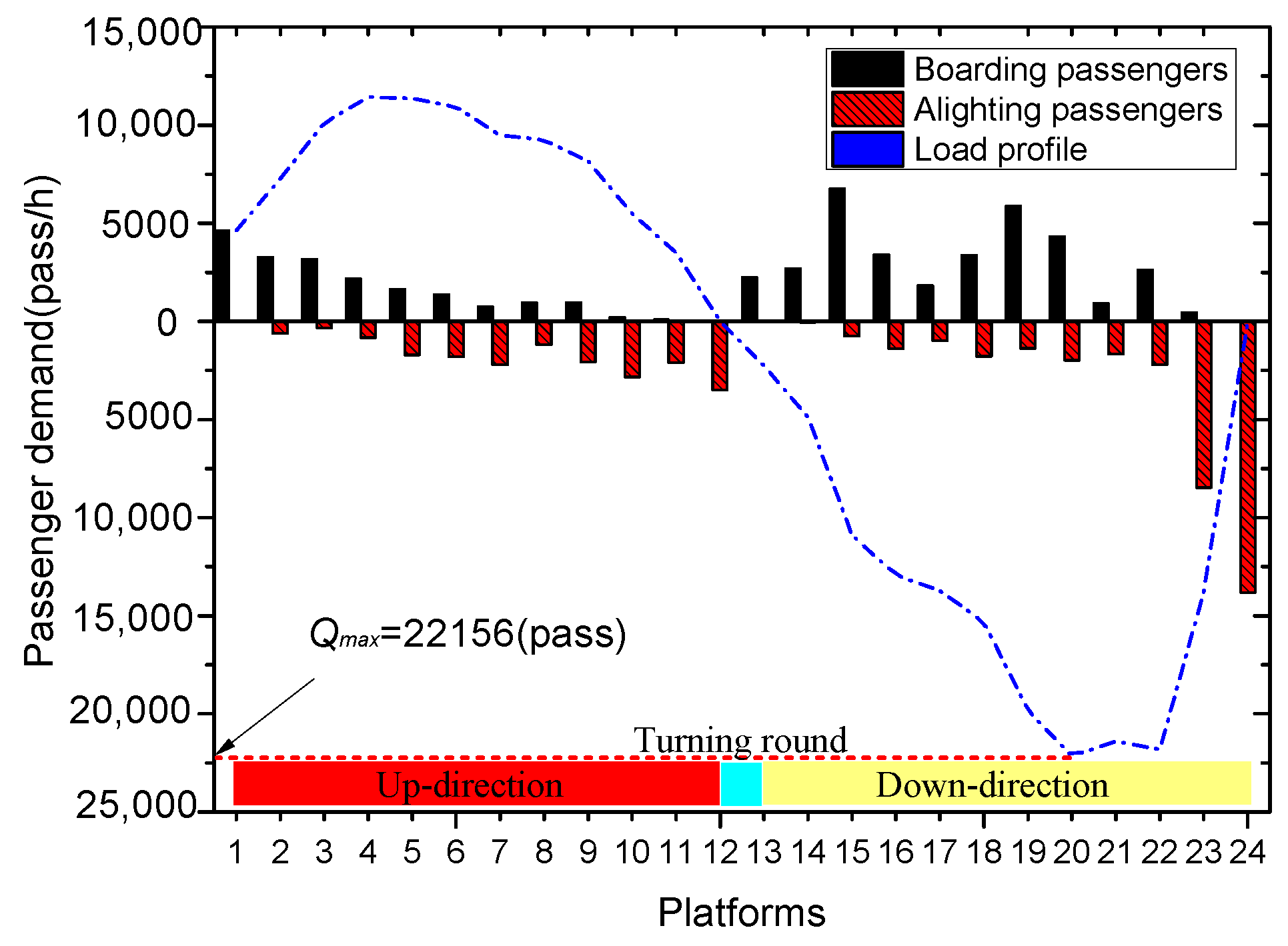
As for passenger volume in each track t, it can be computed through the accumulative process in linking platforms t to $t+1$. For instance, in the upward direction ($t<N$), as shown in Figure 4, the passenger volume in track t is ${\displaystyle \sum _{p=1}^t}(B_P-A_p)$.

Therefore, the passenger volumes in both directions are:

$$Q_t=\left\{\begin{array}{cc}{\displaystyle \sum _{p=1}^t}(B_p-A_p),\hfill & \mathrm{if}t\in [1,N)\hfill \\ {\displaystyle \sum _{p=N+1}^t}(B_p-A_p),\hfill & \mathrm{if}t\in [N+1,2N)\hfill \end{array}\right.$$

(6)

The largest passenger track can be found, and the maximum number of passengers in the tracks is:

$$Q_{max}=\underset{t\in T}{max}{Q}_t$$

(7)

$Q_{max}$ is an essential parameter for accommodating the passenger demand. Furthermore, it is a constraint on transport capacity.

Assuming that the passengers arrive uniformly, the average passengers boarding and alighting the trains are applied in the model. A planning horizon of 1 h (3600 s) was taken into account in this study. Average boarding and alighting rates are (measured as passengers per second):

$${\widehat{B}}_p=\frac{B_p}{3600},{\widehat{A}}_p=\frac{A_p}{3600}$$

(8)

The running time on track t begins at the departure time at platform t and ends at the arrival time at platform $t+1$. Therefore:

$$R_t=a_{t+1}-d_t$$

(9)

Furthermore, there are always velocity limitations in the running sections for safety and geographical reasons. Therefore, there are bounded constraints on the running time of sections:

$$\frac{l_t}{V_{max}}\le R_t\le \frac{l_t}{V_{min}}$$

(10)

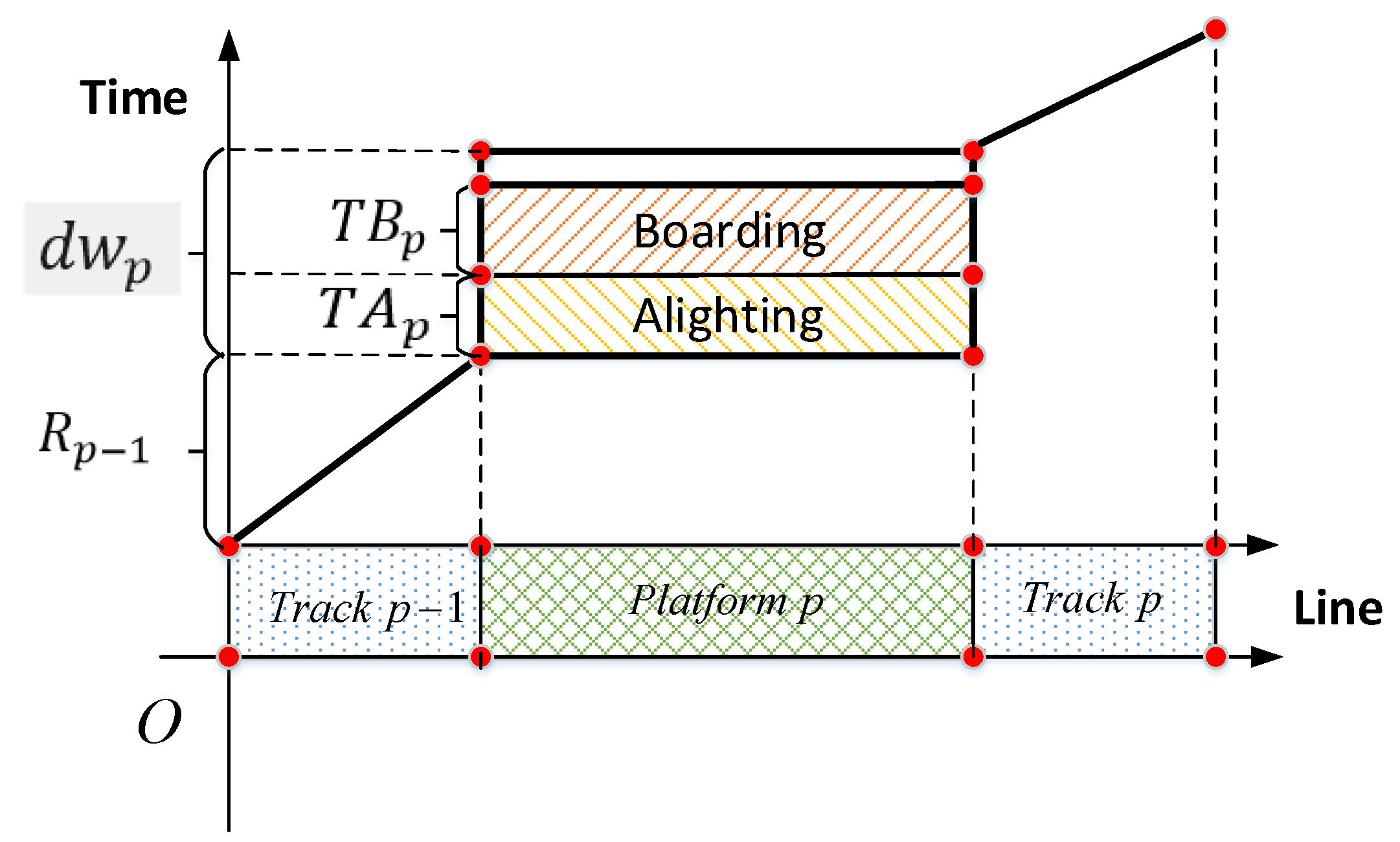
Similarly, the dwell time, $d{w}_p$, begins at the arrival time at platform p and ends at the departure time of platform p. Therefore:

$$d{w}_p=d_p-a_p$$

(11)

In addition, there are constraints on the boarding and alighting of passengers during the dwelling process. Furthermore, $a^{\left(r\right)}$ denotes the empirical alighting, while $b^{\left(r\right)}$ denotes the boarding rates. Both are measured as seconds per passenger, which are determined by the width and number of train doors. Furthermore, the alighting time $TA$ and boarding time $TB$ at platform p can be computed as follows:

$$T{A}_p={\widehat{A}}_p\times h\times a^{\left(r\right)}$$

(12)

$$T{B}_p={\widehat{B}}_p\times h\times b^{\left(r\right)}$$

(13)

The dwell time must be long enough to complete the alighting and boarding processes (as shown in Figure 5). Therefore, the dwell time should cover the alighting time and boarding time: $d{w}_p\ge (T{A}_p+T{B}_P)$, which are arranged as:

$$d{w}_p\ge h\times (a^{\left(r\right)}\times {\widehat{A}}_p+b^{\left(r\right)}\times {\widehat{B}}_p)$$

(14)

There are always bounded values for headway. On the one hand, the minimum headway is determined by the signaling system and safety considerations. On the other hand, the maximum value is usually restricted to the service level or government tasks. Therefore:

$$h_{min}\le h\le h_{max}$$

(15)

The departure frequency f, which represents the train quantity in the line during the planning horizon, is associated with the headway by:

$$3600=f\times h$$

(16)

To ensure the frequency is an integer, h must be a divisor of 3600. In this case, as in Canca et al. (2016) [4], there are alternative headway values, for instance 120, 180, 240, 300, 360, 600, 720, 900, 1200, and 1800 s.

To avoid train pileups, the dwell time at each platform cannot be greater than the headway:

$$d{w}_p\le h$$

(17)

Furthermore, to maintain the order of the passengers on the platforms for safety purposes, there is bounded dwell time:

$$d{w}_{min}\le d{w}_p\le d{w}_{max}$$

(18)

The cycle time C, which is the time consumed by a train in running a loop in the bi-directional line, can be computed as:

$$C=2\times TZ+\sum _{t\in T}{R}_t+\sum _{p\in p}d{w}_p$$

(19)

where $TZ$ denotes the turning back time. There is always a technical standard for the turn back time under the turn back facilities and signal system. Furthermore, the headway is associated with the fleet size F, which is a relationship in:

$$F=C/h$$

(20)

Then, by replacing the headway h with $f/3600$, the fleet size can be calculated as:

$$F=C\times f/3600$$

(21)

We can see that if cycle time $C\ge 3600$ s, then $F\ge f$. If cycle time $C<3600$ s (there may be short lines for a short cycle), then $F<f$.

The train quantity is also limited by consideration of the fixed investment. Therefore, the fleet size cannot be greater than the maximum train quantity:

$$F\le F_{max}$$

(22)

For a fixed train unit, there is a corresponding capacity $Trai{n}_{cap}$ due to the consideration of the limited room and passenger comfort. To guarantee that all passenger demands (all $OD$ demands) are satisfied with the maximum capacity, frequency f should satisfy the constraint as follows:

$$Q_{max}\le Trai{n}_{cap}\times f$$

(23)

The constraints (23) can be another form by replacing the f by relation $f\times h=3600$, then:

$$Q_{max}\times h\le Trai{n}_{cap}\times 3600$$

(24)

Therefore, if the train capacity is fixed after determining the train units, then the carrying quantity in one hour is $Trai{n}_{cap}/h_{min}$. Additionally, with the increase in $Q_{max}$, the headway should be shorter.

Finally, if the average passenger weight is $m_0$, the average train passenger load $L_t$ on track t for a train in the planning horizon can be calculated as:

$$L_t=\frac{Q_t\times m_0}{f}=\frac{Q_t\times m_0\times h}{3600}$$

(25)

3.4. First MINLP Formulation

Therefore, the model is a Mixed Integer Non-Linear (MINLP) problem. Moreover, non-linearities include the objective function E and the constraints (†) and (‡). Since we are in pursuit of the exact solution and a global optimum, we will linearize them in the following section.

$$MinE=Min\{f\times \sum _{t\in T}{E}_t(M_t,R_t)\},$$

(26)

$$\begin{array}{c}{R}_t=a_{t+1}-d_t,\\ \frac{l_t}{V_{max}}\le R_t\le \frac{l_t}{V_{min}},\\ d{w}_p=d_p-a_p,\end{array}$$

$$\begin{array}{c}d{w}_p\le h,\\ d{w}_{min}\le d{w}_p\le d{w}_{max},\\ d{w}_p\ge h\times (a^{\left(r\right)}\times {\widehat{A}}_p+b^{\left(r\right)}\times {\widehat{B}}_p),\\ L_t=\frac{Q_t\times m_0\times h}{3600},\\ C=2\times TZ+{\displaystyle \sum _{t\in T}}{R}_t+{\displaystyle \sum _{p\in P}}d{w}_p,\\ h_{min}\le h\le h_{max},\\ f\times h=3600,(†)\\ F=C/h,(‡)\\ F\le F_{max},\\ Q_{max}\times h\le Trai{n}_{cap}\times 3600,\\ R_t,L_t,a_p,d{w}_p,d_p\ge 0,\\ C,F,h\ge 0,andintegers,\forall t\in T,\forall p\in P,\end{array}$$

4. The Timetable Optimization Model: Mixed Integer Linear Programming Formulation

To find the exact solutions more easily, we linearize the objective function and non-linear constraints in this section and develop a timetable optimization model with a mixed-integer linear programming formulation. The linearizing process is concluded in the following.

4.1. Linearizing the Objective Function

In real operations, the profiles in a section are not arbitrary, but a set of alternative train speed profiles. There are different operation levels g, which correspond to different running times $R_g$. When the profile level is changed, the running time and energy consumption will be changed. The basic energy consumption of an empty train on track t at level g is $E_{t,g}^0$. For the sake of clarity, as shown in Figure 6, there are three levels to the operational process in the section, which is from Ming Tomb to Changpingxishankou of the Changping Line in Beijing urban rail transit. Thus, there are three profiles with three different running times and corresponding energy consumption. When the passengers are loaded on the train, then the total weight is $M^T+L_t$. Thus, the energy can be approximately equal to $(1+\frac{L_t}{M^T})E_{t,g}^0$.

Consider that there is a set of operation levels on track t, $G_t$. Introduce a set of binary variables ${\theta }_{g,t}$. If the level g is selected, then the ${\theta }_{g,t}=1$; else ${\theta }_{g,t}=0$. For a running section, there is only one level g that can be selected; therefore:

$$\sum _g^{G_t}{\theta }_{g,t}=1$$

(27)

$$R_t=\sum _g^{G_t}{\theta }_{g,t}\times R_{g,t}$$

(28)

Therefore, the energy consumption $E_t(R_t,L_t)$ can be replaced by:

$$\sum _g^{G_t}{\theta }_{g,t}(1+\frac{L_t}{M^T})E_{t,g}^0$$

(29)

Define a new set of variables ${\rho }_{g,t}$ so that ${\rho }_{g,t}=(1+\frac{L_t}{M^T})$ if ${\theta }_{g,t}=1$. Then, a set of constraints should be introduced:

$$(1+\frac{L_t}{M^T})-\Lambda (1-{\theta }_{g,t})\le {\rho }_{g,t}\le (1+\frac{L_t}{M^T})+\Lambda (1-{\theta }_{g,t}),\forall t\in T,g\in G_t$$

(30)

$${\rho }_{g,t}\le {\theta }_{g,t}\Lambda ,\forall t\in T,g\in G_t$$

(31)

$${\rho }_{g,t}\ge 0,\forall t\in T,g\in G_t$$

(32)

where $\Lambda$ is the upper bound; for instance, $(1+\frac{L_{max}}{M^T})E_{max}^0$.

Therefore, the objective function $E_t(R_t,L_t)$ can be replaced by:

$$\sum _g^{G_t}{\rho }_{g,t}\times E_{t,g}^0$$

(33)

Set H includes the possible headway values. To ensure the integer values of f in 3600 s, the alternative headway in H can be:

$$H=\{120,180,240,300,360,600,720,900,1800\}$$

Furthermore, the corresponding frequency set is:

$$\Omega =\{30,20,15,12,10,6,5,4,3,2\}$$

Then, $h_m(m=1,2...,|H\left|\right)$ denotes the alternative elements of H. $f_m(m=1,2...,|\Omega \left|\right)$ denotes the alternative elements of $\Omega$. To make sure $h_m\times f_m=3600$, $h_m$ is in ascending order, while $f_m$ is in descending order.

We introduced a series of binary variables ${\delta }_m(m=1,2...,|\Omega \left|\right)$. Since the passenger demand is strong in the peak hour, $\Omega =\{30,20,15,12,10,6\}$ and $H=\{120,180,240,300,360,600\}$ are in our consideration. The binary variables ${\delta }_m$ and the elements $h_m$ can be utilized to represent the headway as the sum of their product as follows:

$$h=\sum _{m=1}^{|\Omega |}{\delta }_m\times h_m$$

(34)

Similarly, the frequency can be expressed as:

$$f=\sum _{m=1}^{|\Omega |}{\delta }_m\times f_m$$

(35)

Therefore, the sum of the binary variables ${\delta }_m$ should be equal to one:

$$\sum _{m=1}^{|\Omega |}{\delta }_m=1$$

(36)

By replacing with the new variables, the objective can be expressed in the following formation:

$$\begin{array}{c}\hfill Min\sum _{m=1}^{|\Omega |}{\delta }_m\times f_m\sum _{t\in T}\sum _g^{G_t}{\rho }_{g,t}\times E_{t,g}^0\\ \hfill =\sum _{m=1}^{|\Omega |}\sum _{t\in T}\sum _g^{G_t}{\rho }_{g,t}\times E_{t,g}^0\times {\delta }_m\times f_m\\ \hfill =\sum _{t\in T}\sum _g^{G_t}\sum _{m=1}^{|\Omega |}({\rho }_{g,t}\times {\delta }_m)\times (E_{t,g}^0\times f_m)\end{array}$$

(37)

In the above formulas, replace $({\rho }_{g,t}\times {\delta }_m)$ with the new variable ${\lambda }_{g,t,m}$, which must take the value ${\rho }_{g,t}$ while ${\delta }_m=1$. This can be achieved through sets of constraints:

$${\rho }_{g,t}-\Delta (1-{\delta }_m)\le {\lambda }_{g,t,m}\le {\rho }_{g,t}+\Delta (1-{\delta }_m),\forall t\in T,g\in G_t,m=1,...,|\Omega |$$

(38)

$${\lambda }_{g,t,m}\le {\delta }_m\Delta ,\forall t\in T,g\in G_t,m=1,...,|\Omega |$$

(39)

$${\lambda }_{g,t,m}\ge 0,\forall t\in T,g\in G_t,m=1,...,|\Omega |$$

(40)

where $\Delta$ is the upper bound; for instance, $(1+\frac{L_{max}}{M^T})E_{max}^0{f}_{max}$.

Finally, the linear formulation of the objective is shown as follows:

$$Min\sum _{t\in T}\sum _g^{G_t}\sum _{m=1}^{|\Omega |}{\lambda }_{g,t,m}(E_{t,g}^0\times f_m)$$

(41)

4.2. Linearizing the Non-Linear Constraints

The constraints † and ‡) are non-linear. After introducing the binary variables ${\delta }_m$ and sets of H and $\Omega$ above, the constraint † is linearized. Then, the constraint ‡ can be rewritten in:

$$C=\sum _{m=1}^{|\Omega |}{\delta }_m\times h_m\times F$$

(42)

Then, a set of variables ${\alpha }_m$ is introduced. If ${\delta }_m=1$, then ${\alpha }_m=F$. Therefore, it can be achieved by sets of constraints:

$$F-\Psi (1-{\delta }_m)\le {\alpha }_m\le F+\Psi (1-{\delta }_m),\forall m=1,...,|\Omega |$$

(43)

$${\alpha }_m\le {\delta }_m\Psi ,\forall m=1,...,|\Omega |$$

(44)

$${\alpha }_m\ge 0,\forall m=1,...,|\Omega |$$

(45)

where $\Psi$ is the upper bound; for example, $\Psi =F_{max}\times h_{max}$. Then, the constraints ‡ can be rewritten as follows:

$$C=\sum _{m=1}^{|\Omega |}{\alpha }_m\times h_m$$

(46)

4.3. The MILP Timetable Optimization Model

With the objective and constraints linearized, the MINLP model can be converted into an MILP formulation as follows:

$$Min\sum _{t\in T}\sum _g^{G_t}\sum _{m=1}^{|\Omega |}{\lambda }_{g,t,m}(E_{t,g}^0\times f_m),$$

$$\begin{array}{c}(1+\frac{L_t}{M^T})-\Lambda (1-{\theta }_{g,t})\le {\rho }_{g,t}\le (1+\frac{L_t}{M^T})+\Lambda (1-{\theta }_{g,t}),\\ {\rho }_{g,t}\le {\theta }_{g,t}\Lambda ,\\ {\rho }_{g,t}\ge 0,\\ {\rho }_{g,t}-\Delta (1-{\delta }_m)\le {\lambda }_{g,t,m}\le {\rho }_{g,t}+\Delta (1-{\delta }_m),\\ {\lambda }_{g,t,m}\le {\delta }_m\Delta ,\\ {\lambda }_{g,t,m}\ge 0,\\ F-\Psi (1-{\delta }_m)\le {\alpha }_m\le F+\Psi (1-{\delta }_m),\\ {\alpha }_m\le {\delta }_m\Psi ,\\ {\alpha }_m\ge 0,\end{array}$$

$$\begin{array}{c}{R}_t={\displaystyle \sum _g^{g_t}}{\theta }_{g,t}\times R_{g,t},{\displaystyle \sum _g^{G_t}}{\theta }_{g,t}=1,\\ h={\displaystyle \sum _{m=1}^{|\Omega |}}{\delta }_m\times h_m,f={\displaystyle \sum _{m=1}^{|\Omega |}}{\delta }_m\times f_m,\\ {\displaystyle \sum _{m=1}^{|\Omega |}}{\delta }_m=1,{\displaystyle \sum _{m=1}^{|\Omega |}}{\alpha }_m\times h_m=C,\\ h_{min}\le h\le h_{max},\\ R_t=a_{t+1}-d_t,\\ \frac{l_t}{V_{max}}\le R_t\le \frac{l_t}{V_{min}},\\ d{w}_p=d_p-a_p,\\ d{w}_p\le h,\\ d{w}_{min}\le d{w}_p\le d{w}_{max},\\ d{w}_p\ge h\times (a^{\left(r\right)}\times {\widehat{A}}_p+b^{\left(r\right)}\times {\widehat{B}}_p),\\ L_t=\frac{Q_t*m_0\times h}{3600},\\ C={\displaystyle \sum _{t\in T}}{R}_t+{\displaystyle \sum _{p\in P}}d{w}_p+2\times TZ,\\ C={\displaystyle \sum _{m=1}^{|\Omega |}}{\alpha }_m\times h_m\\ Q_{max}\times h\le Trai{n}_{cap}\times 3600,\\ F\le F_{max},\\ R_t,L_t,a_p,d{w}_p,d_p\ge 0,\\ C,F,h\ge 0,integers,\\ {\delta }_m,{\theta }_{g,t}=\{0,1\},\\ \forall p\in P,t\in T,g\in G_t,m=1,...,|\Omega |.\end{array}$$

The complexity of the model is analyzed. The continuous variables and their numbers are: $L_t\left(\right|T\left|\right),R_t\left(\right|T\left|\right),a_p\left(\right|P\left|\right),$$d{w}_p\left(\right|P\left|\right),d_p\left(\right|P\left|\right),{\rho }_{g,t}\left(\right|G\left|\right|T\left|\right),{\lambda }_{g,t,m}\left(\right|G\left|\right|T\left|\right|\Omega \left|\right)$. The integer variables and their numbers are: $F\left(\right|1\left|\right),C\left(\right|1\left|\right),h\left(\right|1\left|\right),$$f\left(\right|1\left|\right)$. The binary variables and their numbers are: ${\delta }_m|\Omega |,$${\theta }_{g,t}\left(\right|G\left|\right|T\left|\right)$. The total number of constraints is: $9+4\left|T\right|+3\left(\right|P|+|G|+|\Omega |+|G\left|\right|T|+|G\left|\right|T\left|\right|\Omega \left|\right)$.

5. An Alternative Objective Function from the Perspective of System Cost

The aim of designing a timetable is optimizing energy consumption, which is pretty significant for environmental protection. However, it seems not profitable for urban rail system operators. The reason is that there are other costs like driver salaries, train unit acquirement, maintenance cost, etc., during the operations. Among these costs, two main ones come from the personnel expenses and those generated from train unit acquisition. Therefore, to minimize the total cost from an operational system, we employed an alternative objective function, which takes into consideration the train unit and operation cost. There are three types of value coefficients as follows:

$C_e$: The average electricity price of 1 kWh.

$C_a$: The hourly cost, which comes from train unit acquisition and maintenance during the operations.

$C_s$: The average hourly salary corresponding to the driver. Therefore, the alternative objective function can be:

$$Min{C}_e\left(\sum _{t\in T}\sum _g^{G_t}\sum _{m=1}^{|\Omega |}{\lambda }_{g,t,m}(E_{t,g}^0\times f_m)\right)+(C_a+C_s)F$$

(47)

We can see that the first term of the sum is the energy cost, and the latter corresponds to the cost of investments in the train unit and personnel.

6. A Case Study: Based on the Beijing Changping Line

To give a detailed illustration of the proposed model, we considered the bi-directional line (Changping Line) of Beijing urban rail transit. The operational section of Changping Line is a two-way line running from the Xi’erqi station to the Changpingxishankou station, with operational mileage of 31.9 km and a total of 12 stations opened (as illustrated in Figure 7). Since the Changping Line is located in the suburbs of Beijing, it is not overcrowded in the peak hours. Information about the stations, the length of open tracks, ranges of the dwell time, and profile attributes are given in

Table 1. Basic line and profile attributes of the Beijing Changping Line.

Station Index & Segment	Length (m)	Maximum Dwell Time (s)	Minimum Dwell Time (s)	Running Time Options (s)	Energy (kWh)
1 Changpingxishankou-MingTombs	1213.13	60	30	95, 100, 105	21, 15, 12
2 MingTombs-Changping	2811.86	60	30	175, 190, 205	35, 24, 18
3 Changping-Changpingxishankou	2433	60	30	140, 150, 160	36, 27, 18
4 Changpingxishankou-Beishaowa	1683	60	30	110, 115, 120	25, 18, 15
5 Beishaowa-Nanshao	1958.96	60	30	135, 140, 145	25, 20, 12
6 Nanshao-Shahe university Park	5357.04	60	30	250, 270, 300	65, 50, 40
7 Shahe university Park-Shahe	1964.7	60	30	125, 130, 135	25, 21, 18
8 Shahe-Gonghuacheng	2025.17	60	30	125, 130, 135	27, 22, 18
9 Gonghuacheng-Zhuxinzhaung	3799.83	60	30	205, 220, 230	30, 26, 22
10 Zhuxinzhuang-Life Science Park	2367.97	60	30	150, 155, 165	40, 32, 25
11 Life Science Park-Xierqi	5440.94	60	30	290, 310, 340	45, 25, 20
Turnaround	-	-	-	-	-
13 Xierqi-Life Science Park	5440.94	60	30	270, 300, 315	45, 30, 27
14 Life Science Park-Zhuxinzhuang	2367.97	60	30	155, 160, 165	32, 24, 20
15 Zhuxinzhuang-Gonghuacheng	3799.83	60	30	210, 225, 240	40, 24, 20
16 Gonghuacheng-Shahe	2025.17	60	30	125, 130, 140	25, 22, 20
17 Shahe-Shahe university Park	1964.7	60	30	120, 130, 135	32, 25, 22
18 Shahe university Park-Nanshao	5357.04	60	30	260, 270, 280	49, 35, 32
19 Nanshao-Beishaowa	1958.96	60	30	135, 140, 145	32, 26, 18
20 Beishaowa-Changpingdongguan	1683	60	30	105, 110, 115	30, 21, 18
21 Changpingdongguan-Changping	2433	60	30	135, 145, 150	35, 25, 22
22 Changping-Ming Tombs	2811.86	60	30	180, 200, 210	55, 42, 38
23 Ming Tombs-Changpingxishankou	11,213.13	60	30	95, 100, 105	27, 22, 20
Depot	-	-	-	-	-

. The profile energy consumption was derived from the real experiment data of the empty train. The dwell time limits were in consideration of the passenger waiting time and maintaining platform order.

The operational parameters are listed in

Table 2. Parameter settings in the numerical experiments.

Parameters	Symbol	Value
Maximum train quantity	$F_{max}$	22
Train mass (t)	$M^T$	205
Train capacity (pass)	$Trai{n}_{cap}$	1760
Average passenger weight (kg)	$m_0$	65
Alighting rate (s/pass)	$a^{\left(r\right)}$	0.05
Boarding rate (s/pass)	$b^{\left(r\right)}$	0.08
Turning back time (s)	TZ	300
Electricity price (RMB/kWh)	$C_e$	0.7
Acquisition cost coefficients (RMB/h)	$C_a$	2000
Driver salaries (RMB/h)	$C_s$	80
Maximum speed (km/h)	$V_{max}$	100
Minimum speed (km/h)	$V_{min}$	40

. There are 22 trains belonging to the operation branch of Changping line. The net weight of each train is about 205 ton, while the train seating capacity is1460 people. The peak hour coefficient is about 1.2 based on a survey of the actual ride. Therefore, the train capacity is 1.2 * 1460 = 1760 people. The average passenger weight is given as 65 kg. The alighting and boarding rates are empirical, which refer to Canca et al. (2017). The turning back time for the Beijing urban rail transit networks is a technical standard that should be no more than 5min. The cost coefficients are obtained from the operations department.

Table 3. OD-passenger matrix during the peak hour 7:00–8:00 of the Changping line.

O\D	1	2	3	4	5	6	7	8	9	10	11	12
1	0	619	275	374	571	209	578	590	257	481	209	454
2	452	0	61	47	355	578	688	61	234	333	306	608
3	1684	934	0	423	333	128	364	49	454	522	382	511
4	382	288	247	0	443	227	61	261	295	337	171	371
5	2427	1512	196	124	0	657	247	38	148	216	49	292
6	3007	2279	265	247	86	0	275	175	178	295	38	405
7	1189	1120	405	326	275	61	0	20	257	265	162	61
8	376	275	86	178	491	257	158	0	247	257	117	344
9	890	461	148	326	608	124	738	121	0	128	553	275
10	3106	1278	326	124	178	553	178	511	502	0	99	99
11	82	216	257	220	185	209	355	209	392	560	0	78
12	170	99	275	121	158	175	355	151	502	185	56	0

shows the passenger matrix for the peak hour of the planning horizon 7:00–8:00, which was extracted from the AFC (Automatic Fare Collection) data of Changping Line. The passenger demand (boarding and alighting numbers) and load profile at each station are shown in Figure 8. We can see that the maximum section volume ($Q_{max}$) was from Beishaowa-Changpingdongguan, with about 22,156 passengers. We can see that there was a slight imbalance in passenger demands between the two directions, which was a result of more passengers commuting from a residential zone to work places or schools.

Case 1: The objective function includes minimizing the energy consumption only. We obtained the minimum energy consumption (9413.3 kWh) and timetable under all constraints. To show the energy savings, we calculated the maximum energy consumption (14,458.5 kWh, which was under the fastest profile. Therefore, 14,458.5 − 9413.3 = 5045.2 kWh were saved, which accounts for about a 35% reduction. The results of arrival time, departure time, and dwell time of the first train in the planning horizon $[0,3600]$ s are listed in

Table 4. Timetable under an energy consumption objective.

Platforms\Time	Arrive Time (s)	Dwell Time (s)	Departure Time (s)
1	70	30	100
2	200	30	230
3	405	30	435
4	585	30	615
5	730	30	760
6	905	30	935
7	1185	30	1215
8	1340	30	1370
9	1495	30	1525
10	1730	30	1760
11	1915	30	1945
12	2235	30	2265
13	131.1	30	161.1
14	431.1	33.8	465
15	625	38.5	663.5
16	888.5	30	918.5
17	1043.5	30	1073.5
18	1193.5	30	1223.5
19	1493.5	36	1529.5
20	1674.5	30	1704.5
21	1814.5	30	1844.5
22	1989.5	30	2019.5
23	2199.5	30	2230.1
24	2330.1	46	2376.1

. We can see that the dwell time was relatively even, except for three platforms, which is in accordance with the passenger flow. Therefore, in most of the stations, the passenger flow was not overly crowded. For clarity, all departures in both directions are shown in Figure 9. It illustrates that the distributions of the departure time in the up and down direction was symmetrical. Furthermore, the arrival time in the up direction was earlier than that in the down direction, which may be caused by the imbalance in passenger demands between the two directions; because the passenger flow in the up direction was higher than that in the down direction.

The running time and energy consumption of each track are shown in Figure 10 and Figure 11. Compared with the max running time of each track, the actual running time was equal to those of most tracks. Correspondingly, the actual energy consumption levels were equal to the minimum of most tracks, which conforms to the pursuit of minimum energy consumption.

Furthermore, we calculated the travel time of the whole odpairs as shown in Figure 12. There were two surfaces of the up and down direction. The surfaces were relatively smooth, which indicates that the running time and departure time were well distributed. From the intersection angles with their horizontal plane, we can see that the travel time in up direction (from Station 1–12) increased slightly more quickly than in the down direction (from Station 12–1). Overall, the distributions of travel time were balanced in the whole line.

Case 2: From the perspective of system cost, we can obtain the minimum system cost for the operational process. As listed in

Table 5. Result parameters with two different objectives.

Objectives\Items	Total Cost (RMB)	Total Energy (kWh)	f	h (s)	F	C (s)
Energy objective	52,349.3	9413.3	15	240	22	5280
Alternative objective	52,202.5	12,175	15	240	21	5040

, to pursue the goal of energy conservation only, the energy consumption (9413.3 kWh) can be reduced by one-third compared with the system cost viewpoint (12,175 kWh). However, the fleet size of the energy objective was one more than the alternative objective, which means an increase in driver and acquisition cost: 80 + 2000 = 2080 (RMB). Moreover, the cycle time also raised 5280 − 5040 = 240 (s).

The driver and train were cycled slowly. Overall, the total cost of the energy objective was 52,349.3 (RMB), very nearly equal to that of the alternative objective, 52,202.5 (RMB). The cost savings was 6.6% compared with the maximum system cost 55,880.9 (RMB). The frequency and headway were the same. Therefore, there was little difference in the waiting time of the passenger.

Running time and energy consumption with two different objectives are given in

Table 6. Running time and energy consumption with two different objectives.

Items	Running Time (s)		Energy Consumption (kWh)
Tracks\Obj	Energy Objective	Alternative Objective	Energy Objective	Alternative Objective
1	105	100	12	15
2	205	175	18	35
3	160	150	18	27
4	120	115	15	18
5	145	145	12	12
6	270	250	50	65
7	135	125	18	25
8	135	125	18	27
9	230	205	22	30
10	165	155	25	32
11	310	290	25	45
13	300	270	30	45
14	165	160	20	24
15	225	225	24	24
16	130	125	22	25
17	135	120	22	32
18	270	270	35	35
19	145	145	18	18
20	115	110	18	21
21	150	145	22	25
22	210	180	38	55
23	100	100	22	22

. Thus, we see that the running time under the alternative objective in each track tended to be shorter than that under the energy objective. Therefore, from the viewpoint of the system cost, the train tended to run faster and made full use of the train fleet size. For clarity, as shown in Figure 13 and Figure 14, compared with the maximum time and minimum energy consumption level, the actual running time under the alternative objective deviated from the maximum time, which shows high efficiency in the operation. In summary, the results of the alternative objective were a compromise between the maximum energy consumption and energy objective.

As shown in Figure 15, the departure time of the train under the alternative objective was earlier. In addition, the high operational efficiency may cause extra energy consumption, but a reduction in total cost. Therefore, there is a trade-off between energy conservation and operational efficiency. The solutions under the balanced condition between energy conservation and operational efficiency were found by the model. Furthermore, whether the view was oriented toward energy conservation or system cost, the departure times in the up and down directions were in equilibrium.

7. Conclusions

Urban inhabitants relying too much on urban rail transit due to its advantages of safety, punctuality, high energy, and large capacity, there has been a quick rise in energy consumption. For the sake of pursuing cost savings and environmental protection, there is an urgent demand for energy conservation.

To address the problem of increasing energy consumption in the urban rail transit system, we aimed to design an energy-efficient timetable in this paper. First, we proposed a timetable optimization model in the mixed-integer non-linear formulation. Then, the objective and constraints were linearized. The mixed-integer linear programming model was employed, which could be solved by the commercial solver Gurobi. Moreover, from the perspective of system cost, we presented an alternative objective. To validate the model, real data from the Changping Line of Beijing urban rail transit were applied as a case study. Subsequently, the results showed that the designed timetable could achieve about a 35% energy reduction compared with the maximum energy consumption and 6.6% cost savings compared with the maximum system cost. We find that there was a trade-off between operational efficiency and energy consumption. The energy objective was prone to lower energy consumption, while the alternative objective tended toward high operational efficiency with fast running time. Furthermore, the direction with higher passenger flow also tended to run faster.

The modeling framework still had some limitations. For instance, the passenger flow was roughly considered. A dynamic passenger flow will be more practical. In summary, there are several future research directions. We could consider passenger behavior and passenger costs, such as the travel times of passengers. There is feedback about passenger flow after a timetable change. Therefore, a dynamic equilibrium between the timetable and passengers should be found. Moreover, the regenerative energy produced during the braking process could be utilized in the same substation, which could reduce both the energy and total costs, so it should be modeled. Finally, there is not always a single line, but an urban rail transit network in a city. The energy conservation should be extended to the urban rail transit networks for the entire operational system. There are several future research directions. Finally, a scientific algorithm should be proposed when this problem is for a large-scale condition.

References

1. Gonzlez-Gil, A.; Palacin, R.; Batty, P.; Powell, J. A systems approach to reduce urban rail energy consumption. Energy Convers. Manag. 2014, 80, 509–524. [Google Scholar] [CrossRef] [Green Version]
2. Huang, Y.; Yu, H.; Yin, J.; Hu, H.; Bai, S.; Meng, X.; Wang, M. An integrated approach for the energy-efficient driving strategy optimization of multiple trains by considering regenerative braking. Comput. Ind. Eng. 2018, 126, 399–400. [Google Scholar] [CrossRef]
3. Scheepmaker, G.M.; Goverde, R.M.P.; Kroon, L.G. Review of energy-efficient train control and timetabling. Oper. Res. 2017, 257, 355–376. [Google Scholar] [CrossRef]
4. Canca, D.; Barrena, E.; De-Los-Santos, A.; Andrade-Pineda, J.L. Setting lines frequency and capacity in dense railway rapid transit networks with simultaneous passenger assignment. Transp. Res. Part B Methodol. 2016, 93, 251–267. [Google Scholar] [CrossRef]
5. Peter, P.; Howlett, P. Optimal driving strategies for a train journey with speed limits. Anziam. J. 1994, 36, 38–49. [Google Scholar] [Green Version]
6. Yang, X.; Li, X.; Ning, B.; Tang, T. A survey on energy-efficient train operation for urban rail transit. IEEE Trans. Intell. Transp. Syst. 2016, 17, 2–13. [Google Scholar] [CrossRef]
7. Huang, K.; Wu, J.; Yang, X.; Gao, Z.; Liu, F.; Zhu, Y. Discrete train speed profile optimization for urban rail transit: A data-driven model and integrated algorithms based on machine learning. J. Adv. Transp. 2019, 2019. [Google Scholar] [CrossRef]
8. Yang, X.; Li, X.; Gao, Z.; Wang, H.; Tang, T. A cooperative scheduling model for timetable optimization in subway systems. IEEE Trans. Intell. Transp. Syst. 2013, 14, 438–447. [Google Scholar] [CrossRef]
9. Albrecht, A.; Howlett, P.; Vu, X.; Pudney, P.; Zhou, P. The key principles of optimal train control-part 1: Formulation of the model, strategies of optimal type, evolutionary lines, location of optimal switching points. Transp. Res. Part B Methodol. 2016, 94, 482–508. [Google Scholar] [CrossRef]
10. Albrecht, A.; Howlett, P.; Vu, X.; Pudney, P.; Zhou, P. The key principles of optimal train control-part 2: Existence of an optimal strategy, the local energy minimization principle, uniqueness, computational techniques. Transp. Res. Part B Methodol. 2016, 94, 509–538. [Google Scholar] [CrossRef]
11. Ye, H.; Liu, R. A multiphase optimal control method for multi-train control and scheduling on railway lines. Transp. Res. Part B Methodol. 2016, 93, 377–393. [Google Scholar] [CrossRef] [Green Version]
12. Howlett, P.G.; Cheng, J. Optimal driving strategies for a train on a track with continuously varying gradient. Aust. Math. Soc. 1997, 38, 388–410. [Google Scholar] [CrossRef] [Green Version]
13. Khmelnitsky, E. On an optimal control problem of train operation. IEEE Trans. Autom. Control 2000, 45, 1257–1266. [Google Scholar] [CrossRef]
14. Albrecht, A.R.; Howlett, P.G.; Pudney, P.J.; Vu, X. Energy-efficient train control: From local convexity to global optimization and uniqueness. Automatica 2013, 49, 3072–3078. [Google Scholar] [CrossRef]
15. Rodrigo, E.; Tapia, S.; Mera, J.M.; Soler, M. Optimizing electric rail energy consumption using the lagrange multiplier technique. J. Transp. Eng. 2013, 139, 321–329. [Google Scholar] [CrossRef]
16. Wang, P.; Goverde, R.M.P. Multiple-phase train trajectory optimization with signalling and operational constraints. Transp. Res. Part C Emerg. Technol. 2016, 69, 255–275. [Google Scholar] [CrossRef]
17. Wang, P.; Goverde, R.M.P. Multi-train trajectory optimization for energy efficiency and delay recovery on single-track railway lines. Transp. Res. Part B Methodol. 2017, 105, 340–361. [Google Scholar] [CrossRef]
18. Shakibayifar, M.; Hassannayebi, E.; Jafary, H.; Sajedinejad, A. Stochastic optimization of an urban rail timetable under time-dependent and uncertain demand. Appl. Stoch. Models Bus. Ind. 2017, 33, 640–661. [Google Scholar] [CrossRef]
19. Wang, L.; Yang, L.; Gao, Z.; Huang, Y. Robust train speed trajectory optimization: A stochastic constrained shortest path approach. Front. Eng. Manag. 2017, 4, 408–417. [Google Scholar] [CrossRef]
20. Gainanov, D.N.; Nenad, M.; Rasskazova, V.A. Maximum independent set in planning freight railway transportation. Front. Eng. Manag. 2018, 5, 499–506. [Google Scholar]
21. Hassannayebi, E.; Zegordi, S.H.; Amin-Naseri, M.R.; Yaghini, M. Optimizing headways for urban rail transit services using adaptive particle swarm algorithms. Public Transp. 2018, 10, 23–62. [Google Scholar] [CrossRef]
22. Hu, S.; Liu, C. Optimizing headways for mass rapid transit services. Transp. Eng. 2014, 140, 1943–5436. [Google Scholar] [CrossRef]
23. Kang, L.; Wu, J.; Sun, H.; Zhu, X.; Gao, Z. A case study on the coordination of last trains for the beijing subway network. Transp. Res. Part B Methodol. 2015, 72, 112–127. [Google Scholar] [CrossRef]
24. Hassannayebi, E.; Zegordi, S.H.; Yaghini, M. Train timetabling for an urban rail transit line using a lagrangian relaxation approach. Appl. Math. Model. 2016, 40, 9892–9913. [Google Scholar] [CrossRef]
25. Huo, J.; Wu, J.; Kang, L.; Wang, B. Railway timetable rescheduling based on priority and train order entropy. Comput. Civ. Eng. 2016, 30, 04016006. [Google Scholar] [CrossRef]
26. Guo, X.; Sun, H.; Wu, J.; Jin, J.; Zhou, J.; Gao, Z. Multiperiod-based timetable optimization for metro transit networks. Transp. Res. Part B Methodol. 2017, 96, 46–67. [Google Scholar] [CrossRef]
27. Canca, D.; Zarzo, A. Design of energy-efficient timetables in two-way railway rapid transit lines. Transp. Res. Part B Methodol. 2017, 102, 142–161. [Google Scholar] [CrossRef]
28. Sparing, D.; Goverde, R.M.P. A cycle time optimization model for generating stable periodic railway timetables. Transp. Res. Part B Methodol. 2017, 98, 198–223. [Google Scholar] [CrossRef]
29. Zhou, L.; Tong, L.; Chen, J.; Tang, J.; Zhou, X. Joint optimization of high-speed train timetables and speed profiles: A unified modeling approach using space-time-speed grid networks. Transp. Res. Part B Methodol. 2017, 97, 157–181. [Google Scholar] [CrossRef] [Green Version]
30. Yin, J.; Wang, Y.; Tang, T.; Xun, J.; Su, S. Metro train rescheduling by adding backup trains under disrupted scenarios. Front. Eng. Manag. 2017, 4, 418–427. [Google Scholar] [CrossRef] [Green Version]
31. Wang, P.; Goverde, R.M.P. Multi-train trajectory optimization for energy-efficient timetabling. Eur. J. Oper. Res. 2019, 272, 621–635. [Google Scholar] [CrossRef]
32. Gao, Z.; Yang, L. Energy-saving operation approaches for urban rail transit systems. Front. Eng. Manag. 2019, 6, 139–151. [Google Scholar] [Green Version]
33. Chevrier, R.; Pellegrini, P.; Rodriguez, J. Energy saving in railway timetabling: A bi-objective evolutionary approach for computing alternative running times. Transp. Res. Part C Emerg. Technol. 2013, 37, 20–41. [Google Scholar] [CrossRef] [Green Version]
34. Li, X.; Lo, H.K. Energy minimization in dynamic train scheduling and control for metro rail operations. Transp. Res. Part B Methodol. 2014, 70, 269–284. [Google Scholar] [CrossRef]
35. Yang, S.; Wu, J.; Yang, X.; Sun, H.; Gao, Z. Energy-efficient timetable and speed profile optimization with multi-phase speed limits: Theoretical analysis and application. Appl. Math. Model. 2018, 56, 32–50. [Google Scholar] [CrossRef]
36. Sun, H.; Wu, J.; Ma, H.; Yang, X.; Gao, Z. A bi-objective timetable optimization model for urban rail transit based on the time-dependent passenger volume. IEEE Trans. Intell. Transp. Syst. 2019, 20, 604–615. [Google Scholar] [CrossRef]
37. Yang, S.; Wu, J.; Yang, X.; Liao, F.; Li, D.; Wei, Y. Analysis of energy consumption reduction in metro system using rolling stop-skipping patterns. Comput. Ind. Eng. 2019, 127, 129–142. [Google Scholar] [CrossRef]
38. Yang, X.; Chen, A.; Wu, J.; Gao, Z.; Tang, T. An energy-efficient rescheduling approach under delay perturbations for metro systems. Transp. B. Transp. Dyn. 2019, 7, 386–400. [Google Scholar] [CrossRef]
39. Howlett, P.G.; Pudney, P.; Vu, X. Local energy minimization in optimal train control. Automatica 2009, 45, 2692–2698. [Google Scholar] [CrossRef]
Figure 1. Energy consumption during 2010–2017 in Beijing urban rail transit.
Energies 12 02686 g001
Figure 2. Line network.
Energies 12 02686 g002
Figure 3. Energy consumption functions.
Energies 12 02686 g003
Figure 4. Passenger volume in each track t.
Energies 12 02686 g004
Figure 5. Alighting and boarding constraints of dwell time.
Energies 12 02686 g005
Figure 6. Different profiles with different levels.
Energies 12 02686 g006
Figure 7. Changping Line of the Beijing urban rail transit network.
Energies 12 02686 g007
Figure 8. Passenger demand and load profile of each platform during 7:00–8:00.
Energies 12 02686 g008
Figure 9. Timetable under an energy consumption objective.
Energies 12 02686 g009
Figure 10. Running time of each track under an energy consumption objective.
Energies 12 02686 g010
Figure 11. Energy consumption of each track under an energy consumption objective.
Energies 12 02686 g011
Figure 12. Travel time of od pairs under an energy consumption objective.
Energies 12 02686 g012
Figure 13. Running time with two different objectives.
Energies 12 02686 g013
Figure 14. Energy consumption with two different objectives.
Energies 12 02686 g014
Figure 15. Timetables with two different objectives.
Energies 12 02686 g015