A Simple and Robust Shock-Capturing Approach for Discontinuous Galerkin Discretizations

Abstract
1. Introduction
2. Governing Equations and Numerical Discretization
2.1. Governing Equations
2.2. Discontinuous Galerkin Discretization
2.3. Space-Time Discretization: ADER-DG
2.3.1. The Local Space-Time DG Predictor
2.3.2. The Corrector Step
3. Shock-Capturing in the Discontinuous Galerkin Method
3.1. Shock Detector
- Calculate from ,
- March solution forward one time-step and calculate a candidate solution ,
- Calculate from ,
- If , an element is not considered to be a troubled element. Otherwise, the current element might be a troubled element. Here, is a threshold value that depends on the polynomial order of the element.
- For elements with , calculate . If , then the current element is a troubled element. Here, is an empirically determined value.
3.2. Filtering
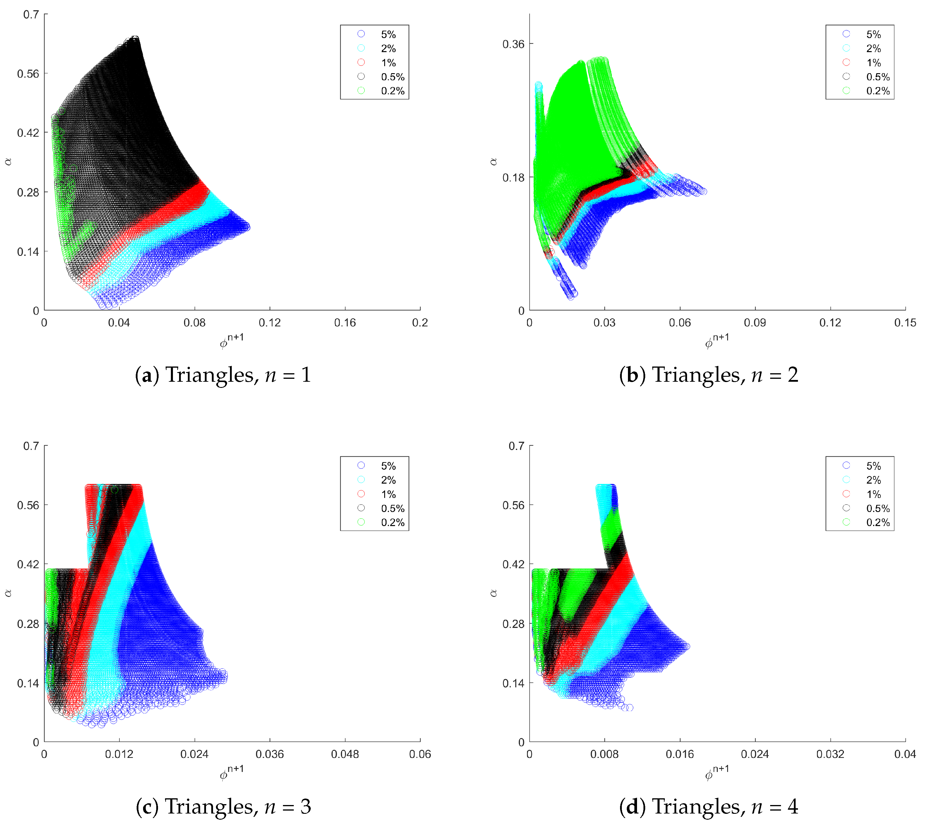
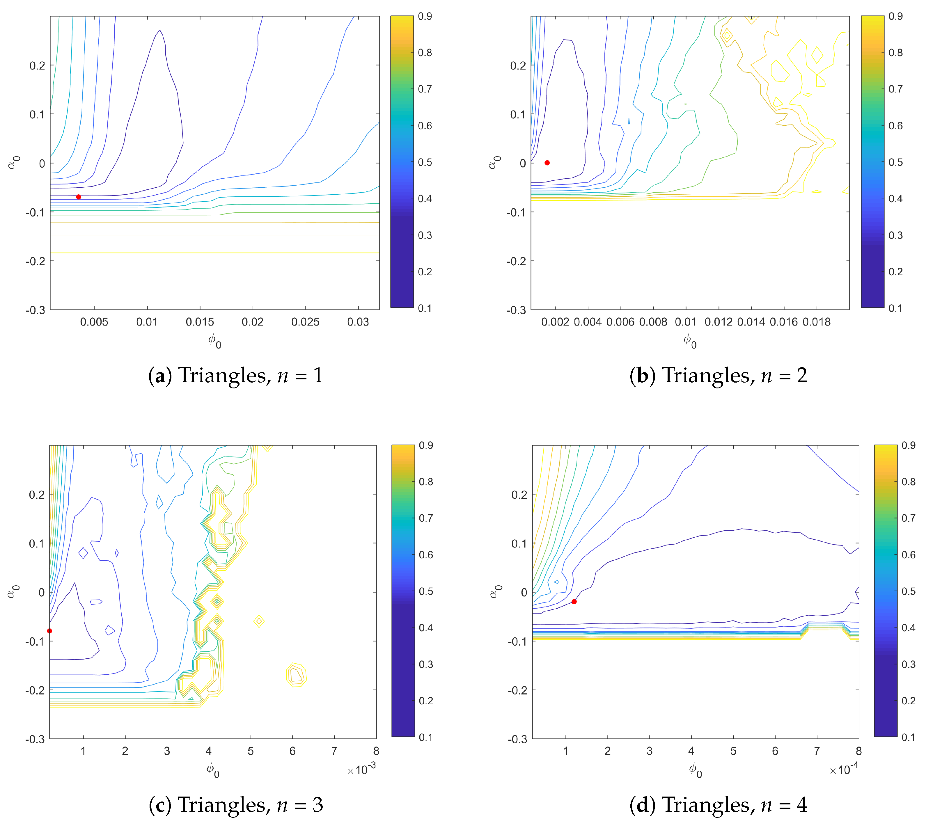
3.3. Correlation between and
4. Numerical Simulation Results
4.1. Isentropic Vortex Problem
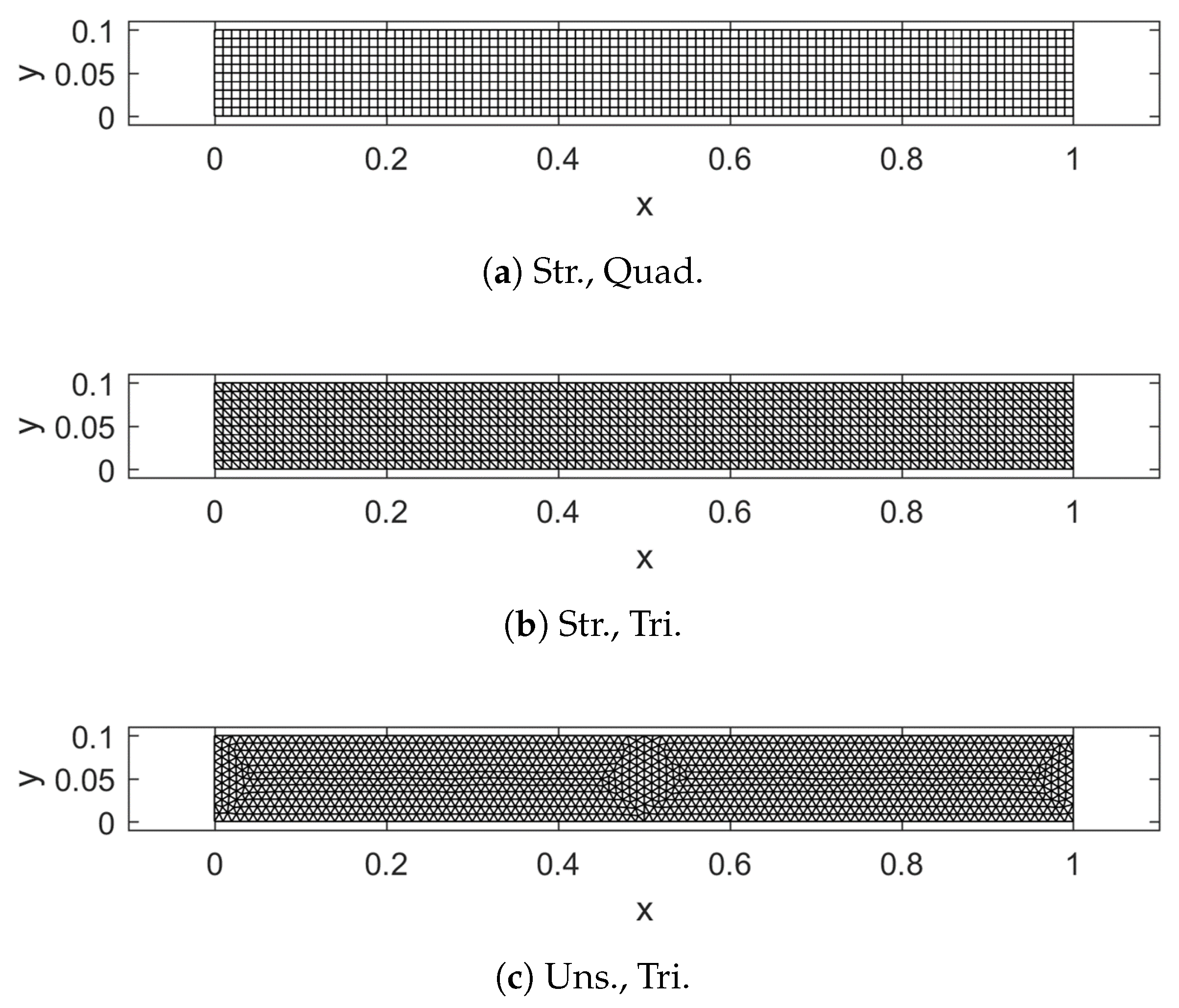
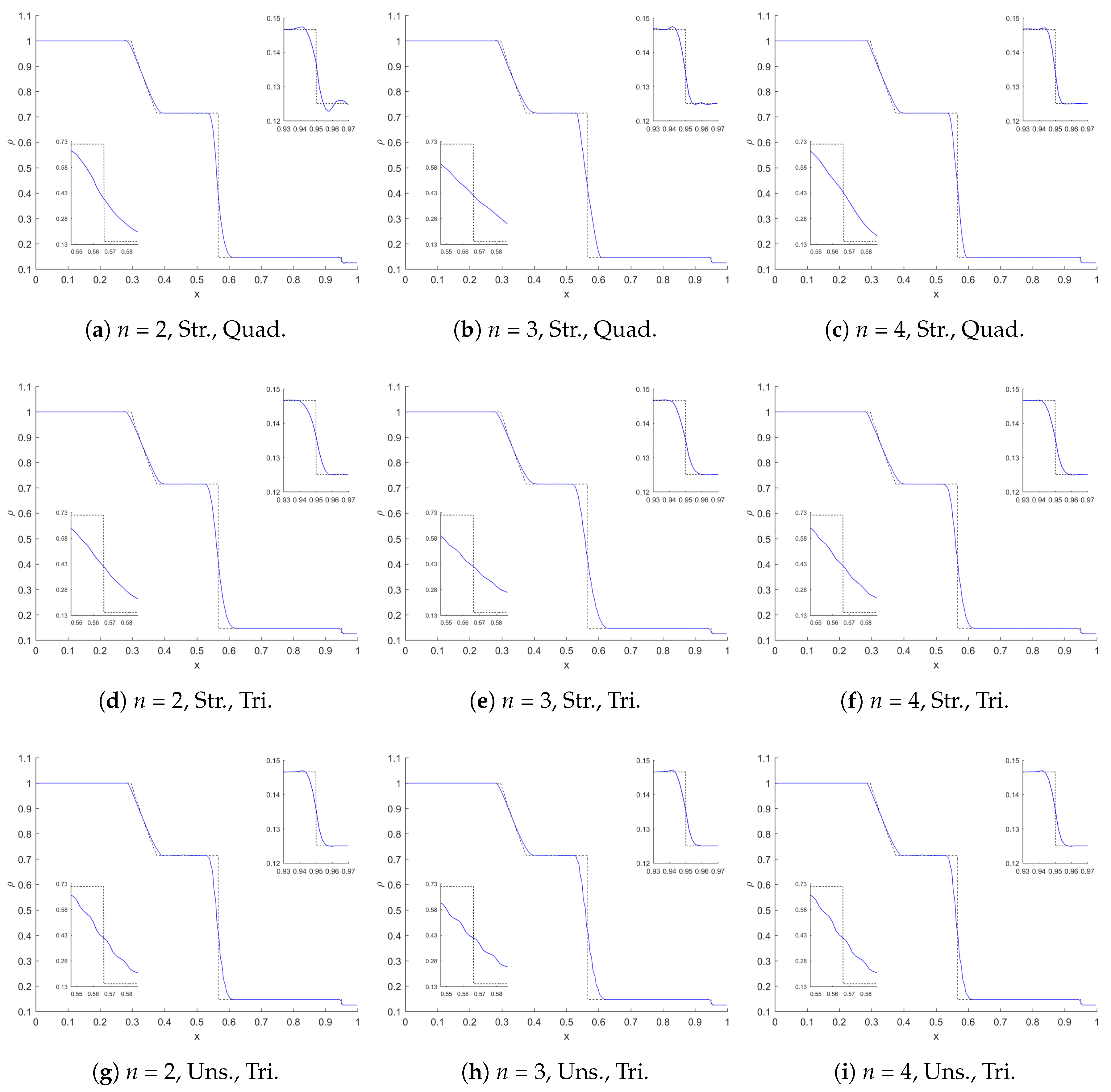
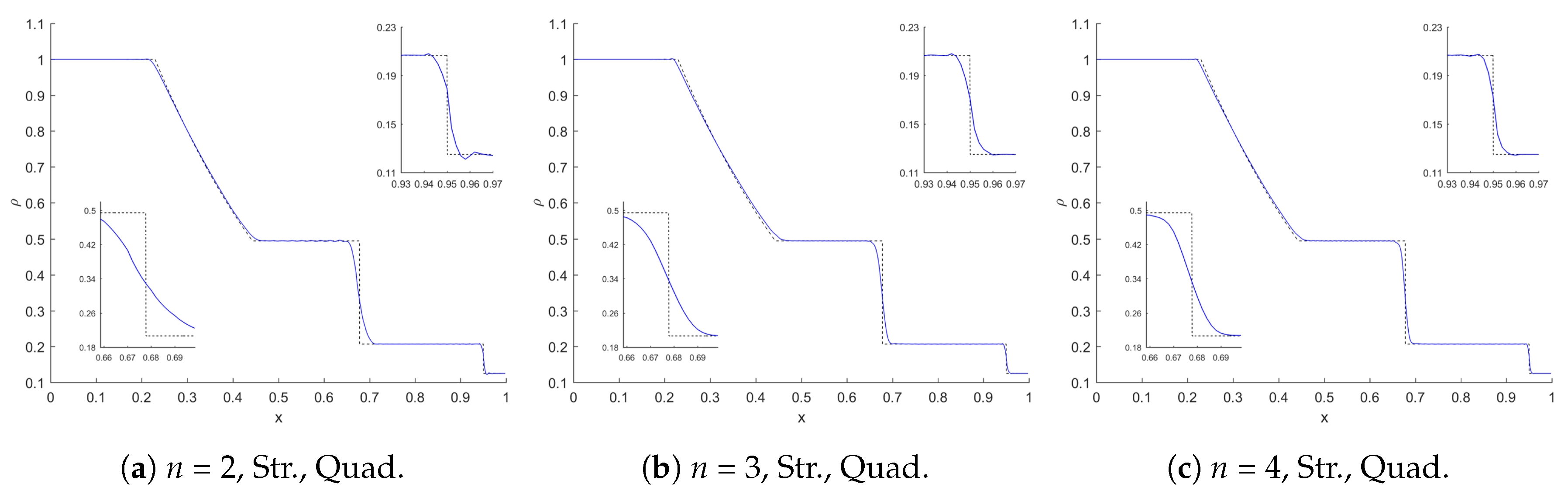
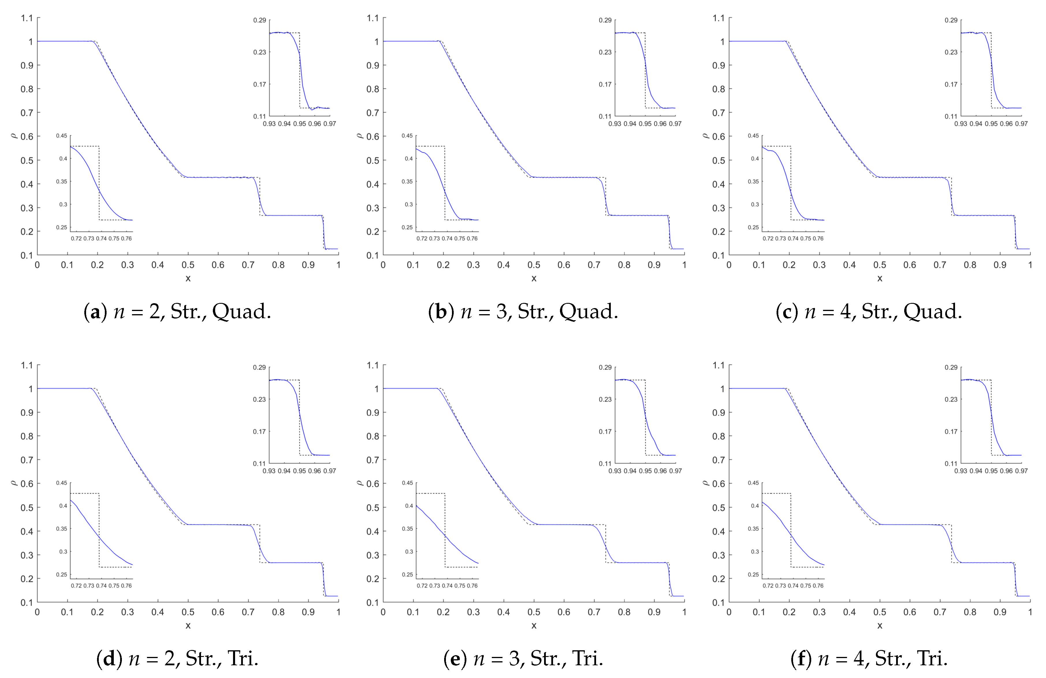
4.2. Shock Tube Problem
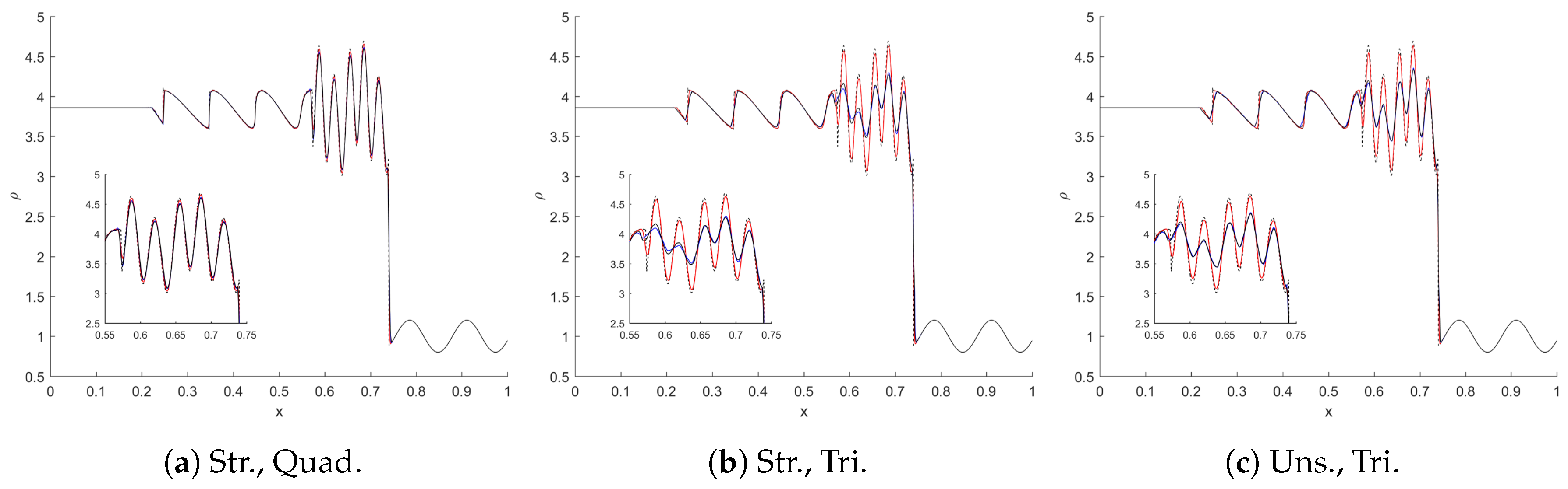
4.3. Shu–Osher Problem
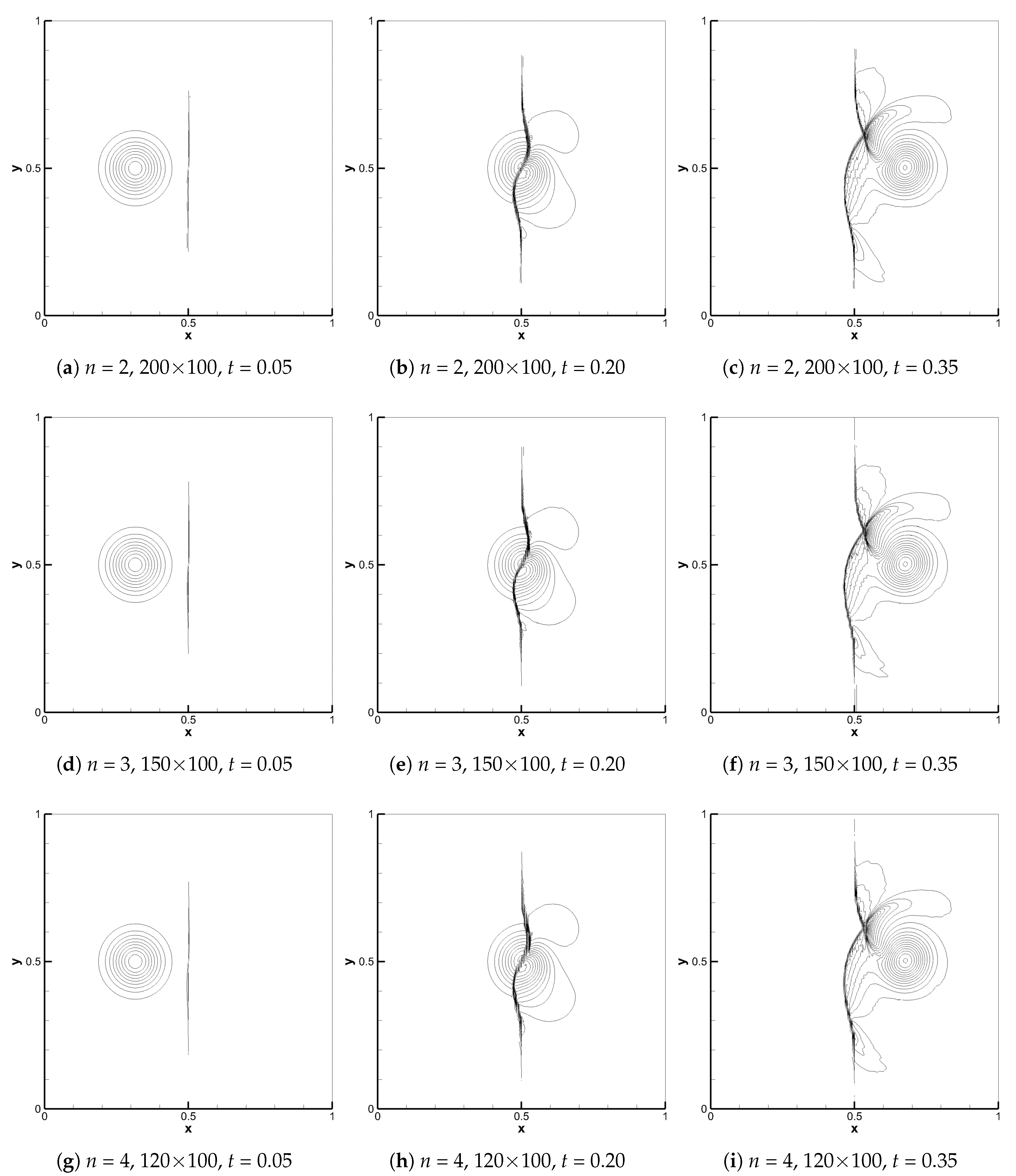
4.4. Shock–Vortex Interaction
5. Conclusions
Author Contributions
Funding
Conflicts of Interest
References
- Wang, Q.; Ren, Y.X.; Li, W. Compact high order finite volume method on unstructured grids I: Basic formulations and one-dimensional schemes. J. Comput. Phys. 2016, 314, 863–882. [Google Scholar] [CrossRef]
- Gao, X.; Owen, L.D.; Guzik, S.M. A high-order finite-volume method for combustion. In Proceedings of the AIAA Scitech 2016 Forum, San Diego, CA, USA, 4–8 January 2016; pp. 1–14. [Google Scholar]
- Lele, S.K. Compact finite difference schemes with spectral-like resolution. J. Comput. Phys. 1992, 103, 16–42. [Google Scholar] [CrossRef]
- Deng, X.; Mao, M.; Tu, G.; Zhang, H.; Zhang, Y. High-order and high accurate CFD methods and their applications for complex grid problems. Commun. Comput. Phys. 2012, 11, 1081–1102. [Google Scholar] [CrossRef]
- Allahyari, M.; Mohseni, K. Numerical simulation of flows with shocks and turbulence using observable methodology. In Proceedings of the AIAA Scitech 2018 Forum, Kissimmee, FL, USA, 8–12 January 2018; pp. 1–10. [Google Scholar]
- Jause-Labert, C.; Godeferd, F.; Favier, B. Numerical validation of the volume penalization method in three-dimensional pseudo-spectral simulations. Comput. Fluids 2012, 67, 41–56. [Google Scholar] [CrossRef]
- Shu, C.W. Essentially non-oscillatory and weighted essentially non-oscillatory schemes for hyperbolic conservation laws. In Advanced Numerical Approximation of Nonlinear Hyperbolic Equations; Springer: Berlin/Heidelberg, Germany, 1998; pp. 325–442. [Google Scholar]
- van der Weide, E.; Giangaspero, G.; Svärd, M. Efficiency benchmarking of an energy stable high-order finite difference discretization. AIAA J. 2015, 53, 1845–1860. [Google Scholar] [CrossRef]
- Reed, W.; Hill, T. Triangular Mesh Methods for the Neutron Transport Equation; Technical Report LA-UR-73-479; Los Alamos Scientific Laboratory: Los Alamos, NM, USA, 1973. [Google Scholar]
- Cockburn, B.; Shu, C.W. The Runge–Kutta local projection P1-discontinuous Galerkin finite element method for scalar conservation laws. Math. Model. Numer. Anal. 1991, 25, 337–361. [Google Scholar] [CrossRef]
- Cockburn, B.; Shu, C.W. TVB Runge-Kutta local projection discontinuous Galerkin finite element method for conservation laws II: General framework. Math. Comput. 1989, 52, 411–435. [Google Scholar]
- Cockburn, B.; Lin, S.Y.; Shu, C.W. TVB Runge-Kutta local projection discontinuous Galerkin finite element method for conservation laws III: One-dimensional systems. J. Comput. Phys. 1989, 84, 90–113. [Google Scholar] [CrossRef]
- Cockburn, B.; Hou, S.; Shu, C.W. The Runge-Kutta local projection discontinuous Galerkin finite element method for conservation laws. IV: The multidimensional case. Math. Comput. 1990, 54, 545–581. [Google Scholar]
- Cockburn, B.; Shu, C.W. The Runge–Kutta discontinuous Galerkin method for conservation laws V: Multidimensional systems. J. Comput. Phys. 1998, 141, 199–224. [Google Scholar] [CrossRef]
- Hesthaven, J.S.; Warburton, T. Nodal Discontinuous Galerkin Methods: Algorithms, Analysis, and Applications, 1st ed.; Springer: New York, NY, USA, 2008. [Google Scholar]
- Atkins, H.L.; Pampell, A. Robust and accurate shock capturing method for high-order discontinuous Galerkin methods. In Proceedings of the 20th AIAA Computational Fluid Dynamics Conference, Honolulu, HI, USA, 27–30 June 2011; pp. 1–22. [Google Scholar]
- Barter, G.; Darmofal, D. Shock capturing with higher-order, PDE-based artificial viscosity. In Proceedings of the 18th AIAA Computational Fluid Dynamics Conference, Miami, FL, USA, 25–28 June 2007; pp. 1–14. [Google Scholar]
- Burbeau, A.; Sagaut, P.; Bruneau, C.H. A problem-independent limiter for high-order Runge-Kutta discontinuous Galerkin methods. J. Comput. Phys. 2001, 169, 111–150. [Google Scholar] [CrossRef]
- Clain, S.; Diot, S.; Loubère, R. A high-order finite volume method for systems of conservation laws—Multi -dimensional optimal order detection (MOOD). J. Comput. Phys. 2011, 230, 4028–4050. [Google Scholar] [CrossRef]
- Dumbser, M.; Loubère, R. A simple robust and accurate a posteriori sub-cell finite volume limiter for the discontinuous Galerkin method on unstructured meshes. J. Comput. Phys. 2016, 319, 163–199. [Google Scholar] [CrossRef]
- Klöckner, A.; Warburton, T.; Hesthaven, J.S. Viscous shock capturing in a time-explicit discontinuous Galerkin method. Math. Model. Nat. Phenom. 2011, 6, 57–83. [Google Scholar] [CrossRef]
- Lv, Y.; See, Y.C.; Ihme, M. An entropy-residual shock detector for solving conservation laws using high-order discontinuous Galerkin methods. J. Comput. Phys. 2016, 322, 448–472. [Google Scholar] [CrossRef]
- Nguyen, C.; Peraire, J. An adaptive shock-capturing HDG method for compressible flows. In Proceedings of the 20th AIAA Computational Fluid Dynamics Conference, Honolulu, HI, USA, 27–30 June 2011; pp. 1–20. [Google Scholar]
- Persson, P.O.; Peraire, J. Sub-cell shock capturing for discontinuous Galerkin methods. In Proceedings of the 44th AIAA Aerospace Sciences Meeting and Exhibit, Reno, NV, USA, 9–12 January 2006; pp. 1–13. [Google Scholar]
- Sheshadri, A. An analysis of stability of the flux reconstruction formulation with applications to shock capturing. Ph.D. Thesis, Stanford University, Stanford, CA, USA, 2016. [Google Scholar]
- Vuik, M.J.; Ryan, J.K. Multiwavelet troubled-cell indicator for discontinuity detection of discontinuous Galerkin schemes. J. Comput. Phys. 2014, 270, 138–160. [Google Scholar] [CrossRef]
- Choi, J.H.; Alonso, J.J.; van der Weide, E. Simple shock detector for discontinuous Galerkin method. In Proceedings of the AIAA Scitech 2019 Forum, San Diego, CA, USA, 7–11 January 2019. [Google Scholar]
- Roe, P.L. Approximate Riemann solvers, parameter vectors, and difference schemes. J. Comput. Phys. 1981, 43, 357–372. [Google Scholar] [CrossRef]
- Lax, P.D. Weak solutions of nonlinear hyperbolic equations and their numerical computation. Commun. Pure Appl. Math. 1954, 7, 159–193. [Google Scholar] [CrossRef]
- Toro, E.F. Riemann Solvers and Numerical Methods for Fluid Dynamics: A Practical Introduction; Springer: Berlin/Heidelberg, Germany, 2009; Chapter 5,6,7,11. [Google Scholar]
- Toro, E.F.; Millington, R.C.; Nejad, L. Towards very high order Godunov schemes. In Godunov Methods: Theory and Applications; Springer: Boston, MA, USA, 2001; pp. 907–940. [Google Scholar]
- Dumbser, M.; Enaux, C.; Toro, E.F. Finite volume schemes of very high order of accuracy for stiff hyperbolic balance laws. J. Comput. Phys. 2008, 227, 3971–4001. [Google Scholar] [CrossRef]
- Rezzolla, L.; Zanotti, O. Relativistic Hydrodynamics; Oxford University Press: Oxford, UK, 2013. [Google Scholar]
- Zanotti, O. Discontinuous Galerkin Methods for Hyperbolic PDEs. Lecture 2. In Proceedings of the Prospects in Theoretical Physics 2016, Princeton, NJ, USA, 18–29 July 2016; pp. 1–59. Available online: https://static.ias.edu/pitp/2016/node/1026.html (accessed on 10 July 2019).
- Sod, G. Survey of several finite difference methods for systems of nonlinear hyperbolic conservation laws. J. Comput. Phys. 1978, 27, 1–31. [Google Scholar] [CrossRef]
- Shu, C.W.; Osher, S. Efficient implementation of essentially non-oscillatory shock-capturing schemes II. J. Comput. Phys. 1989, 83, 32–78. [Google Scholar] [CrossRef]
- Jiang, G.S.; Shu, C.W. Efficient Implementation of Weighted ENO Schemes. J. Comput. Phys. 1996, 126, 202–228. [Google Scholar] [CrossRef]
- SU2, The Open-Source CFD Code. Available online: https://su2code.github.io (accessed on 1 June 2019).


| Grid Level | Element Length | n = 2 | n = 3 | n = 4 | |||
|---|---|---|---|---|---|---|---|
| Filtering | W/O Filtering | Filtering | W/O Filtering | Filtering | W/O Filtering | ||
| 1 | 10/4 | 2.112E-02 | 2.112E-02 | 2.708E-02 | 2.708E-02 | 1.332E-02 | 1.332E-02 |
| 2 | 10/6 | 1.598E-02 | 1.598E-02 | 1.422E-02 | 1.422E-02 | 4.114E-03 | 4.114E-03 |
| 3 | 10/8 | 9.339E-03 | 9.339E-03 | 6.474E-03 | 6.474E-03 | 1.135E-03 | 1.135E-03 |
| 4 | 10/12 | 3.376E-03 | 3.376E-03 | 1.179E-03 | 1.179E-03 | 1.434E-04 | 1.434E-04 |
| 5 | 10/16 | 1.843E-03 | 1.843E-03 | 3.415E-04 | 3.415E-04 | 3.417E-05 | 3.417E-05 |
| Grid Level | Element Length | n = 2 | n = 3 | n = 4 | |||
|---|---|---|---|---|---|---|---|
| Filtering | W/O Filtering | Filtering | W/O Filtering | Filtering | W/O Filtering | ||
| 1 | 10/4 | 3.535E-02 | 3.931E-02 | 2.580E-02 | 2.580E-02 | 1.815E-02 | 1.815E-02 |
| 2 | 10/6 | 1.643E-02 | 1.648E-02 | 1.130E-02 | 1.130E-02 | 6.296E-03 | 6.296E-03 |
| 3 | 10/8 | 1.300E-02 | 1.251E-02 | 6.668E-03 | 6.668E-03 | 1.033E-03 | 1.033E-03 |
| 4 | 10/12 | 5.167E-03 | 5.167E-03 | 2.611E-03 | 2.611E-03 | 1.440E-04 | 1.440E-04 |
| 5 | 10/16 | 2.099E-03 | 2.099E-03 | 8.461E-04 | 8.461E-04 | 3.923E-05 | 3.923E-05 |
© 2019 by the authors. Licensee MDPI, Basel, Switzerland. This article is an open access article distributed under the terms and conditions of the Creative Commons Attribution (CC BY) license (http://creativecommons.org/licenses/by/4.0/).
Share and Cite
Choi, J.H.; Alonso, J.J.; van der Weide, E. A Simple and Robust Shock-Capturing Approach for Discontinuous Galerkin Discretizations. Energies 2019, 12, 2651. https://doi.org/10.3390/en12142651
Choi JH, Alonso JJ, van der Weide E. A Simple and Robust Shock-Capturing Approach for Discontinuous Galerkin Discretizations. Energies. 2019; 12(14):2651. https://doi.org/10.3390/en12142651
Chicago/Turabian StyleChoi, Jae Hwan, Juan J. Alonso, and Edwin van der Weide. 2019. "A Simple and Robust Shock-Capturing Approach for Discontinuous Galerkin Discretizations" Energies 12, no. 14: 2651. https://doi.org/10.3390/en12142651
APA StyleChoi, J. H., Alonso, J. J., & van der Weide, E. (2019). A Simple and Robust Shock-Capturing Approach for Discontinuous Galerkin Discretizations. Energies, 12(14), 2651. https://doi.org/10.3390/en12142651