Adaptive Integral Backstepping Controller for PMSM with AWPSO Parameters Optimization

Abstract

This article presents an adaptive integral backstepping controller (AIBC) for permanent magnet synchronous motors (PMSMs) with adaptive weight particle swarm optimization (AWPSO) parameters optimization. The integral terms of dq axis current following errors are introduced into the control law, and by constructing an appropriate Lyapunov function, the adaptive law with the differential term and the control law with the integral terms of the current error are derived to weaken the influence of internal parameters perturbation on current control. The AWPSO algorithm is used to optimize the parameters of the AIBC. Based on the analysis of single-objective optimization and multi-objective realization process, a method for transforming multi-objective optimization with convex Prato frontier into single-objective optimization is presented. By this method, a form of fitness function suitable for parameters optimization of backstepping controller is determined, and according to the theoretical derivation and large number of simulation results, the corresponding parameters of the optimization algorithm are set. By randomly adjusting the inertia weight and changing the acceleration factor, the algorithm can accelerate the convergence speed and solve the problem of parameters optimization of the AIBC. The feasibility and effectiveness of the proposed controller for PMSM are verified by simulation and experimental studies.

1. Introduction

Permanent magnet synchronous motors (PMSMs) have been widely applied in various fields due to their simple structure, high power density and reliable operation [1,2,3,4]. However, due to their nonlinearity, strong coupling, and real-time changes of stator resistance, inductance and load torque during its operation, it is difficult to achieve the control performance requirements by using general linear control methods (such as PI control) [5,6]. In recent years, with the development of control theory, some nonlinear control methods have been applied to PMSM, such as sliding mode control (SMC) [7,8,9,10], feedback linearization control (FLC) [11,12,13], auto disturbance rejection control (ADRC) [14,15,16,17], and backstepping control (BC) [18,19,20]. Among them, the backstepping control method has attracted much attention because it is easy to combine with adaptive parameters estimation technology to weaken the influence of system uncertainties [21,22].

In the early 1990s, Kokotovic, et al. [23] put forward the backstepping control method, which provides a feasible design method and ideas for the design of nonlinear controllers. Backstepping control is a systematic cyclic design method. Based on Lyapunov stability theory, the control law and adaptive law satisfying the convergence condition of Lyapunov function are derived by constructing feedback control law and Lyapunov function simultaneously. The theory of backstepping control has attracted wide attention in the field of motor control, because it can not only achieve complete decoupling of PMSM system, but also simplify the design process [24,25]. In order to ensure better stability and dynamic performance of the system, the adaptive backstepping control (ABC) method which combines the backstepping design method with the adaptive control method is generally used for nonlinear uncertain systems [26,27,28,29]. The adaptive control law is constructed while the feedback control law and Lyapunov function are constructed, which not only meets the requirements of system stability, but also reduces the design steps and design burden. For PMSM control system, the adaptive backstepping design method is usually used to design the controller [30]. In [31], an adaptive backstepping controller for PMSM is designed with inductance of dq axis and load torque as uncertainties. The simulation results show that the designed controller can track the input reference speed well, and is robust to parameters uncertainties and load disturbance. However, the control law and adaptive law designed in this paper are complex and unsuitable for engineering applications. In [32], the backstepping control strategy is applied to the speed tracking system of PMSM, which simplifies the design process of general system, reduces the number of adjusting parameters in the system control, guarantees the global stability of the system and achieves good speed tracking, but it does not consider the influence of the change of parameters on the system performance. In [33], adaptive control and backstepping control are combined and applied to speed tracking system of PMSMs with uncertain parameters. This method aims at the real-time estimation of resistance and load in the control system and achieves disturbance suppression to a certain extent. However, it does not consider the influence of the parameters selection of speed backstepping regulator on the performance of the system. Because the selection of parameters in the system design has a great influence on the stability and dynamic performance of the system, it is very important to select the parameters of backstepping regulator in the control system of PMSM.

In summary, advanced control theory has achieved a lot of research results in the field of PMSM control. Among them, backstepping control can effectively improve the dynamic and static performance of PMSM, and gradually develop in the field of PMSM control. However, there still exist some problems to be studied, mainly in the following two aspects:

(1) It is necessary to further improve the robustness of the backstepping control algorithm. Due to its own characteristics and environment impact, the load torque and dq axis inductance of PMSM will change in real time. However, it is difficult to deduce the adaptive law because the inductance of dq axis are coupled with each other in the mathematical model [34,35]. Therefore, it is difficult to observe the inductance uncertainties of the dq axis by designing an observer. Because of the inductance uncertainties of dq axis, the current control of dq axis becomes worse, and even the motor control system may collapse.

(2) There is no standard method for parameters tuning of backstepping control algorithm. According to Lyapunov function, only the lower limit of each parameter can be determined, but the exact value of parameters cannot be obtained. Especially when there are many parameters in the controller, the tuning of various parameters becomes particularly difficult [36]. In the controller design, the parameters selection can only be determined by experience and a lot of debugging. The parameters of backstepping controller are usually selected as fixed constant, which limits the dynamic performance of the system to a certain extent. Aiming at this problem, it is popular to combine adaptive backstepping control with fuzzy control to adjust the parameters online [37,38,39,40]. However, the adaptive controllers mentioned in these references have fewer parameters to be tuned or only adjust the selected fewer parameters online. When there are many parameters to be tuned in the control system, the parameters optimization of the controller becomes a typical high-dimensional nonlinear optimization problem, and then the fuzzy control will no longer be applicable. What’s more, fuzzy adaptive adjustment is to dynamically adjust inertia weight by using fuzzy reasoning system, but it is difficult to establish membership function and fuzzy rules.

In view of the above two major problems, the main contribution of this article is to present an adaptive integral backstepping controller (AIBC) for PMSM with adaptive weight particle swarm optimization (AWPSO) parameters optimization, which effectively suppress the influence of load torque disturbance and inductance uncertainties of the dq axis on the system, and the parameters tuning problem of the controller is effectively solved. The innovations of this article mainly include: (1) Aiming at the load torque disturbance and inductance uncertainties of the dq axis, based on the function of differential and integral in control system, an AIBC with differential term for PMSM is proposed. (2) Aiming at the parameters tuning problem of the AIBC with differential term, an AWPSO algorithm for controller parameters optimization and the rules for selecting adaptive weight, acceleration factor and fitness function are proposed. The feasibility and effectiveness of the proposed controller for PMSM are verified by simulation and experimental studies.

2. Design of the AIBC with Differential Term for PMSM

2.1. Design of Adaptive Backstepping Controller with Differential Term

According to field oriented control theory, the mathematical model of PMSM in dq axis can be expressed as:

$$\left[\begin{array}{c}{u}_q\\ u_d\end{array}\right]=\left[\begin{array}{cc}{R}_s+p{L}_q& n_p{\omega }_r{L}_d\\ -n_p{\omega }_r{L}_q& R_s+p{L}_d\end{array}\right]\left[\begin{array}{c}{i}_q\\ i_d\end{array}\right]+\left[\begin{array}{c}{n}_p{\omega }_r{\psi }_f\\ 0\end{array}\right]$$

(1)

where $i_d$ and $i_q$ are the current of dq axis, $u_d$ and $u_q$ are the voltage of dq axis, $L_d$ and $L_q$ are the stator inductance of dq axis, $R_s$ is the stator resistance, ${\omega }_r$ is the mechanical angular speed of the rotor, $n_p$ is the number of pole pairs, and ${\psi }_f$ is the rotor flux.

Transform (1) into:

$$\{\begin{array}{l}{\dot{i}}_d=\frac{u_d}{L_d}-\frac{R_s}{L_d}{i}_d+n_p{\omega }_r\frac{L_q}{L_d}{i}_q\\ {\dot{i}}_q=\frac{u_q}{L_q}-\frac{R_s}{L_q}{i}_q-n_p{\omega }_r\frac{L_d}{L_q}{i}_d-n_p{\omega }_r\frac{{\psi }_f}{L_q}\end{array}$$

(2)

The electromagnetic torque expression of PMSM is as follows:

$$T_e=\frac{3n_p}{2}\left[{\psi }_f{i}_q+\left(L_d-L_q\right)i_d{i}_q\right]$$

(3)

The equation of mechanical motion is:

$$T_e=T_L+B{\omega }_r+J\frac{d{\omega }_r}{dt}$$

(4)

where $T_e$ is the output electromagnetic torque, $T_L$ is the load torque, $J$ is the moment of inertia, $B$ is the viscous friction coefficient. Combine (3) with (4),

$${\dot{\omega }}_r=\frac{3n_p{\psi }_f}{2J}{i}_q+\frac{3n_p}{2J}\left(L_d-L_q\right)i_d{i}_q-\frac{B}{J}{\omega }_r-\frac{1}{J}{T}_L$$

(5)

Considering (5) as the first subsystem and (2) as the second, the PMSM control system is a nonlinear system composed of speed control subsystem and current control subsystem. Therefore, the backstepping control method can be used to design the speed controller of PMSM. The specific design steps are as follows:

Step 1: Define the reference speed as ${\omega }_r^{*}$, then the speed following error is:

$$e_{\omega }={\omega }_r^{\ast }-{\omega }_r$$

(6)

The derivative of (6) is:

$${\dot{e}}_{\omega }=\frac{1}{J}\left[T_L+B{\omega }_r-\frac{3n_p}{2}{\psi }_f{i}_q-\frac{3n_p}{2}\left(L_d-L_q\right)i_d{i}_q\right]$$

(7)

Define Lyapunov function as:

$$V_1=\frac{e_{\omega }^2}{2}$$

(8)

The derivative of (8) is:

$${\dot{V}}_1=e_{\omega }{\dot{e}}_{\omega }=\frac{e_{\omega }}{J}\left(B{\omega }_r+T_L\right)-\frac{3n_p}{2J}{e}_{\omega }\left[{\psi }_f{i}_q+\left(L_d-L_q\right)i_d{i}_q\right]$$

(9)

Define $k_{\omega }$ as speed feedback gain, take positive constant, then (9) is converted to:

$${\dot{V}}_1=-k_{\omega }{e}_{\omega }^2+\frac{e_{\omega }}{J}\left[T_L+B{\omega }_r-\frac{3n_p}{2}\left(L_d-L_q\right)i_d{i}_q-\frac{3n_p}{2}{\psi }_f{i}_q+k_{\omega }J{e}_{\omega }\right]$$

(10)

$T_L$ and $J$ are considered as uncertain parameters for estimation, and ideal virtual control variables $i_d^{*}$ and $i_q^{*}$ are defined as:

$$\{\begin{array}{l}{i}_d^{\ast }=0\\ i_q^{\ast }=\frac{2}{3n_p{\psi }_f}\left({\widehat{T}}_L+B{\omega }_r+k_{\omega }\widehat{J}{e}_{\omega }\right)\end{array}$$

(11)

where ${\widehat{T}}_L$ and $\widehat{J}$ are load torque and inertia estimation respectively. If (11) is added to (7), the speed error can be reorganized into the following equation:

$${\dot{e}}_{\omega }=\frac{1}{J}\left(-{\tilde{T}}_L+\frac{3n_p}{2}{\psi }_f{e}_q+\frac{3n_p}{2}\left(L_d-L_q\right)e_d{i}_q-k_{\omega }\widehat{J}{e}_{\omega }\right)$$

(12)

where ${\tilde{T}}_L={\widehat{T}}_L-T_L$. Define the dq axis current error $e_d$, $e_q$ as:

$$\{\begin{array}{l}{e}_d=i_d^{\ast }-i_d\\ e_q=i_q^{\ast }-i_q\end{array}$$

(13)

The dq axis current error are derived, then:

$$\{\begin{array}{l}{\dot{e}}_d=\frac{R_s{i}_d-n_p{\omega }_r{L}_q{i}_q-u_d}{L_d}\\ {\dot{e}}_q=\frac{2\left(k_{\omega }\widehat{J}-B\right)}{3n_p{\psi }_{f}J}\left[\frac{3n_p{\psi }_f}{2}{e}_q+\frac{3n_p}{2}\left(L_d-L_q\right)e_d{i}_q-k_{\omega }\widehat{J}{e}_{\omega }\right]-\frac{2\left(k_{\omega }\widehat{J}-B\right)}{3n_p{\psi }_{f}J}{\tilde{T}}_L+\frac{R_s{i}_q+n_p{\omega }_r{L}_d{i}_d+n_p{\omega }_r{\psi }_f-u_q}{L_q}\end{array}$$

(14)

Step 2: In order to make the differential term of the q axis current error appear in the derived adaptive law, the Lyapunov function is defined as:

$$V=V_1+\frac{1}{2}{e}_d^2+\frac{1}{2}{e}_q^2+\frac{1}{2{\gamma }_1}{\left({\tilde{T}}_L+k_{m}J{e}_q\right)}^2+\frac{1}{2{\gamma }_2}{\tilde{J}}^2$$

(15)

where ${\gamma }_1$ and ${\gamma }_2$ are adaptive gains, and they are positive constants, $\tilde{J}=\widehat{J}-J$ is the estimation error of moment of inertia, $k_m$ is the differential gain of q axis current. Derive (15), then:

$$\begin{array}{ll}\dot{V}& =e_{\omega }{\dot{e}}_{\omega }+e_d{\dot{e}}_d+e_q{\dot{e}}_q+\frac{1}{{\gamma }_1}\tilde{J}\dot{\tilde{J}}+\frac{1}{{\gamma }_2}\left({\tilde{T}}_L+k_{m}J{e}_q\right)\left({\dot{\tilde{T}}}_L+k_{m}J{\dot{e}}_q\right)\\ & =-k_{\omega }{e}_{\omega }^2-k_d{e}_d^2-k_q{e}_q^2+e_d\left[\frac{R_s{i}_d-n_p{\omega }_r{L}_q{i}_q-u_d}{L_d}+\frac{3n_p}{2J}\left(L_d-L_q\right)e_{\omega }{i}_q+k_d{e}_d\right]\\ & +e_q[\frac{2\left(k_{\omega }J-B\right)}{3n_p{\psi }_{f}J}\alpha -\frac{2\left(k_{\omega }\widehat{J}-B\right)}{3n_p{\psi }_{f}J}{k}_{\omega }\widehat{J}{e}_{\omega }+\frac{2k_m\left(k_{\omega }J-B\right)}{3n_p{\psi }_f}{e}_q+k_m{e}_{\omega }+\frac{3n_p{\psi }_f}{2J}{e}_{\omega }+k_q{e}_q\\ & +\frac{R_s{i}_q+n_p{\omega }_r{L}_d{i}_d+n_p{\omega }_r{\psi }_f-u_q}{L_q}]+\tilde{J}\left[\frac{1}{{\gamma }_2}\dot{\tilde{J}}-\frac{k_{\omega }}{J}{e}_{\omega }^2+\frac{2k_{\omega }{k}_m}{3n_p{\psi }_f}{e}_q^2+\frac{2k_{\omega }{e}_q}{3n_p{\psi }_{f}J}\alpha \right]+\\ & \left({\tilde{T}}_L+k_{m}J{e}_q\right)\left[\frac{1}{{\gamma }_1}\left({\dot{\tilde{T}}}_L+k_{m}J{\dot{e}}_q\right)-\frac{e_{\omega }}{J}-\frac{2\left(k_{\omega }\widehat{J}-B\right)}{3n_p{\psi }_{f}J}{e}_q\right]\end{array}$$

(16)

where $\alpha =\frac{3n_p{\psi }_f}{2}{e}_q+\frac{3n_p}{2}(L_d-L_q)e_d{i}_q$, $k_d$ and $k_q$ are positive constants. In order to ensure the global asymptotic stability of the system, the actual control laws and adaptive law are selected as:

$$\{\begin{array}{ll}{u}_d& =R_s{i}_d-n_p{\omega }_r{L}_q{i}_q+\frac{3n_p}{2J}\left(L_d-L_q\right)L_d{e}_{\omega }{i}_q+k_d{L}_d{e}_d\\ u_q& =R_s{i}_q+n_p{\omega }_r{L}_d{i}_d+n_p{\omega }_r{\psi }_f+k_q{L}_q{e}_q+L_q{k}_m{e}_{\omega }+\frac{2L_q}{3n_p{\psi }_{f}J}\left(k_{\omega }J-B\right)\left[\frac{3n_p{\psi }_f}{2}{e}_q+\frac{3n_p}{2}\left(L_d-L_q\right)e_d{i}_q\right]\\ & -\frac{2k_{\omega }\left(k_{\omega }\widehat{J}-B\right)L_q}{3n_p{\psi }_{f}J}\widehat{J}{e}_{\omega }+\frac{2k_m\left(k_{\omega }J-B\right)L_q}{3n_p{\psi }_f}{e}_q+\frac{3n_p{L}_q}{2J}{\psi }_f{e}_{\omega }\end{array}$$

(17)

$$\{\begin{array}{l}{\dot{\tilde{T}}}_L={\gamma }_1\left[\frac{e_{\omega }}{J}+\frac{2\left(k_{\omega }\widehat{J}-B\right)}{3n_p{\psi }_{f}J}{e}_q\right]-k_{m}J{\dot{e}}_q\\ \dot{\tilde{J}}=-{\gamma }_2\left\{-\frac{k_{\omega }{e}_{\omega }^2}{J}+\frac{2k_{\omega }{k}_m}{3n_p{\psi }_f}{e}_q^2\right\}-{\gamma }_2\left\{\frac{2k_{\omega }{e}_q}{3n_p{\psi }_{f}J}\left[\frac{3n_p{\psi }_f}{2}{e}_q+\frac{3n_p}{2}\left(L_d-L_q\right)e_d{i}_q\right]\right\}\end{array}$$

(18)

Introduce the above control law and adaptive law into (16), then:

$$\dot{V}=-k_{\omega }{e}_{\omega }^2-k_d{e}_d^2-k_q{e}_q^2$$

(19)

Because $k_{\omega }>0$, $k_d>0$ and $k_q>0$, then $\dot{V}\le 0$. According to Lyapunov asymptotic stability theorem, the system is asymptotically stable.

2.2. Design of the AIBC

Equation (1) is an ideal mathematical model of a PMSM, without considering the factors such as damper winding and harmonics of motor rotor. However, in the process of motor operation, the error in dq axis inductances measurement of damped windings seriously affect the control effect of dq axis current, and may even cause the collapse of motor control system. For such problem, uncertainties can generally be observed by designing observers. However, from (2), it can be seen that the dq axis inductances exist on the denominator of their current equation respectively, and are coupled with each other, so it is difficult to deduce the adaptive law. In this section, the error integrals of dq axis current are introduced into the control law, and the AIBC for PMSM is designed to reduce the error of dq axis current and the influence of parameters uncertainty on the system.

Define ${\theta }_d$ as the integral of d axis current error, ${\theta }_d={\displaystyle {\int }_0^t{e}_d(\tau )}d\tau$, ${\theta }_q$ as the integral of q axis current error, ${\theta }_q={\displaystyle {\int }_0^t{e}_q(\tau )}d\tau$, and Lyapunov function as:

$$V=\frac{1}{2}{e}_{\omega }^2+\frac{1}{2}{e}_d^2+\frac{1}{2}{e}_q^2+\frac{1}{2}{k}_{di}{\theta }_d^2+\frac{1}{2}{k}_{qi}{\theta }_q^2+\frac{1}{2{\gamma }_1}{\tilde{T}}_L^2+\frac{1}{2{\gamma }_2}{\tilde{J}}^2$$

(20)

where $k_{di}$ and $k_{qi}$ are integral gains of dq axis current respectively, and $k_{di}>0$,$k_{qi}>0$. Derive (20), then:

$$\begin{array}{ll}\dot{V}& =-k_{\omega }{e}_{\omega }^2-k_d{e}_d^2-k_q{e}_q^2+e_d\left[\frac{R_s{i}_d-n_p{\omega }_r{L}_q{i}_q-u_d}{L_d}+\frac{3n_p}{2J}\left(L_d-L_q\right)e_{\omega }{i}_q+k_d{e}_d+k_{di}{\theta }_d\right]\\ & +e_q\left[\frac{2\left(k_{\omega }J-B\right)}{3n_p{\psi }_{f}J}\alpha -\frac{2\left(k_{\omega }\widehat{J}-B\right)}{3n_p{\psi }_{f}J}{k}_{\omega }\widehat{J}{e}_{\omega }+\frac{3n_p{\psi }_f}{2J}{e}_{\omega }+k_q{e}_q+k_{qi}{\theta }_q+\frac{R_s{i}_q+n_p{\omega }_r{L}_d{i}_d+n_p{\omega }_r{\psi }_f-u_q}{L_q}\right]\\ & +\tilde{J}\left[\frac{1}{{\gamma }_2}\dot{\tilde{J}}-\frac{k_{\omega }}{J}{e}_{\omega }^2+\frac{2k_{\omega }{e}_q}{3n_p{\psi }_{f}J}\alpha \right]+{\tilde{T}}_L\left[\frac{1}{{\gamma }_1}{\dot{\tilde{T}}}_L-\frac{e_{\omega }}{J}-\frac{2\left(k_{\omega }\widehat{J}-B\right)}{3n_p{\psi }_{f}J}{e}_q\right]\end{array}$$

(21)

where $\alpha =\frac{3n_p{\psi }_f}{2}{e}_q+\frac{3n_p}{2}(L_d-L_q)e_d{i}_q$. In order to ensure the stability of the system, the control law and the adaptive law are selected respectively as:

$$\{\begin{array}{ll}{u}_d& =R_s{i}_d-n_p{\omega }_r{L}_q{i}_q+\frac{3n_p}{2J}\left(L_d-L_q\right)L_d{e}_{\omega }{i}_q+k_d{L}_d{e}_d+k_{di}{L}_d{\theta }_d\\ u_q& =R_s{i}_q+n_p{\omega }_r{L}_d{i}_d+n_p{\omega }_r{\psi }_f+k_q{L}_q{e}_q+k_{qi}{L}_q{\theta }_q+\frac{2L_q}{3n_p{\psi }_{f}J}\left(k_{\omega }J-B\right)\left[\frac{3n_p{\psi }_f}{2}{e}_q+\frac{3n_p}{2}\left(L_d-L_q\right)e_d{i}_q\right]\\ & -\frac{2k_{\omega }\left(k_{\omega }\widehat{J}-B\right)L_q}{3n_p{\psi }_{f}J}\widehat{J}{e}_{\omega }+\frac{3n_p{L}_q}{2J}{\psi }_f{e}_{\omega }\end{array}$$

(22)

$$\{\begin{array}{l}{\dot{\tilde{T}}}_L={\gamma }_1\left[\frac{e_{\omega }}{J}+\frac{2\left(k_{\omega }\widehat{J}-B\right)}{3n_p{\psi }_{f}J}{e}_q\right]\\ \dot{\tilde{J}}=-{\gamma }_2\left\{-\frac{k_{\omega }{e}_{\omega }^2}{J}+\frac{2k_{\omega }{e}_q}{3n_p{\psi }_{f}J}\left[\frac{3n_p{\psi }_f}{2}{e}_q+\frac{3n_p}{2}\left(L_d-L_q\right)e_d{i}_q\right]\right\}\end{array}$$

(23)

By introducing the above control law (22) and adaptive law (23) into (21), then

$$\dot{V}=-k_{\omega }{e}_{\omega }^2-k_d{e}_d^2-k_q{e}_q^2$$

(24)

Because $k_{\omega }>0$, $k_d>0$ and $k_q>0$, then $\dot{V}\le 0$. According to Lyapunov asymptotic stability theorem, the system is asymptotically stable.

2.3. Design of the Anti-Saturation Torque Observer

The backstepping control strategies mentioned above haven’t consider the constraints of the system. However, in PMSM control system, such constraints exist. For the torque observer, the estimated value should be less than the maximum load torque allowed by the motor system, i.e., $|{\widehat{T}}_L|\le T_{max}$. At the same time, it can be seen from (23) that ${\widehat{T}}_L$ contains integral term of speed error $e_{\omega }$ and q axis current error $e_q$. In the process of motor startup or speed regulation, the input values of $e_{\omega }$ and $e_q$ may be larger. Therefore, in the process of motor operation, the existence of large input signals and torque constraint lead to the integral saturation of the torque observer, which affects the dynamic performance of the system. To solve this problem, an anti-saturation integrator is introduced to enable the observer to exit the saturation state as soon as possible. Taking the torque adaptive law expressed in (18) as an example, the specific process of the algorithm is illustrated. The structure of the anti-saturation torque observer is shown in Figure 1. In the figure, $K=2{\gamma }_1/3n_p{\psi }_{f}J$.

Under unsaturated conditions:

$${\widehat{T}}_L=\widehat{T}{}_L^{\prime }={\displaystyle {\int }_0^t\frac{{\gamma }_1}{J}{e}_{\omega }\left(\tau \right)d\tau }+{\displaystyle {\int }_0^t\frac{2{\gamma }_1\left(k_{\omega }\widehat{J}-B\right)}{3n_p{\psi }_{f}J}{e}_q\left(\tau \right)d\tau }-k_{m}J{e}_q={\displaystyle {\int }_0^t\beta \left(\tau \right)d\tau }-k_{m}J{e}_q={\beta }^{\prime }-k_{m}J{e}_q$$

(25)

where $\beta =\frac{{\gamma }_1}{J}{e}_{\omega }+\frac{2{\gamma }_1\left(k_{\omega }\widehat{J}-B\right)}{3n_p{\psi }_{f}J}{e}_q$, ${\beta }^{\prime }={\displaystyle {\int }_0^t\beta \left(\tau \right)d\tau }$. When $\widehat{T}{}_L^{\prime }$ enters the positive saturation range, the observed value of the torque is the maximum value of the torque $T_{max}$, and when $\widehat{T}{}_L^{\prime }$ enters the negative saturation range, the observed value of the torque is the minimum value of the torque $T_{min}$, i.e.,:

$${\widehat{T}}_L=\{\begin{array}{l}\begin{array}{cc}{T}_{max}& \widehat{T}{}_L^{\prime }\ge T_{max}\end{array}\\ \begin{array}{cc}\widehat{T}{}_L^{\prime }& -T_{max}<\widehat{T}{}_L^{\prime }<T_{max}\end{array}\\ \begin{array}{cc}-T_{max}& \widehat{T}{}_L^{\prime }\end{array}\le -T_{max}\end{array}$$

(26)

Under this condition:

$${\beta }^{\prime }\left(t\right)={\displaystyle {\int }_0^t\left[\beta \left(\tau \right)-k_c\left(\widehat{T}{}_L^{\prime }-{\widehat{T}}_L\right)\right]d\tau }$$

(27)

where $k_c$ is the desaturation adjustment coefficient. When the torque observer is saturated and the value of $k_c$ is large, according to (27), ${\beta }^{\prime }$ will decrease rapidly, so that $\widehat{T}{}_L^{\prime }$ can withdraw from saturation state and the torque observation value can be restored to (25).

2.4. Design of the Integration Algorithm

Aiming at load disturbance and parameters uncertainty of PMSM, adaptive backstepping controller with differential term and the AIBC are designed respectively. Meanwhile, in order to avoid the problem of integration saturation, an anti-saturation integrator is introduced. These methods can be used separately or jointly according to the actual situation. Under the combined use, the motor control system has better anti-interference ability and dynamic characteristic.

2.4.1. Design of the AIBC with Differential Term

The Lyapunov function is defined as:

$$V=\frac{1}{2}{e}_{\omega }^2+\frac{1}{2}{e}_d^2+\frac{1}{2}{e}_q^2+\frac{1}{2}{k}_{di}{\theta }_d^2+\frac{1}{2}{k}_{qi}{\theta }_q^2+\frac{1}{2{\gamma }_1}{({\tilde{T}}_L+k_{m}J{e}_q)}^2+\frac{1}{2{\gamma }_2}{\tilde{J}}^2$$

(28)

In order to ensure the stability of the system, the control law and the adaptive law are selected respectively as:

$$\{\begin{array}{ll}{u}_d& =R_s{i}_d-n_p{\omega }_r{L}_q{i}_q+\frac{3n_p}{2J}\left(L_d-L_q\right)L_d{e}_{\omega }{i}_q+k_d{L}_d{e}_d+k_{di}{L}_d{\theta }_d\\ u_q& =R_s{i}_q+n_p{\omega }_r{L}_d{i}_d+n_p{\omega }_r{\psi }_f+k_q{L}_q{e}_q+k_q{L}_m{e}_{\omega }+k_{qi}{L}_q{\theta }_q+\frac{2L_q}{3n_p{\psi }_{f}J}\left(k_{\omega }J-B\right)\left[\frac{3n_p{\psi }_f}{2}{e}_q+\frac{3n_p}{2}\left(L_d-L_q\right)e_d{i}_q\right]\\ & -\frac{2k_{\omega }\left(k_{\omega }\widehat{J}-B\right)L_q}{3n_p{\psi }_{f}J}\widehat{J}{e}_{\omega }+\frac{3n_p{L}_q}{2J}{\psi }_f{e}_{\omega }+\frac{2k_m\left(k_{\omega }J-B\right)L_q}{3n_p{\psi }_f}{e}_q\end{array}$$

(29)

$$\{\begin{array}{l}{\dot{\tilde{T}}}_L={\gamma }_1\left[\frac{e_{\omega }}{J}+\frac{2\left(k_{\omega }\widehat{J}-B\right)}{3n_p{\psi }_{f}J}{e}_q\right]-k_{m}J{\dot{e}}_q\\ \dot{\tilde{J}}=-{\gamma }_2\left\{-\frac{k_{\omega }{e}_{\omega }^2}{J}+\frac{2k_{\omega }{k}_m}{3n_p{\psi }_f}{e}_q^2+\frac{2k_{\omega }{e}_q}{3n_p{\psi }_{f}J}\left[\frac{3n_p{\psi }_f}{2}{e}_q+\frac{3n_p}{2}\left(L_d-L_q\right)e_d{i}_q\right]\right\}\end{array}$$

(30)

2.4.2. System Stability Analysis

According to (28), it is known that $V(e_{\omega },e_q,e_d)$ is positive definite, and it has infinite upper bound. By introducing the above control law (29) and adaptive law (30) into $\dot{V}(e_{\omega },e_q,e_d)$, then:

$$\dot{V}=-k_{\omega }{e}_{\omega }^2-k_d{e}_d^2-k_q{e}_q^2$$

(31)

When $k_{\omega }$, $k_d$, and $k_q$ are positive constant, $\dot{V}\le 0$. Then $V(e_{\omega }(t),e_q(t),e_d(t))\le V(e_{\omega }(0),e_q(0),e_d(0))$, Considering that $V(e_{\omega }(0),e_q(0),e_d(0))$ is bounded, then $V(e_{\omega }(t),e_q(t),e_d(t))$ is non-incremental bounded. Thus

$$\underset{t\to \infty }{\lim }{\displaystyle {\int }_0^t\dot{V}\left(e_{\omega }\left(\tau \right),e_q\left(\tau \right),e_d\left(\tau \right)\right)}d\tau <\infty$$

(32)

Because $\ddot{V}=-2k_{\omega }{e}_{\omega }{\dot{e}}_{\omega }-2k_d{e}_d{\dot{e}}_d-2k_q{e}_q{\dot{e}}_q$, and ${\dot{e}}_{\omega }$, ${\dot{e}}_d$, ${\dot{e}}_q$, $e_{\omega }$, $e_d$, $e_q$ are all bounded. So $\ddot{V}$ is bounded, and $\dot{V}$ is uniformly continuous. According to Lyapunov lemma, when $t\to \infty$, $\dot{V}(t)\to 0$. According to Barbalat lemma, $e_{\omega }$, $e_d$ and $e_q$ all converge to zero, i.e.,:

$$\{\begin{array}{l}\underset{t\to \infty }{\lim }{\omega }_r\left(t\right)={\omega }_r^{\ast }\\ \underset{t\to \infty }{\lim }{i}_q\left(t\right)=i_q^{\ast }\\ \underset{t\to \infty }{\lim }{i}_d\left(t\right)=i_d^{\ast }\end{array}$$

(33)

After the above analysis, the designed AIBC with differential term can make the system globally asymptotically stable, and the tracking error approache zero, so as to achieve the target of speed and current tracking.

3. Design of AWPSO for Parameters Optimization of the AIBC with Differential Term

The AIBC with differential term can better restrain the influence of load torque disturbance and inductances uncertainty on the system. However, due to the introduction of differential and integral terms, the controller parameters are increased ($k_{\omega }$, $k_q$, $k_d$, $k_{qi}$, $k_{di}$, $k_m$, ${\gamma }_1$, ${\gamma }_2$), which makes debugging difficult. To solve this problem, this section adopts AWPSO optimization algorithm to optimize the parameters of the AIBC with differential terms.

3.1. Principle of AWPSO Algorithm

Inertial weight ($w$) and acceleration factors ($c_1$,$c_2$) directly affect the local search ability, global search ability and convergence speed of particle swarm optimization (PSO). In the early stages of PSO research, $w$ was assigned a fixed value. Later, with the deepening of the research, the mechanism of changing $w$ dynamically was introduced. The main methods to change $w$ are random adjustment, linear decline, nonlinear decline, fuzzy adaptive, chaotic decline and so on. Random adjustment means that each iteration $w$ is a random value, which can make the population have a chance to obtain smaller $w$ in the early stage of search, strengthen its local search, and obtain larger $w$ in the later stage of search, so as to obtain stronger global search ability. Linear decline, nonlinear decline and chaotic decline mean that $w$ decreases gradually with the increase of iteration times. However, this method is also easy to make particles miss the optimal point at the beginning of the search because of its weak local search ability, and easily fall into the local extreme value at the later stage. Fuzzy adaptive adjustment is to dynamically adjust inertia weight by using fuzzy reasoning system, but it is difficult to establish membership function and fuzzy rules.

$c_1$ and $c_2$ are usually determined by experience. It is generally believed that when $c_1\approx c_2=2$, the working efficiency of particles is the highest. At this time, the local search ability and the global search ability reach a balance state, and the particles are attracted to the average of the optimal position of the particles $p_i$ and the optimal position of the population $p_g$. In 2004, Mahfouf et al. [41]. proposed a particle swarm optimization method with adaptive inertia weight. The velocity and location updating formula are as follows:

$$v_i(t+1)=w{v}_i(t)+\alpha r_1\left[p_i-x_i(t)\right]+\alpha r_2\left[p_g-x_i(t)\right]$$

(34)

$$x_i(t+1)=x_i(t)+v_i(t+1)$$

(35)

where $t=1,2,...,T_{\max }$ is the number of iterations, and $T_{\max }$ is the maximum number of iterations. $i=1,2,...,N$, and $N$ is the number of individual particles in population. $v_i(t)$ is the velocity of particle $i$ in $t$ times iteration, and $x_i(t)$ is the location of particle $i$ in $t$ times iteration. $r_1$ is the random number between 0 and 1. The values of $c_1$ and $c_2$ are $\alpha$, and $\alpha$ is defined as:

$$\alpha ={\alpha }_0+\frac{t}{T_{\max }}$$

(36)

where ${\alpha }_0\in \left[0.5,1\right]$. Define $w$ as:

$$w=w_0+r_3(1-w_0)$$

(37)

where $w_0\in [0.5,1)$,$r_3\in [0,1)$. (36) and (37) make it possible for particles to have better local search and global search ability both in the initial search stage and in the later search stage. At the same time, as the acceleration factor increases with the number of iterations, the particle convergence will be accelerated in the later search stage.

The flowchart of AWPSO to solve the optimization problem is shown in Figure 2. By adding random mutation, the algorithm has the ability to jump out of local extremum.

3.2. Single-Objective AWPSO Algorithm for Solving Multi-Objective Optimization Problem

The PSO algorithm can be divided into single-objective optimization and multi-objective optimization according to the number of optimization objective function (fitness function). In [41], an AWPSO multi-objective optimization algorithm based on non-dominated ranking method is presented, which increases the computational complexity. For complex problems, the optimization time is long, and the optimization results are a set of minimum values. The engineers must rely on theory and experience to analyze and judge to determine the final actual value, which increases the design time and difficulty. In this section, a single-objective AWPSO algorithm for solving multi-objective optimization problem is proposed. Firstly, the weighted value of the objective function is solved, then the weighted value is used as prior knowledge to determine the fitness function of the single-objective optimization algorithm. Thus, the multi-objective optimization problem is transformed into the single-objective optimization problem, which reduces the computational complexity of the optimization algorithm.

For some multi-objective optimization problems (Pareto frontier is convex), the single-objective optimization method can be used to solve them. The specific method is to define a single fitness function as a weighted sum of multiple objective functions, i.e.,:

$$\begin{array}{l}\min \left\{{\displaystyle \sum _k^m{\omega }_k{f}_k(z)}\right\}\\ z_i=f_{\mathrm{modle}}(x_i),x_i\in dom(x_i),i=1,2,...,n\end{array}$$

(38)

where $f_k(z)$ is the kth objective function, $f_{\mathrm{modle}}$ is the system model, $dom(x_i)$ is the range of particle value, ${\omega }_k$ is the weight of the kth objective function, and in general, take ${\displaystyle \sum _{k=1}^m{\omega }_k=1}$, $m$ is number of objective functions. When solving multi-objective optimization problems, the single-objective optimization algorithm determines the Pareto solution by searching for the weighted minimum of different values of ${\omega }_k$. But this multi-objective AWPSO optimization is more computational and time-consuming than ordinary single-objective.

In practical application, ${\omega }_k$ is usually set as a fixed value, and the corresponding weighting formula is used as the only fitness function. By running the optimization algorithm, the optimal solution of the engineering problem is searched when the fitness function takes the extreme value. Such a complex multi-objective optimization problem can be transformed into a simple single-objective optimization problem, which is conducive to the use of engineering. However, the determination of the value of ${\omega }_k$ usually depends on the experience of experts, or through several trial and error methods. This method of determining weights has the disadvantage of relying on manual experience and large amount of calculation. The multi-objective optimization algorithm proposed in [41] has the characteristics of large amount of information. Therefore, the combination of the two optimization methods can avoid each other’s shortcomings and facilitate the application.

Based on the above ideas, the algorithm flow of solving the weight of ${\omega }_k$ is described below:

Step 1: Obtain Pareto frontier.

According to the multi-objective AWPSO method introduced in [41], the Pareto frontier is determined, and a set of Pareto optimal solution is obtained. The solution set is sorted according to the value of the first objective function. After sorting, $\left\{x_1,x_2,...,x_n\right\}$, $z_i=f_{\mathrm{modle}}(x_i)$, and the value of the kth objective function of $x_i$ is $y_k=f_k(z_i)$.

Step 2: Select the appropriate Pareto optimal solution.

The solution calculated by Step 1 is substituted into the system model, its performance is observed, and a solution that meets the design requirements is selected as $x_w$. Make $y_{kw}$ be the value of the kth objective function of $x_w$, i.e., $y_{kw}=f_k(f_{\mathrm{modle}}(x_w))$.

Step 3: Calculate the value of ${\omega }_k$.

If single-objective optimization method is used to obtain $x_w$, the corresponding ${\omega }_{kw}$ should satisfy the following conditions:

$$\begin{array}{l}\min \left\{{\displaystyle \sum _{k=1}^m{\omega }_{kw}{y}_{kw}}\right\}\\ {\displaystyle \sum _{k=1}^m{\omega }_{kw}{y}_{kw}}=\min \left\{{\displaystyle \sum _{k=1}^m{\omega }_{k1}{y}_{k1},{\displaystyle \sum _{k=1}^m{\omega }_{k2}{y}_{k2},}...{\displaystyle \sum _{k=1}^m{\omega }_{kn}{y}_{kn}}}\right\}\\ y_{k1},...,y_{kn}\ne 0,{\omega }_{ki}\in (0,1)\end{array}$$

(39)

where ${\omega }_{ki}$ is the corresponding weight of $y_{ki}$. In order to search for the value of ${\omega }_{kw}$ satisfying the above conditions, the number of objective function should be taken as the dimension of particle, and ${\omega }_{ki}$ as the position value of particle in each dimension, and each particle in the population should satisfy ${\displaystyle \sum _{k=1}^m{\omega }_{ki}=1}$. Search the value of ${\omega }_{kw}$ satisfying (39).

The value of ${\omega }_{kw}$ calculated by the above steps will be used as prior knowledge to set the fitness function of the single-objective optimization algorithm to solve similar optimization problems.

3.3. AWPSO Algorithm for Parameters Optimization of the AIBC for PMSM

3.3.1. Selection of Fitness Function

The controller optimization of PMSM should follow the principle of smaller overshoot and stronger robustness. In order to ensure the small overshoot of the system, the fitness function should include the error part of the speed, and in order to ensure the strong robustness, the fitness function should increase the error part of the observed value and the actual value. i.e.,:

$$\min \left\{f_1(e_{\omega }),f_2({\tilde{T}}_L),f_3(\tilde{J})\right\}$$

(40)

In the actual working process of PMSM, the variation range of inertia is small and relatively slow, while the change of actual load torque is more intense and frequent, which has greater impact on the system. Therefore, this paper only optimizes the system speed tracking and torque observation effect, then (40) is rewritten as follows:

$$\min \left\{f_1(e_{\omega }),f_2({\tilde{T}}_L)\right\}$$

(41)

According to (41), the optimization problem of AIBC with differential term for PMSM is a typical multi-objective optimization problem. In order to reduce the difficulty of optimization, according to the above methods, this multi-objective optimization problem is transformed into a single-objective optimization problem. The selection of $f_1(e_{\omega })$ and $f_2({\tilde{T}}_L)$ are discussed below:

(1) Selection of $f_1(e_{\omega })$

PMSM speed control problem is essentially a tracking problem, that is, to control the motor speed, so that it can track the input reference speed signal. The performance evaluation indexes of the system are static error, maximum overshoot and adjustment time. PMSM control system should reduce the steady-state error and the adjustment time of the system on the premise of ensuring a small overshoot. However, the measurement and determination of these three performance indexes are difficult. In practical engineering applications, the following error integral functions are often selected as the indexes to measure the control system:

(a) integral squared error:

$$J(ISE)={\displaystyle {\int }_0^{\infty }{e}^2(t)}dt$$

(42)

(b) integral squared error and time:

$$J(ITSE)={\displaystyle {\int }_0^{\infty }t{e}^2(t)}dt$$

(43)

(c) integral squared error and squared time:

$$J(ISTSE)={\displaystyle {\int }_0^{\infty }{t}^2{e}^2(t)}dt$$

(44)

(d) integral absolute error:

$$J(IAE)={\displaystyle {\int }_0^{\infty }\left|e(t)\right|}dt$$

(45)

(e) integral absolute error and time:

$$J(ITAE)={\displaystyle {\int }_0^{\infty }t\left|e(t)\right|}dt$$

(46)

(f) integral absolute error and squared time:

$$J(ISTAE)={\displaystyle {\int }_0^{\infty }{t}^2\left|e(t)\right|}dt$$

(47)

The above integral formulas have different emphases as performance indexes. The 6 integral formulas can be basically divided into two types: the first type is the integral form of the product of error and time, such as (43), (44), (46) and (47); the second type is the integral form of error only, such as (42) and (45). The first kind of integral form contains the form of the product of error and time, which makes the initial error have little influence on the integral result, but with the passage of time, the error has more and more influence on the result. Therefore, this kind of integral formula has better effect on reducing transition time and steady-state error. For the second kind of integral form, the effect of error on the output results does not change with time, so this kind of integral formula is more effective in shortening the rising time, but less effective in reducing the adjustment process.

In order to study the influence of the above performance indexes on the optimization results, a second-order system is taken as the control object, six integral formulas are used as fitness functions, and single-objective AWPSO is used to optimize the parameters of the controller. The values of $w_0$ and ${\alpha }_0$ are 0.5, the population size $N$ is 50, and the maximum number of iterations $T_{\max }$ is 500. The simulation results are shown in

Table 1. Comparison of optimization indexes.

Index Name	Rise Time (s)	Overshoot	Adjustment Time (s)	Steady-State Error	Fitness Value
J(ISE)	0.0050	56.99%	0.093	0	0.004494
J(ITSE)	0.0080	49.87%	0.080	0	5.062 × 10−5
J(ISTSE)	0.0080	49.87%	0.075	0	1.034 × 10−6
J(IAE)	0.0050	56.99%	0.093	0	0.01263
J(ITAE)	0.0080	49.87%	0.075	0	0.0002593
J(ISTAE)	0.0080	49.87%	0.075	0	1.043 × 10−5

. In Table 1, when fitness functions are ISE and IAE (the second type of performance indexes), the rise time is shorter than other performance indexes. The adjustment time and steady-state error are better than those of the second performance indexes when using other performance indexes (the first kind of performance indexes), which is consistent with the previous analysis. However, as shown in Table 1, if these optimization indexes are directly used, the overshoot of the optimized control system is still large. To solve this problem, this article improves the performance of the controller and reduces the overshoot of the system by adding penalty coefficient to the fitness function.

ISE and ITAE are selected for analysis in two types of performance indexes, and then (42) is changed to:

$$J(ISE)=\{\begin{array}{lll}{\displaystyle {\int }_0^{\infty }{e}^2(t)}dt,& & e\ge 0\\ \beta {\displaystyle {\int }_0^{\infty }{e}^2(t)}dt,& & e<0\end{array}$$

(48)

where $\beta$ is the penalty coefficient. Similarly, (46) is changed to:

$$J(ITAE)=\{\begin{array}{lll}{\displaystyle {\int }_0^{\infty }t\left|e(t)\right|}dt,& & e\ge 0\\ \beta {\displaystyle {\int }_0^{\infty }t\left|e(t)\right|}dt,& & e<0\end{array}$$

(49)

Table 2. Different results of optimization with the different $\beta$ values.

Index Name	$\mathit{\beta }$	Rise Time (s)	Overshoot	Adjustment Time (s)	Steady-State Error	Fitness Value
J(ISE)	5	0.018	21.50%	0.075	0.0079	0.01112
	10	0.025	11.59%	0.095	0.0128	0.01297
	15	0.028	8.36%	0.102	0.0150	0.01380
	20	0.031	6.68%	0.106	0.0164	0.01430
	25	0.032	5.63%	0.108	0.0174	0.01465
	30	0.034	4.91%	0.108	0.0180	0.01490
J(ITAE)	5	0.032	7.34%	0.078	0	8.364 × 10−4
	10	0.039	3.95%	0.084	0	8.568 × 10−3
	15	0.063	0.10%	0.087	0	8.712 × 10−4
	20	0.064	0.05%	0.090	0	8.870 × 10−4
	25	0.065	0.03%	0.091	0	8.952 × 10−4
	30	0.065	0.02%	0.092	0	8.999 × 10−4

gives the different results of optimization with the different $\beta$ values. The simulation parameters are the same as those used in Table 1. In Table 2, for ISE, the maximum overshoot decreases with the increase of $\beta$ value, while the steady-state error increases. For ITAE, with the increase of $\beta$ value, the maximum overshoot decreases greatly. When $\beta =20$, the maximum overshoot is less than 0.1%, which is an ideal value.

According to Table 2, the fitness function of the speed error of the backstepping controller is as follows:

$$f_1(e_{\omega })=\{\begin{array}{lll}{\displaystyle {\int }_0^{\infty }t\left|e_{\omega }(t)\right|}dt,& & e_{\omega }\ge 0\\ 20{\displaystyle {\int }_0^{\infty }t\left|e_{\omega }(t)\right|}dt,& & e_{\omega }<0\end{array}$$

(50)

(2) Selection of $f_2({\tilde{T}}_L)$

In order to ensure the anti-disturbance ability of the system, the load observation value should be able to track the change of the actual. Therefore, the function form of load observation error is the same as that of the speed error. The expression is as follows:

$$f_2({\tilde{T}}_L)=\{\begin{array}{lll}{\displaystyle {\int }_0^{\infty }t\left|{\tilde{T}}_L(t)\right|}dt,& & {\tilde{T}}_L\ge 0\\ 20{\displaystyle {\int }_0^{\infty }t\left|{\tilde{T}}_L(t)\right|}dt,& & {\tilde{T}}_L<0\end{array}$$

(51)

(3) Selection of fitness function for single-objective optimization

According to the above method, the AIBC optimization problem is transformed into a single-objective optimization problem. The population size of AWPSO is 50, and the execution time is 500. The fitness function of multi-objective AWPSO is expressed as (41). The weighted value of $f_1(e_{\omega })$ is calculated as 0.6798, and the weighted value of $f_2({\tilde{T}}_L)$ is calculated as 0.3202, then the fitness function of single-objective optimization is as follows:

$$f(e_{\omega },{\tilde{T}}_L)=0.6798f_1(e_{\omega })+0.3202f_2({\tilde{T}}_L)$$

(52)

3.3.2. AWPSO Parameters Setting

(1) Location range of particles

According to (29) and (30), the optimal values of $k_{\omega }$, $k_q$, $k_d$, $k_{qi}$, $k_m$, ${\gamma }_1$ and ${\gamma }_2$ in AIBC need to be searched. Therefore, in AWPSO, each particle is 8-dimensional, representing $k_{\omega }$, $k_q$, $k_d$, $k_{qi}$, $k_{di}$, $k_m$, ${\gamma }_1$ and ${\gamma }_2$ parameters, respectively. The location range of each dimension can be estimated according to the following method.

Assuming that the system can track the change of moment of inertia well, when the motor is started, $u_q$ may have a maximum value $u_{q\_\max }$. At the same time, the speed error and the d axis current error should also be positive. Then:

$$k_q{L}_q{e}_q\le \sqrt{2}{V}_N$$

(53)

where $V_N$ is the motor rated voltage. The q axis current error is large when the motor starts. In order to make the estimated $k_q$ have a larger range of value, $e_q=5\%I_N$, where $I_N$ is the rated current of the motor. Then the range of $k_q$ is:

$$0<k_q\le \frac{\sqrt{2}{V}_N}{0.05L_q{I}_N}$$

(54)

Similarly, the range of other parameters can be estimated. i.e.,:

$$k_{\omega }\in \left(0,\frac{3u_{q\_\max }{n}_p{\psi }_f}{2L_{q}B{T}_s}+\frac{B}{J}\right)$$

(55)

$$k_q\in \left(0,\frac{\sqrt{2}{V}_N}{0.05L_q{I}_N}\right)$$

(56)

$$k_d\in \left(0,\frac{\sqrt{2}(V_N+n_p{\omega }_N{L}_q{I}_N}{0.01L_d{I}_N}\right)$$

(57)

$$k_{qi}\in \left(0,\frac{\sqrt{2}{V}_N}{0.05L_q{I}_N{T}_s}\right)$$

(58)

$$k_{di}\in \left(0,\frac{\sqrt{2}{V}_N+n_p{\omega }_N{L}_q{I}_N}{0.01L_d{I}_N{T}_s}\right)$$

(59)

$$k_m\in \left(0,\frac{\sqrt{2}{V}_N}{L_q{I}_N}\right)$$

(60)

$${\gamma }_1\in \left(0,\frac{J}{T_s^2}\left[T_N+\frac{2J{V}_N{I}_N}{L_q{T}_s}\right]\right)$$

(61)

$${\gamma }_2\in \left(0,\frac{1000J^2}{T_s}\right)$$

(62)

where $T_s$ is the system control cycle, and $T_N$ is the rated torque of the motor.

(2) Inertial weight and acceleration factor

Inertial weights $w$ and acceleration factors $c_1$, $c_2$ have significant effect on the performance of PSO, and their values are discussed in different references. The inertia weight of AWPSO used in this article can be adjusted randomly, and the acceleration factor increases with the number of iterations. In order to test the influence of different $w_0$ and ${\alpha }_0$ values on the optimization results, this article uses AWPSO to optimize the functions of Sphere Model and Schwefel’s Problem 2.22 [42,43]. Because of the randomness of AWPSO’s optimization results, the average of 20 optimization results is taken, the number of population is 200, the number of optimization cycles is 2000, and the dimension is 5 [44,45,46]. The expression of the test function is as follows:

(1) f₁: Sphere Model

$$f_1(x)={\displaystyle \sum _{i=1}^5{x}_i^2},x_i\in \left[-100,100\right]$$

(63)

(2) f₂: Schwefel’s Problem 2.22

$$f_2(x)={\displaystyle \sum _{i=1}^5\left|x_i\right|}+\prod _{i=1}^5\left|x_i\right|,x_i\in \left[-10,10\right]$$

(64)

The final results are shown in

Table 3. The influence of $w_0$ and ${\alpha }_0$ values on f₁ optimization results.

	${\mathit{\alpha }}_{\mathbf{0}}$	0.5	0.6	0.7	0.8	0.9	1.0
${\mathit{w}}_{\mathbf{0}}$	${\mathit{f}}_{\mathbf{1}}$
0.5		4.1724 × 10−15	0.0299	0.1364	2.4725	11.3792	39.7254
0.6		0.0014	1.1725	3.9610	15.9247	45.0983	93.8858
0.7		4.7375	18.9028	43.1931	42.0810	139.1420	287.7320
0.8		17.8470	65.0720	133.3842	273.5391	355.6194	390.6332
0.9		204.7088	423.5116	390.8902	57.5242	605.0966	713.4533
1.0		435.5268	435.008	675.5462	623.2719	779.8188	875.4876

and

Table 4. The influence of $w_0$ and ${\alpha }_0$ values on f₂ optimization results.

	${\mathit{\alpha }}_{\mathbf{0}}$	0.5	0.6	0.7	0.8	0.9	1.0
${\mathit{w}}_{\mathbf{0}}$	${\mathit{f}}_{\mathbf{2}}$
e		1.9514 × 10−15	1.4264 × 10−4	1.0015	2.8079	16.5784	19.3834
0.6		0.1044	0.5208	14.6278	36.9077	25.1636	123.8342
0.7		2.5700	11.8048	60.2017	100.0196	129.8733	198.0033
0.8		36.1247	89.3460	151.7832	255.4492	347.9845	359.5684
0.9		193.7990	301.1870	375.8477	401.8551	636.9981	681.3515
1.0		444.6508	537.6002	611.0245	704.7756	804.6009	840.5120

. When $w_0=0.5$,${\alpha }_0=0.5$, AWPSO has better accuracy and convergence ability. Therefore, in this article, the value of $w_0$ is 0.5, and ${\alpha }_0$ is 0.5.

4. Results and Discussion

This section gives the performance comparison of the traditional backstepping controller (TBC), the AIBC with fixed parameters (AIBC_FP) and the AIBC with AWPSO parameters optimization (AIBC_AWPSO). The comparison involves performance in the transient-state, steady-state, and parameter mismatch cases.

Table 5. Parameters of the tested motor.

Parameters	Units	Values
Rated power	w	750
Rated voltage	V	220
Rated current	A	4.0
Rated speed	rpm	3000
Rated torque	N·m	2.39
Stator resistance	Ω	2.8
Stator inductance	mH	3.9
Number of poles		4
Rotor magnetic flux linkage	Wb	0.1

shows the tested motor parameters.

4.1. Simulation Results

On the MATLAB/Simulink simulation platform, the AIBC_AWPSO is compared with the TBC and the AIBC_FP. The parameters of the simulation motor are shown in Table 5.

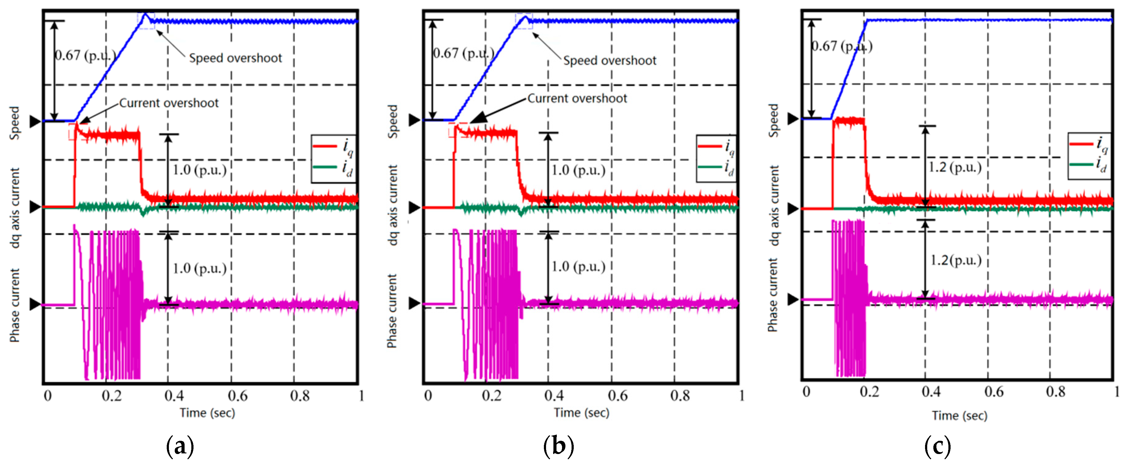
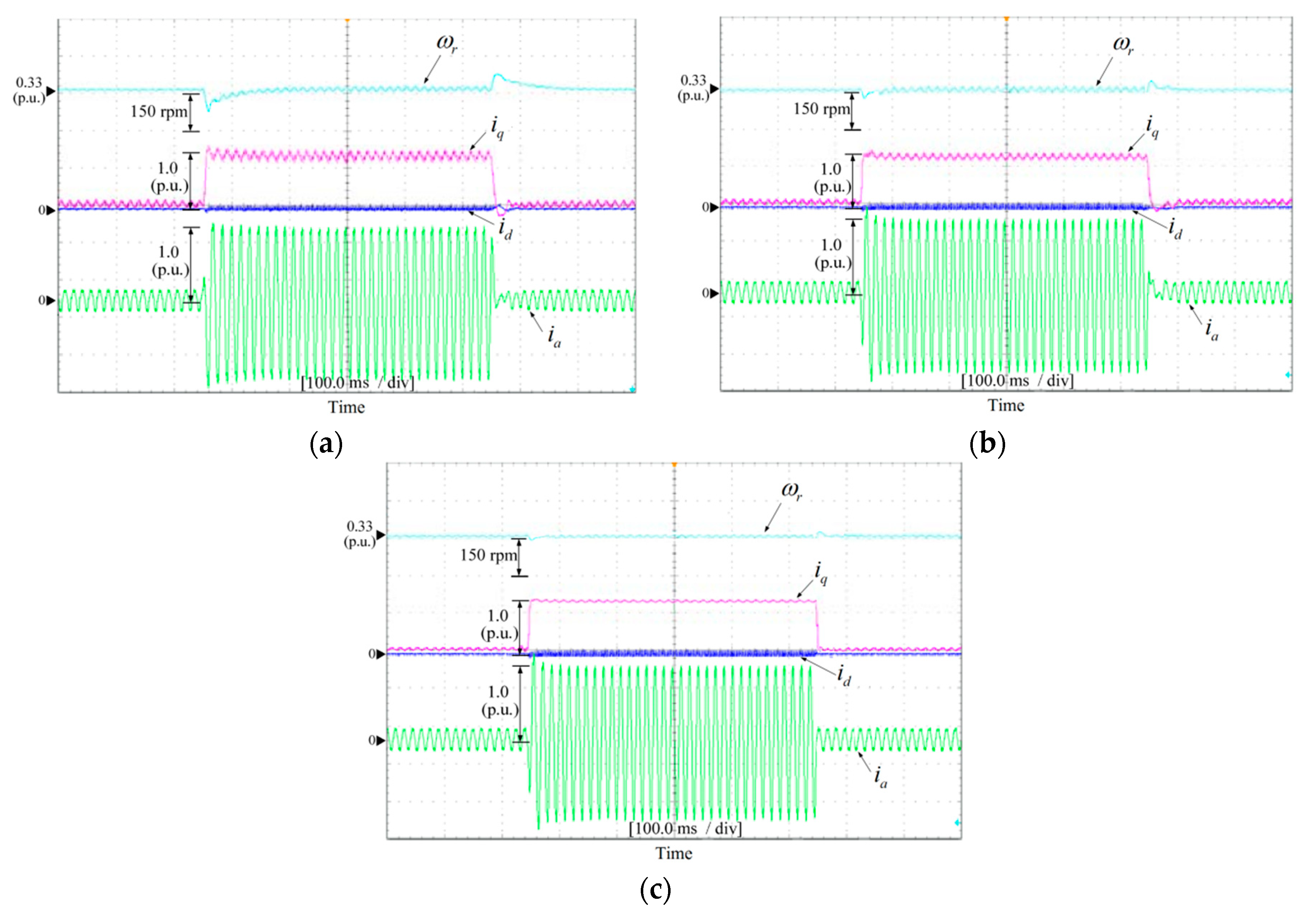
4.1.1. Comparison during Startup

Figure 3 gives the dynamic performance of motor starting with appropriate parameters under no-load condition, which include the motor speed, dq axis current and phase current. In the figure, all waveforms are denoted according to the rated value. The motor is given 0.67 times the rated speed to start. For the TBC, as in Figure 3a, it takes about 200 ms for the motor to reach the given value, and the speed overshoot is about 20 rpm. At the moment of motor starting, there is about 15% overregulation of rated current in the torque current. Figure 3b shows the performance of the AIBC_FP, and the speed adjustment time is almost the same as the TBC. The speed overshoot is reduced to 10 rpm and torque current overshoot is reduced to 10% rated current. For the AIBC_AWPSO, as in Figure 3c, the speed adjustment time is reduced to about 100 ms, and there is almost no overshoot in speed and torque current. Comparing Figure 3a, Figure 3b and Figure 3c, in terms of speed regulation time, the TBC is the same as the AIBC_FP, and the AIBC_AWPSO performance was better than the TBC and the AIBC_FP. In terms of the speed and current overshoot, the AIBC_AWPSO performs best, followed by the AIBC_FP, and the worst was the TBC. In addition, the steady-state speed fluctuation of the AIBC_AWPSO is less than that of the TBC and the AIBC_FP. The comparison shows that the AIBC_AWPSO has better dynamic control performance than the AIBC_FP and the TBC.

4.1.2. Comparison with Mismatched Resistance

In this section, the robustness to resistance parameter perturbation of the TBC and the AIBC_FP are compared, and the simulation waveforms are shown in Figure 4. Figure 4a shows the simulation result when the resistance parameter in the TBC is equal to two times the rated value. In transient state, the feedback of q axis current is larger than the given value (1.0 p.u.). At this time, if the limit value is set large, it may lead to overcurrent of hardware system and damage IPM or switching devices. What’s worse, Figure 4a shows a 50% current static error between the q-axis current instruction and the actual value. For the AIBC_FP, as in Figure 4b, the resistance parameter in the AIBC_FP is equal to two times the rated value too, and the q-axis current feedback can accurately track the instruction without oscillation or static error.

4.1.3. Comparison with Mismatched Inductance

In this section, the mismatch between inductance parameter in the controller and the actual in the TBC and the AIBC_FP are simulated and compared to verify that the AIBC can effectively improve the robustness of the controller to inductance perturbation, and the simulation results are shown in Figure 5. Figure 5a shows the simulation result when the inductance in the TBC is set to 2.5 times the actual inductance. From the simulation result, it can be seen that the dq axis current and the phase current have obvious oscillation.

Figure 5b shows the simulation result when the inductance in the AIBC_FP is set to two times the actual inductance, and the simulation result show that even if the inductance in the controller deviates from the actual, the dq axis current and the phase current remain stable, and the transient and steady-state performance are still good, which verify that the AIBC can effectively improve the robustness of the controller to inductance perturbation.

4.1.4. Comparison under Load Sudden Change Condition

Figure 6 gives the simulation results under load sudden change condition. The motor runs steadily at 150 rpm. The rated load (2.39 N·m) is suddenly added at 0.4 s and unloaded at 0.7 s. It can be seen from the figure that the fluctuation of the TBC’s speed is about 68 rpm, the AIBC_FP’s is about 37 rpm while the AIBC_AWPSO’s is about only 15 rpm when the load changes suddenly. In addition, the fluctuation of the torque current decreases obviously from the TBC to the AIBC_AWPSO. Comparing Figure 6a, Figure 6b and Figure 6c, in terms of load disturbance resistance, the AIBC_AWPSO performs best, followed by the AIBC_FP, and the worst was the TBC, which verify that the AIBC and the AWPSO can effectively improve the load disturbance resistance of the controller.

Table 6. Performance comparison of three control methods.

Control Method	Comparison during Startup	Comparison with Mismatched Resistance	Comparison with Mismatched Inductance	Comparison under Load Sudden Change Condition
TBC	Rise time: 200 ms; Speed overshoot: 20 rpm; Current overshoot: 15% of rated current	50% current static error	Obvious current oscillation	Speed fluctuation: 68 rpm
AIBC_FP	Rise time: 200 ms; Speed overshoot: 10 rpm; Current overshoot: 10% of rated current	No current static error	No current oscillation	Speed fluctuation: 37 rpm
AIBC_AWPSO	Rise time: 100 ms; Speed overshoot: 0 rpm; Current overshoot: 0% of rated current			Speed fluctuation: 15 rpm

summarizes the performance comparison of three control methods above.

4.2. Experimental Results

To validate the effectiveness of the proposed control strategy, experimental tests were carried out on a 750w PMSM test bench. Motor parameters are the same as Table 5, and the experimental tests were carried out on the testbench as shown in Figure 7, which includes the controlled PMSM, PMSM controller, hysteresis dynamometer, and control display instrument. The load torque of the controlled PMSM is given by the dynamometer controller to simulate the external load disturbance. In the experimental tests, the developed control algorithm is implemented on a 32-bit floating point DSP TMS320F28335, and the actual speed of the rotor are detected by an absolute encoder.

4.2.1. Comparison during Startup

Figure 8 shows the experimental results of motor starting with appropriate parameters under no-load condition. The experimental condition is consistent with Figure 3. It can be seen from the figure that besides the AIBC_AWPSO, there are obvious overshoot of speed and torque current in the TBC and the AIBC_FP control system. And the speed regulation time of the AIBC_AWPSO is much shorter than that of the TBC and the AIBC_FP (the motor can accelerate to 2000 rpm in about 150 ms without overshoot in the AIBC_AWPSO control system), which shows that the AIBC_AWPSO has better dynamic control performance than the TBC and the AIBC_FP. Therefore, we can consider applying the AIBC_AWPSO to the occasion where the dynamic requirements of motor speed are high (e.g., the motor needs rapid acceleration and deceleration).

4.2.2. Comparison with Mismatched Resistance

Figure 9 is the experimental comparison of the robustness to resistance parameter perturbation between the TBC and the AIBC_FP. Figure 9a is the experimental waveform of the TBC when the resistance parameter in the controller is equal to two times the rated value. The feedback of torque current is greater than the current instruction in transient state, which exceeds the current limit. This is consistent with the phenomenon in the simulation of Figure 4a. Figure 9b is the experimental waveform of the AIBC_FP when the resistance parameter is equal to two times the rated value. It can be seen that the current control performance is good. Whether in transient or steady state, current feedback can strictly track the current instruction.

4.2.3. Comparison with Mismatched Inductance

Figure 10 is an experimental comparison of the robustness to inductance parameter perturbation between the TBC and the AIBC_FP. Figure 10a is the experimental waveform of the TBC when the inductance parameter in the controller is equal to two times the rated value. From the experimental waveform, it can be seen that the dq axis current and phase current oscillation is obvious, and the current control performance is poor. Figure 10b is the experimental waveform of the AIBC_FP when the inductance parameter in the controller is equal to two times the rated value. From the experimental waveform, it can be seen that even if there is a big deviation between inductance in the controller and rated value in AIBC_FP, the system can maintain good current control performance, and the dq axis current and phase current are stable. The experimental result is in agreement with the simulation result (Figure 5b). It is proved that the AIBC can effectively compensate the current error caused by inductance mismatch. The robustness of the system to inductance parameter perturbation is improved, and the scope of application of inductance parameter is expanded. The transient and steady state performance of the system is maintained while the stability of the system is guaranteed.

4.2.4. Comparison under Load Sudden Change Condition

Figure 11 is the experimental waveform under abrupt load change. During the experiment, the rated load is suddenly loaded and unloaded by dynamometer, and the motor runs steadily at 150 rpm. Comparing Figure 11a, Figure 11b and Figure 11c, it can be seen that the speed and torque current of the TBC and the AIBC_FP system fluctuate significantly at the moment of sudden load change (the TBC is more obvious than the AIBC_FP, the TBC fluctuates about 75 rpm, while the AIBC_FP only reaches about 30 rpm), while the AIBC_AWPSO system has almost no speed and current fluctuation.

In addition, the vibration of the speed and torque current of the TBC and the AIBC_FP system is more obvious than that of no-load condition after adding the rated load, while the AIBC_AWPSO system has no obvious change compared with no-load condition. This proves that the AIBC_AWPSO system has strong resistance to external load disturbance.

5. Conclusions

This article present an AIBC for PMSMs with AWPSO parameter optimization, which effectively suppress the influence of load torque disturbance and inductance uncertainties of the dq axis on the system, and the parameters tuning problem of the controller is effectively solved. The integral terms of dq axis current following error are introduced into the control law, and the adaptive law with the differential term and the control law with the integral terms of the current error are derived to weaken the influence of internal parameters perturbation on current control. The AWPSO algorithm is used to optimize the parameters of the AIBC. Aiming at the parameters tuning problem of AIBC with differential term, a method for transforming multi-objective optimization with convex Prato frontier into single-objective optimization is presented. By this method, a form of fitness function suitable for parameters optimization of backstepping controller is determined, and according to the theoretical derivation and large number of simulation results, the corresponding parameters of the optimization algorithm are set. By randomly adjusting the inertia weight and changing the acceleration factor, the algorithm can accelerate the convergence speed and solve the problem of parameters optimization of AIBC.

The simulation and experiment compare the TBC, the AIBC_FP and the AIBC_AWPSO, which include the dynamic performance of motor starting, the robustness of control system to internal parameters perturbation under mismatch of resistance and inductance, and the robustness to external load perturbation under sudden loading and unloading of rated load. The simulation and experimental results show that the AIBC_AWPSO performs best, followed by the AIBC_FP, and the worst is the TBC in consideration of the dynamic performance of the system during motor starting. The TBC has no robustness to stator resistance and inductance perturbation, and current control under mismatch of resistance and inductance produces static error and vibration. The AIBC_FP has strong robustness to internal parameters perturbation. The AIBC_AWPSO also performs best in resisting external load disturbance, followed by the AIBC_FP and the TBC.

References

1. Onsal, M.; Cumhur, B.; Demir, Y.; Yolacan, E. Rotor Design Optimization of a New Flux-Assisted Consequent Pole Spoke-Type Permanent Magnet Torque Motor for Low-Speed Applications. IEEE Trans. Magn. 2018, 54, 1–5. [Google Scholar] [CrossRef]
2. Yolacan, E.; Guven, M.K.; Aydin, M. A Novel Torque Quality Improvement of an Asymmetric Windings Permanent-Magnet Synchronous Motor. IEEE Trans. Magn. 2017, 53, 1–6. [Google Scholar] [CrossRef]
3. Wang, Z.; Chen, J.; Cheng, M.; Chau, K.T. Field-Oriented Control and Direct Torque Control for Paralleled VSIs Fed PMSM Drives With Variable Switching Frequencies. IEEE Trans. Power Electron. 2016, 31, 2417–2428. [Google Scholar] [CrossRef]
4. Liang, D.; Li, J.; Qu, R.; Kong, W. Adaptive Second-Order Sliding-Mode Observer for PMSM Sensorless Control Considering VSI Nonlinearity. IEEE Trans. Power Electron. 2018, 33, 8994–9004. [Google Scholar] [CrossRef]
5. Rachid, E.; Ahmed, J.D.; Muyeen, S.M. Experimental Validation of a Novel PI Speed Controller for AC Motor Drives With Improved Transient Performances. IEEE Trans. Control Syst. Tech. 2018, 26, 1414–1421. [Google Scholar]
6. Tursini, M.; Parasiliti, F.; Zhang, D. Real-time gain tuning of PI controllers for high-performance PMSM drives. IEEE Trans. Ind. Appl. 2002, 38, 1018–1026. [Google Scholar] [CrossRef]
7. Liu, J.; Li, H.; Deng, Y. Torque Ripple Minimization of PMSM Based on Robust ILC Via Adaptive Sliding Mode Control. IEEE Trans. Power Electron. 2018, 33, 3655–3671. [Google Scholar] [CrossRef]
8. Zhang, X.; Sun, L.; Zhao, K.; Sun, L. Nonlinear Speed Control for PMSM System Using Sliding-Mode Control and Disturbance Compensation Techniques. IEEE Trans. Power Electron. 2013, 28, 1358–1365. [Google Scholar] [CrossRef]
9. Liu, X.; Yu, H.; Yu, J.; Zhao, L. Combined Speed and Current Terminal Sliding Mode Control With Nonlinear Disturbance Observer for PMSM Drive. IEEE Access. 2018, 6, 29594–29601. [Google Scholar] [CrossRef]
10. Víctor, R.; Domingo, B.; Antoni, A. Fixed Switching Period Discrete-Time Sliding Mode Current Control of a PMSM. IEEE Trans. Ind. Electron. 2018, 65, 2039–2048. [Google Scholar]
11. Tomasz, T.; Lech, M.G. Constrained State Feedback Speed Control of PMSM Based on Model Predictive Approach. IEEE Trans. Ind. Electron. 2016, 63, 3867–3875. [Google Scholar]
12. Farhad, A. Optimal Feedback Linearization Control of Interior PM Synchronous Motors Subject to Time-Varying Operation Conditions Minimizing Power Loss. IEEE Trans. Ind. Electron. 2018, 65, 5414–5421. [Google Scholar]
13. Choi, Y.S.; Choi, H.H.; Jung, J.W.; Kong, W. Feedback Linearization Direct Torque Control With Reduced Torque and Flux Ripples for IPMSM Drives. IEEE Trans. Power Electron. 2016, 31, 3728–3737. [Google Scholar] [CrossRef]
14. Li, J.; Ren, H.; Zhong, Y.; Kong, W. Robust Speed Control of Induction Motor Drives Using First-Order Auto-Disturbance Rejection Controllers. IEEE Trans. Ind. Appl. 2015, 51, 712–720. [Google Scholar] [CrossRef]
15. Zuo, Y.; Zhu, X.; Quan, L.; Zhang, C. Active Disturbance Rejection Controller for Speed Control of Electrical Drives Using Phase-Locking Loop Observer. IEEE Trans. Ind. Electron. 2018, 66, 1748–1759. [Google Scholar] [CrossRef]
16. Yin, Z.; Du, C.; Liu, J.; Sun, X. Research on Autodisturbance-Rejection Control of Induction Motors Based on an Ant Colony Optimization Algorithm. IEEE Trans. Ind. Electron. 2018, 65, 3077–3094. [Google Scholar] [CrossRef]
17. Wang, G.; Liu, R.; Zhao, N.; Ding, D. Enhanced Linear ADRC Strategy for HF Pulse Voltage Signal Injection-Based Sensorless IPMSM Drives. IEEE Trans. Power Electron. 2019, 34, 514–525. [Google Scholar] [CrossRef]
18. Marcin, M. The Adaptive Backstepping Control of Permanent Magnet Synchronous Motor Supplied by Current Source Inverter. IEEE Trans. Ind. Inform. 2013, 9, 1047–1055. [Google Scholar]
19. Jesús, L.F.; Carlos, G.R.; Hebertt, S.R.; Oscar, D. Robust Backstepping Tracking Controller for Low-Speed PMSM Positioning System: Design, Analysis, and Implementation. IEEE Trans. Ind. Inform. 2015, 11, 1130–1141. [Google Scholar]
20. Liu, S.; Guo, X.; Zhang, L. Robust Adaptive Backstepping Sliding Mode Control for Six-Phase Permanent Magnet Synchronous Motor Using Recurrent Wavelet Fuzzy Neural Network. IEEE Access. 2017, 5, 14502–14515. [Google Scholar]
21. Zhang, Y.; Wen, C.; Yeng, C. Discrete-time robust backstepping adaptive control for nonlinear time-varying systems. IEEE Trans. Autom. Control 2000, 45, 1749–1755. [Google Scholar] [CrossRef] [Green Version]
22. Sun, L.; Zheng, Z. Disturbance-Observer-Based Robust Backstepping Attitude Stabilization of Spacecraft Under Input Saturation and Measurement Uncertainty. IEEE Trans. Ind. Electron. 2017, 64, 7994–8002. [Google Scholar] [CrossRef]
23. Kokotovic, P.V. The joy of feedback: Nonlinear and adaptive. IEEE Control Syst. Mag. 1992, 12, 7–17. [Google Scholar]
24. Shieh, H.J.; Shyu, K.K. Nonlinear sliding-mode torque control with adaptive backstepping approach for induction motor drive. IEEE Trans. Ind. Electron. 1999, 46, 380–389. [Google Scholar] [CrossRef]
25. Ba, D.; Yeom, H.; Kim, J.; Bae, J. Gain-Adaptive Robust Backstepping Position Control of a BLDC Motor System. IEEE/ASME Trans. Mechatron. 2018, 23, 2470–2481. [Google Scholar]
26. Hsu, C.F.; Lin, C.M.; Lee, T.T. Wavelet Adaptive Backstepping Control for a Class of Nonlinear Systems. IEEE Trans. Neural Netw. 2006, 17, 1175–1183. [Google Scholar]
27. Yu, X.; Lin, Y. Adaptive Backstepping Quantized Control for a Class of Nonlinear Systems. IEEE Trans. Autom. Control 2017, 62, 981–985. [Google Scholar] [CrossRef]
28. Cai, J.; Wen, C.; Su, H.; Liu, Z. Adaptive Backstepping Control for a Class of Nonlinear Systems With Non-Triangular Structural Uncertainties. IEEE Trans. Autom. Control 2017, 62, 5220–5226. [Google Scholar] [CrossRef]
29. Sun, L.; Huo, W.; Jiao, Z. Adaptive Backstepping Control of Spacecraft Rendezvous and Proximity Operations With Input Saturation and Full-State Constraint. IEEE Trans. Ind. Electron. 2017, 64, 480–492. [Google Scholar] [CrossRef]
30. Lin, F.J.; Chang, C.K.; Huang, P.K. FPGA-Based Adaptive Backstepping Sliding-Mode Control for Linear Induction Motor Drive. IEEE Trans. Power Electron. 2007, 22, 1222–1231. [Google Scholar] [CrossRef]
31. Rahman, M.A.; Vilathgamuwa, D.M.; Uddin, M.N.; Tseng, K.J. Nonlinear control of interior permanent-magnet synchronous motor. IEEE Trans. Ind. Appl. 2003, 39, 408–416. [Google Scholar] [CrossRef]
32. Chen, M.; Lu, S.; Tseng, K.J. Application of Adaptive Variable Speed Back-Stepping Sliding Mode Controller for PMLSM Position Control. J. Mar. Sci. Technol. 2014, 22, 392–403. [Google Scholar]
33. Kim, S.K.; Lee, K.G.; Lee, K.B. Singularity-Free Adaptive Speed Tracking Control for Uncertain Permanent Magnet Synchronous Motor. IEEE Trans. Power Electron. 2016, 31, 1692–1701. [Google Scholar] [CrossRef]
34. Sarikhani, A.; Nejadpak, A.; Mohammed, O.A. Coupled Field-Circuit Estimation of Operational Inductance in PM Synchronous Machines by a Real-Time Physics-Based Inductance Observer. IEEE Trans. Magn. 2013, 49, 2283–2286. [Google Scholar] [CrossRef]
35. Ni, R.; Wang, G.; Gui, X.; Xu, D. Investigation of d and q-Axis Inductances Influenced by Slot-Pole Combinations Based on Axial Flux Permanent-Magnet Machines. IEEE Trans. Ind. Electron. 2014, 61, 4539–4551. [Google Scholar] [CrossRef]
36. Lin, C.M.; Li, H.Y. Intelligent Control Using the Wavelet Fuzzy CMAC Backstepping Control System for Two-Axis Linear Piezoelectric Ceramic Motor Drive Systems. IEEE Trans. Fuzzy Syst. 2014, 22, 791–802. [Google Scholar] [CrossRef]
37. Chaoui, H.; Sicard, P. Adaptive Fuzzy Logic Control of Permanent Magnet Synchronous Machines With Nonlinear Friction. IEEE Trans. Ind. Electron. 2012, 59, 1123–1133. [Google Scholar] [CrossRef]
38. Kung, Y.S.; Tsai, M.H. FPGA-Based Speed Control IC for PMSM Drive With Adaptive Fuzzy Control. IEEE Trans. Power Electron. 2007, 22, 2476–2486. [Google Scholar] [CrossRef]
39. Barkat, S.; Tlemcani, A.; Nouri, H. Noninteracting Adaptive Control of PMSM Using Interval Type-2 Fuzzy Logic Systems. IEEE Trans. Fuzzy Syst. 2011, 19, 925–936. [Google Scholar] [CrossRef]
40. Li, S.; Gu, H. Fuzzy Adaptive Internal Model Control Schemes for PMSM Speed-Regulation System. IEEE Trans. Ind. Inform. 2012, 8, 767–779. [Google Scholar] [CrossRef]
41. Mahfouf, M.; Chen, M.Y.; Linkens, D.A. Adaptive Weighted Particle Swarm Optimization for Multi-objective Optimal Design of Alloy Steelss. In Proceedings of the 8th International Conference Parallel Problem Solving from Nature, Birmingham, UK, 18–22 September 2004; Volume 19, pp. 762–771. [Google Scholar]
42. Parikshit, Y.; Rajesh, K.; Panda, S.K.; Chang, C.S. An Intelligent Tuned Harmony Search Algorithm for Optimisation. Inform. Sci. 2012, 196, 47–72. [Google Scholar]
43. Li, J. Distributed cooperative tracking of multi-agent systems with actuator faults. Trans. Inst. Meas. Control. 2015, 37, 1041–1048. [Google Scholar] [CrossRef]
44. Li, J.; Li, C.; Yang, X.; Chen, W. Event-triggered containment control of multi-agent systems with high-order dynamics and input delay. Electronics 2018, 7, 343. [Google Scholar] [CrossRef]
45. Du, Z.; Zhang, Q.; Liu, L. New delay-dependentrobust stability of discrete singular systems with time-varying delay. Asian Journal of Control. 2011, 13, 136–147. [Google Scholar] [CrossRef]
46. Wei, C.; Hao, L.; Yang, T.; Liu, J. Trajectory Optimization of Electrostatic Spray Painting Robots on Curved Surface. Coatings 2017, 7, 155. [Google Scholar] [CrossRef]
Figure 1. Structure of the anti-saturation torque observer.
Energies 12 02596 g001
Figure 2. Flowchart of AWPSO.
Energies 12 02596 g002
Figure 3. Simulation results of motor starting with appropriate parameters under no-load condition: (a) TBC; (b) AIBC_FP; (c) AIBC_AWPSO.
Energies 12 02596 g003
Figure 4. Simulation results of motor starting with mismatched resistance: (a) TBC; (b) AIBC_FP.
Energies 12 02596 g004
Figure 5. Simulation results of motor starting with mismatched inductance: (a) TBC; (b) AIBC_FP.
Energies 12 02596 g005
Figure 6. Simulation results under load sudden change condition: (a) TBC; (b) AIBC_FP; (c) AIBC_AWPSO.
Energies 12 02596 g006
Figure 7. The testbench for PMSM drive system.
Energies 12 02596 g007
Figure 8. Experimental results of motor starting with appropriate parameters under no-load condition: (a) TBC; (b) AIBC_FP; (c) AIBC_AWPSO.
Energies 12 02596 g008
Figure 9. Experimental results of motor starting with mismatched resistance: (a) TBC; (b) AIBC_FP.
Energies 12 02596 g009
Figure 10. Experimental results of motor starting with mismatched inductance: (a) TBC; (b) AIBC_FP.
Energies 12 02596 g010
Figure 11. Simulation results under load sudden change condition: (a) TBC; (b) AIBC_FP; (c) AIBC_AWPSO.
Energies 12 02596 g011