CFD Computation of the H-Darrieus Wind Turbine—The Impact of the Rotating Shaft on the Rotor Performance

Abstract

Aerodynamics of the Darrieus wind turbine is an extremely complex issue requiring the use of very advanced numerical methods. Additional structural components of this device, such as, for example, a rotating shaft disturb the flow through the rotor significantly impairing its aerodynamic characteristics. The main purpose of the presented research is to validate the commonly-used unsteady Reynolds averaged Navier–Stokes (URANS) approach with the shear stress transport (SST) k-ω turbulence model based on the particle image velocimetry (PIV) studies of a two-bladed rotor operating at the moderate tip speed ratio of 4.5. In the present numerical studies, a two-dimensional turbine rotor with a diameter of 1 m was considered. The following parameters were evaluated: instantaneous velocity fields; velocity profiles in the rotor shadow and aerodynamic blade loads. The obtained numerical results are comparable with the reference experimental results taken from the literature. The second purpose of this work was to examine the influence of the rotating rotor shaft/tower on the wind turbine performance. It has been proven that the cylindrical shaft reduces the power of the device by 2.5% in comparison with the non-shaft configuration.

1. Introduction

Basically, the tower is an inseparable element of most types of wind turbines. In the case of horizontal-axis wind turbines (HAWTs), it may be located in front of the propeller, such turbines are called downwind HAWTs, or behind the propeller, upwind HAWTs. In the case of the Darrieus wind turbine, the shaft/tower is usually placed in its axis of rotation. The presence of the tower disrupts the flow around the rotor and thereby reduces the performance of all mentioned types of wind turbines. In the case of the upwind HAWTs, the tower stops the flow in front of it and thus reduces the air velocity on the blades passing in front of the tower. In the case of the downwind HAWTs and the Darrieus wind turbines, their blades pass through the tower shadow. In addition, the shaft of the Darrieus wind turbine rotates with the entire rotor which further complicates the flow. In the case of propeller-type wind turbines, many studies have been carried out regarding the influence of the tower on performance [1,2,3]. In the case of vertical-axis wind turbines, such investigations are definitely less.

The influence of the tower on the performance of the vertical-wind turbine is one of the so-called secondary effects. These effects result from the presence of spoilers, struts, rotating tower, airfoil type, and so on. In general, with the increase of the tip speed ratio, the impact of the secondary effects is larger. The tip speed ratio is called the ratio of blade velocity to the wind speed. Each blade of the Darrieus wind turbine extracts energy from the wind passing through the upwind as well as the downwind side of the rotor. In the case of smaller tip speed ratios, the rotor blade moves more slowly than the main flow, thus it disturbs the flow less. In the case of larger tip speed ratios, the blade moves faster than the undisturbed flow, which causes larger disturbances of the main flow, especially in the downwind part of the rotor which results in decreasing its aerodynamic performance. Additional structural elements of the rotor, such as struts or rotating tower, further reduce the rotor performance, especially in its downwind part. According to I. Paraschivoiu [4], the presence of the tower reduces the tangential force in both the upwind and downwind side of the rotor. This is because the flow in front of the tower is slowed down and the aerodynamic wake behind it is disturbed.

The double-multiple streamtube (DMS) method, based on the conservation of momentum principle in a quasi-steady flow, the tower effect is taken into account based on Glauert’s theory. The presence of the tower in the flow is modeled by assuming a uniform velocity deficit into the streamtube. This velocity deficit is calculated on the basis of the tower drag coefficient. In this classical theory, the aerodynamic wake behind the rotor has a Gaussian distribution whereas the flow in the wake is considered as a disturbance that is linearly superposed on the main flow [4,5]. Paraschivoiu et al. [6] were among the first who applied this theory into the double-multiple streamtube model. These authors studied the aerodynamic performance of two wind turbines the Sandia 5-m at 175 rpm (the ratio of the tower diameter to the maximum rotor diameter was 0.035) and the Sandia 17-m at 50.6 rpm, employing the DMS model with variable interference factor (the velocity on the rotor was dependent on the azimuth). For the smaller rotor having the tower, the authors obtained the maximum power coefficient less by 2% compared to the clean rotor. Similarly, in the case of the Sandia 17-m, the difference in maximum power coefficient obtained using the tested model and experimental values was almost imperceptible. For this reason, the effect of the tower was and still is neglected very often in calculations [7,8].

Klimas [9] showed a more advanced approach, vortex Darrieus turbine (VDART) model, based on a vortex filament representation of the wind turbine blades as well as their aerodynamics wakes, for the analysis of the impact of the tower shadow on the performance characteristics of the 17-m rotor (the ratio of the rotor blade and radius chord, c/R, was 0.05). According to the predictions of the 2D version of this model, the rotor power coefficient drops almost linearly with the increase in the ratio of the tower radius, r₀, to the rotor radius, R, from 1.5% for r₀/R=0.04 to 4.7% for r₀/R=0.16 in comparison with the rotor without tower.

Today, the efforts of many researchers focus on the use of computational fluid dynamics (CFD) considering the unsteady Reynolds-averaged Navier–Stokes (URANS) equations for the analysis of aerodynamic properties of vertical-axis wind turbines. These methods are helpful, among other things, in the study of the dynamic stall phenomena occurring at low tip speed ratios, which results in enormous fluctuations in torque and power reduction [10]. Due to the fact that the URANS approach requires turbulence modeling, many authors compare the obtained numerical results using various turbulence models [11,12,13,14,15]. Momentum based aerodynamic models, such as the DMS model, fail in the case of rotors with a large rotor solidity, σ. This parameter depends on the number of blades, N, the blade chord length, c, and the rotor diameter, D: σ=Nc/D. Due to the large flow disturbance in the vicinity of rotors with a large solidity, CFD methods are an indispensable analytical tool in the process of optimizing the construction, much cheaper than experimental tests [16,17,18]. Small-scale vertical-axis wind turbines usually have a larger solidity due to the small rotor diameters. In such cases, three-dimensional flow effects can play an important role in prediction of flow detachment and significant reduction of rotor performance [19]. Earlier studies of the author of this paper, [20] or [21], as well as studies of other researchers—for example, [22] or [23]—confirm the high accuracy of the URANS technique as well as the SST turbulence model for high-solidity rotors, even for σ of 0.3. In some of these investigations, the rotor shaft was taken into account, but it was not the main topic of the research.

According to Rezaeiha et al. [24], the impact of the tower shadow of a small-scale wind turbine on the rotor performance is different than in the case of the large-scale wind turbines. Large aerodynamic drag of the shaft can affect the drag of the entire rotor and generate power losses. These authors analyzed the shaft-to-turbine diameter, δ, in the range from 0 to 16% for a rotor operating in the range of different tip speed ratio by utilizing URANS approaches. It has been proven that the power losses increase asymptotically as the shaft-to-turbine diameter increases up to 5.5% for δ=16% compared to a rotor without a shaft. The numerical results of Zhang et al. [25] shows that for δ of 9% the power loss of the rotor increases even up to 25% relative to the no-shaft rotor.

The purpose of this article is to determine the suitability of the commercial aerodynamic model, k-ω SST, for testing the aerodynamic blade loads of the rotor equipped with a shaft and without a shaft (clean rotor). An effort was made to examine the aerodynamic wake downstream behind the rotor and determine its effect on the loss of the tangential force. Validation of the model was carried out using experimental studies carried out using the particle image velocimetry (PIV) technique [26,27].

2. Characteristics of the VAWT

2.1. Vertical Axis Wind Turbine Concept and Aerodynamic Characteristics

A wind turbine with a vertical axis of rotation (vertical-axis wind turbine—VAWT) consists of several curved or straight blades that drive the generator shaft. By using the lift force to generate the torque, the tangential velocity of the blades can be larger compared to the wind speed. The silhouette of a wind turbine with straight blades (H-type rotor) is shown in Figure 1a. The rotor shown in this drawing has additional elements that attach the blades to the shaft and transfer the torque to the rotor shaft. These elements are called struts and they are usually profiled using symmetrical airfoils to minimize additional aerodynamic drag. In the case of the rotor investigated in this work, its blades also have symmetrical airfoils NACA0018. A lot of commercial wind turbines have symmetrical airfoils; they provide high efficiency in the upwind part of the rotor.

From the point of view of the commercial use of different types of wind turbines, two aspects are important: aerodynamic forces acting on the rotor blades and aerodynamic wake downstream behind the rotor. In particular, the tangential force, F_T, is responsible for creating the torque, that is also for the power generated by a given rotor. This aerodynamic force component as well as the normal force, F_N, depend on the position of the rotor, which uniquely defines the azimuth angle θ (Figure 1b). These forces are defined in this work as coefficients

$$c_{n,t}=F_{N,T}/R·q_0$$

(1)

where

$$q_0=\frac{1}{2}{V}_0^2·R·q$$

(2)

where V₀ is the undisturbed flow velocity; R is the rotor radius; q is the air density.

The flow field downstream behind the rotor is characterized by the wake velocity distribution. In this work, two components of the velocity field were analyzed: the component of velocity parallel to the wind direction, U_x, and the perpendicular component, U_y.

2.2. Method

The choice of the calculation method depends, among other things, on the flow parameters around the operating rotor. For the wind turbine rotor investigated in this work that operates at the tip speed ratio of 4.5, the flow velocity around the rotor blades is lower than 50 m/s which in a consequence gives the Mach number of 0.14 and therefore, the flow can be considered as an incompressible flow. Since the pulsations of aerodynamic forces are large, the flow cannot be considered as steady-state and therefore unsteady Reynolds-averaged Navier–Stokes governing equations must be employed.

The Menter’s Shear Stress Transport (SST) k-ω turbulence model, introduced in 1994 by F.R. Menter, was used in this work. This two-equation eddy-viscosity model combines two turbulence approaches: the standard k-ω model in the inner region of the boundary layer and the k-ε formulation in the free shear flow. The SST k-ω turbulence model is based on the assumption of Bradshaw that the principal shear stress is proportional to the kinetic energy of turbulence. A large number of different flow fields confirmed good agreement of the results obtained by this turbulence model with the experimental data [28].

In the research presented in this paper, the URANS approach implemented in commercial CFD software ANSYS Fluent was utilized. In the pressure-based solver that was used in these simulations, the constraint of mass conservation of the velocity field is obtained by solving the pressure equation. In the presented simulations, the segregated algorithm SIMPLEC was utilized for the pressure–velocity coupling. For the analyzed case, this method ensures quick convergence for the defined time step size. Moreover, the second-order discretization schemes were considered for pressure, momentum, and turbulent quantities. A time-accurate unsteady solution of the flow field around a rotating vertical-axis wind turbine was obtained using the sliding mesh model. This approach is often used when the unsteady interaction of the flow between stationary and moving grids has to be taken into account. The use of the sliding mesh model for simulation of the Darrieus wind turbine entails the creation of an additional moving computational domain that will move during the computational process. The convergence criteria for all calculated quantities were set to 10^-5. The underrelaxation factors for the turbulent kinetic energy, specific dissipation rate, and turbulent viscosity were set to 0.8, 0.8, and 1, respectively [29,30].

3. Wind Turbine and Computational Model

3.1. Experimental Test Case

In this work, the results of experimental studies by Tescione et al. [26] and Castelein et al. [27] were used to validate the numerical model. In these tests, the two-bladed H-type rotor was analyzed, operating at the tip speed ratio of 4.5. The velocity field was measured utilizing the phase-locked particle image velocimetry technique. Aerodynamic blade loads were determined on the basis of velocity field measurements. The PIV experiments were conducted in the Open Jet wind tunnel of TU Delft. The close-circuit wind tunnel has a 13.7 x 6.6 x 8.2 m test section. The free stream velocity is in the range from 3 to 34 m/s, whereas the turbulence level is 0.24%.

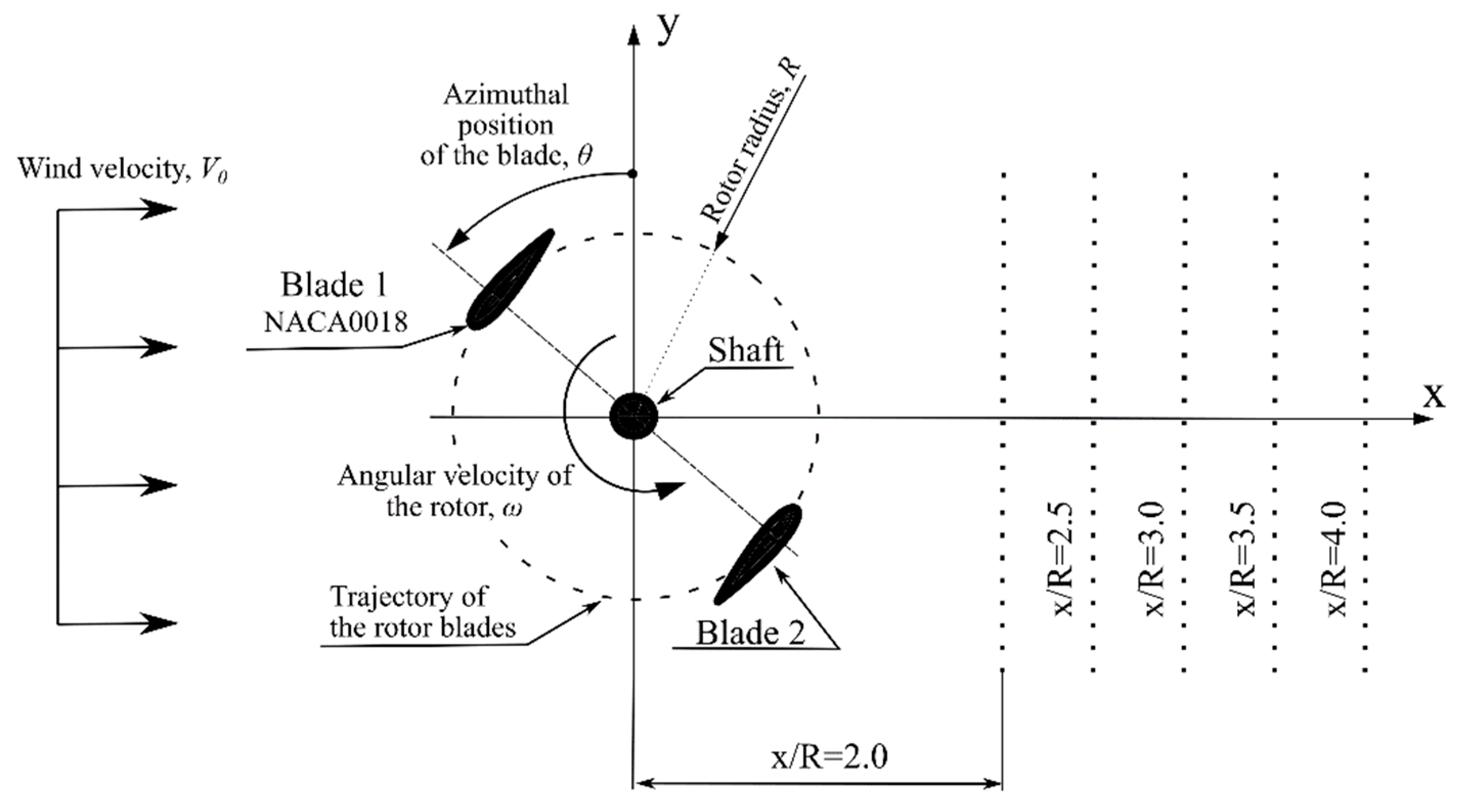
3.2. Wind Turbine Overview

In this work, a two-dimensional wind turbine rotor model was developed, consisting of two NACA 0018 airfoils and a rotor shaft. The investigated model is obviously simplified, the finite blade length and the presence of struts that fix the rotor blades to the rotor shaft were neglected in these studies. Basic geometrical parameters of the investigated wind turbine are introduced in

Table 1. Design specifications of the analyzed wind turbine.

Parameter	Value
Number of blades, N	2
Rotor diameter, D=2R	1 m
Chord length, c	0.06 m
Solidity, Nc/R	0.24
Blade airfoil	NACA0018
Rotor shaft diameter, DS	0.04 m

.

Numerical experiments have been performed for one tip speed ratio of 4.5. The rotor rotational velocity was 800 rpm and the free stream velocity, V₀, was 9.3 m/s. For given rotor operating conditions and for geometric parameters, the Reynolds number of the blade was 170,000. The conceptual model of the tested rotor is shown in Figure 2. This figure also shows the positions of the measuring points behind the rotor in which the velocity was collected. Other geometrical dimensions of the rotor are shown in Figure 3.

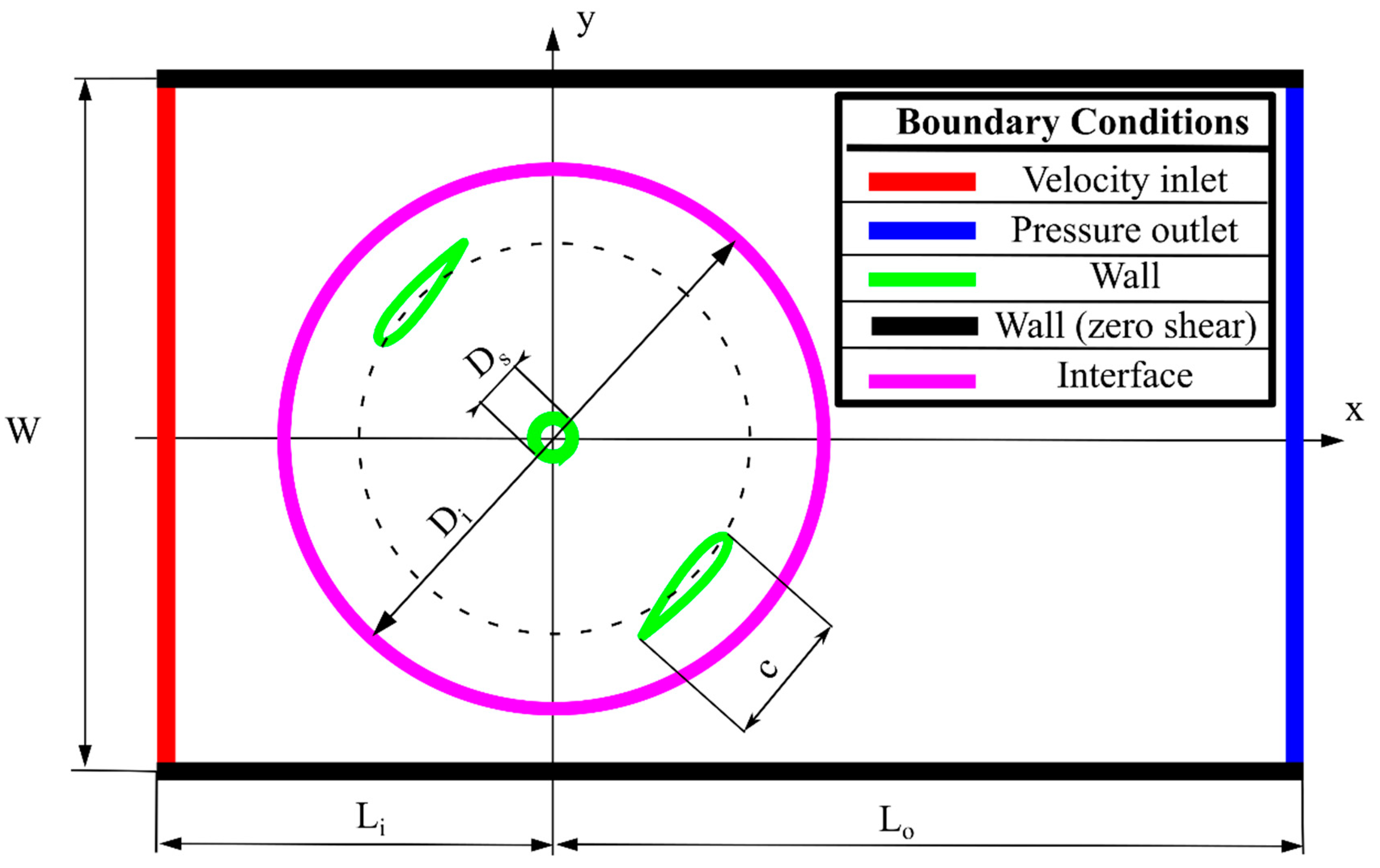
3.3. Computational Domain and Boundary Conditions

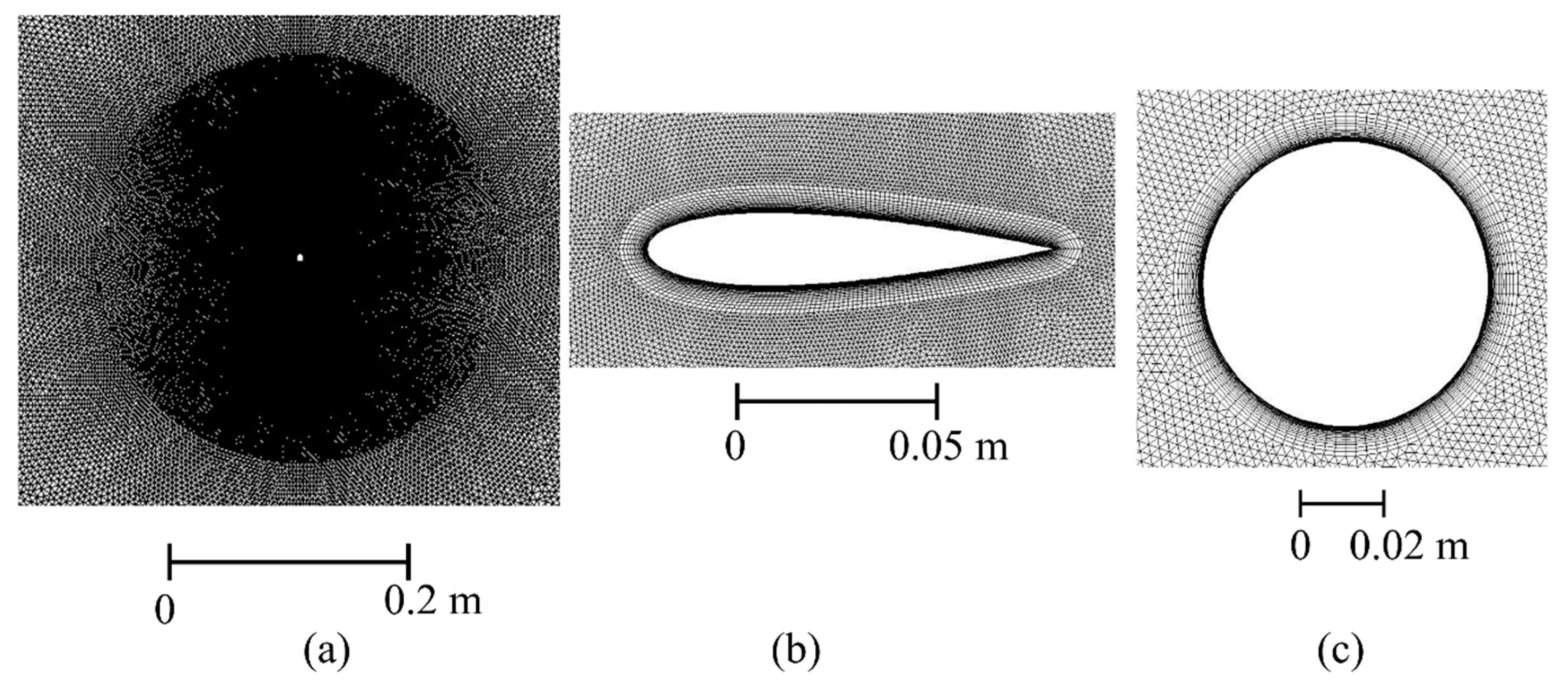
The rotor of a wind turbine consisted of blades and a shaft is surrounded by a rectangular area—a computing domain whose width corresponds to the width of the wind tunnel, W=6.6 m. Because the transient flow was considered, the sliding mesh technique was utilized. Using this technique requires specifying an additional area that will move along with the examined object during simulation. In these studies, a surface with a diameter of D_i = 2 m was created that surrounded the rotor. During simulation, data is transferred between areas via the interface. The remaining dimensions are assumed: distance between the rotor axis and the inlet, L_i = 6 m, and distance between the rotor axis and the outlet, L_o = 14 m. The influence of the diameters D_i, L_i and L_o on the performance of the wind turbine has not been studied in this work. A non-slip wall boundary condition was applied at the airfoil and shaft edges. In order to model smooth side walls of the wind tunnel a slip-wall boundary condition is used by specifying zero shear stress. The dimensions of the computational domain and boundary conditions are shown in Figure 3.

3.4. Mesh

The computational domain described in Section 3.3 has been discretized using a finite volume grid. A hybrid computational mesh consisting of a structural grid at the edges of the airfoils and the rotor shaft as well as a non-structural mesh in the remaining area was generated. Figure 4 shows the distribution of grid elements in the rotor area as well as in the vicinity of the airfoil and the shaft (Figure 4). The structured grid near the blade edges consists of 40 layers. The height of the first layer of is 10^-3 mm and the growth rate of subsequent structural grid layers is 1.18. Such thickness of the first layer of the structural grid provides an average value of the dimensionless parameter called wall y⁺ equal to 0.2. To ensure the best accuracy of flow parameters in the area of the rotor and behind it, the growth of unstructured grid elements was very small equal to 1.02. The number of uniform blade edge divisions is 200 and the shaft is 100. The total number of cells for the reference computing grid is 261,398. Section 4.5 presents the effect of grid density on aerodynamic blade loads calculated.

4. Results

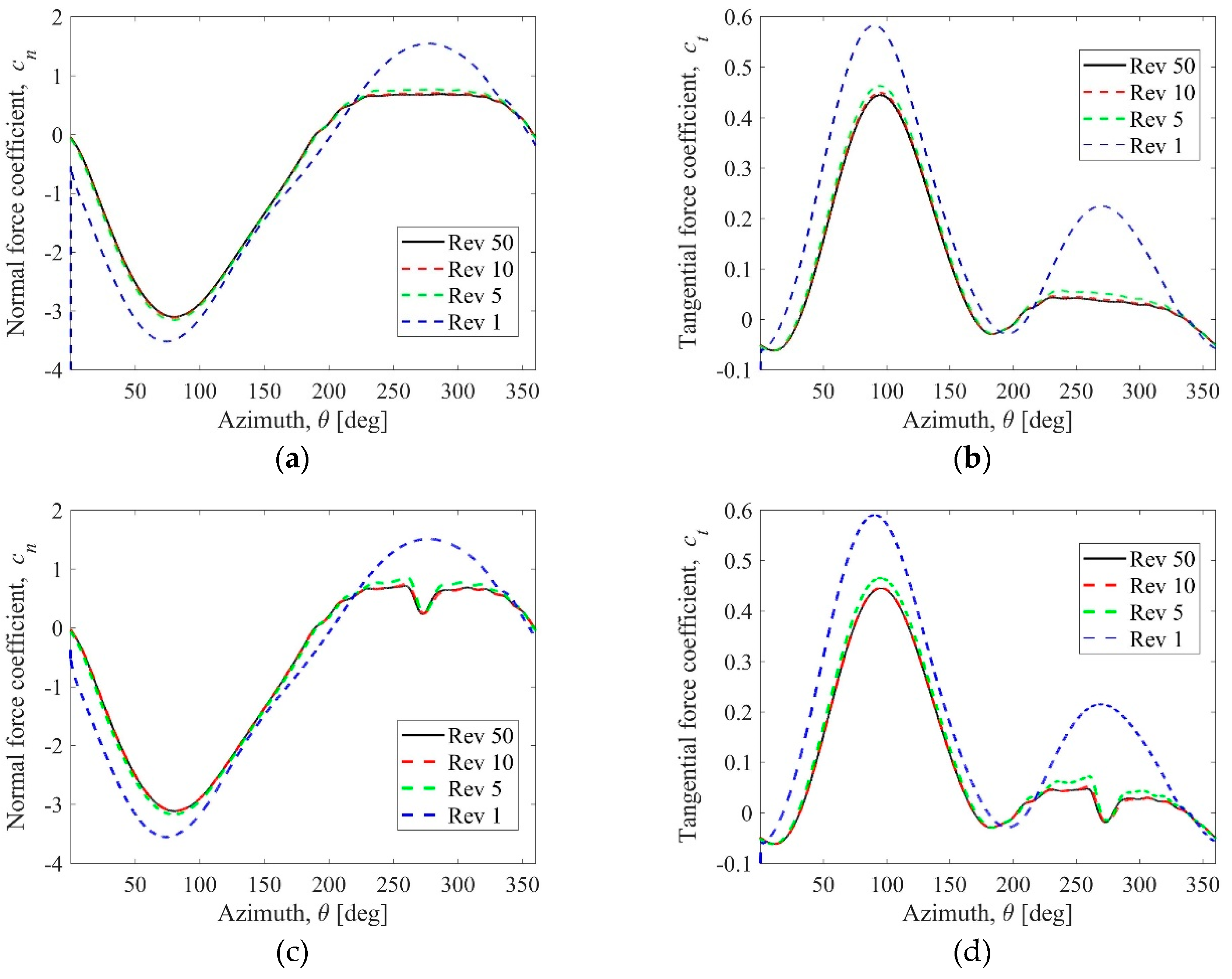
4.1. Aerodynamic Blade Loads

Figure 5a,b show two components of the aerodynamic force, normal and tangential respectively. The results are presented for the rotor consisting of two blades and for the rotor equipped with blades and a shaft. Only the results of the normal force component were compared to the experiment. The maximum value of the tangent component is seven times smaller in relation to the normal component. This creates enormous measurement problems, especially in the case of high tip speed ratios. Already in the 1970s and 1980s, this problem was reported, among others, by Strickland et al. [31] or Lanevile and Vittecoq [32]. The characteristics presented in the figures show an interesting effect, namely the influence of the shaft shadow is visible only in the vicinity of the azimuth angle θ=273 (deg). Aerodynamic characteristics for the upwind part of the rotor are almost identical; in the downwind region they are also very similar, but with the exception of the azimuthal location indicated in the previous sentence. From the engineering point of view, the local decrease in this tangential force causes a small loss of the rotor power coefficient, C_P, from 0.411 to 0.401. The largest difference between numerical and experimental results was observed for the θ=130 (deg). The measurement error in this rotor position is also the largest. Numerical studies conducted by Rogowski et al. [33] with the use of a more advanced technique, Scale Adaptive Simulation (SAS), have shown that even for rotors operating in the range of optimal tip speed ratios, the effects typical for dynamic stall can be noticeable. They are, however, possible to detect by using more advanced techniques and using three-dimensional Navier–Stokes equations. Slightly higher results of the calculated normal force compared to the experimental results seem to be justified due to the fact that the analyzed model was two-dimensional, and the blade tip losses were not taken into account in this work. The influence of the rotating shaft in the experiment differs slightly from that obtained in the calculations. The normal force curve appears to be more flat in the downwind part of the rotor. The lack of a visible peak in the experimental curve of the normal force may result from 3D effects, which the two-dimensional numerical model did not include.

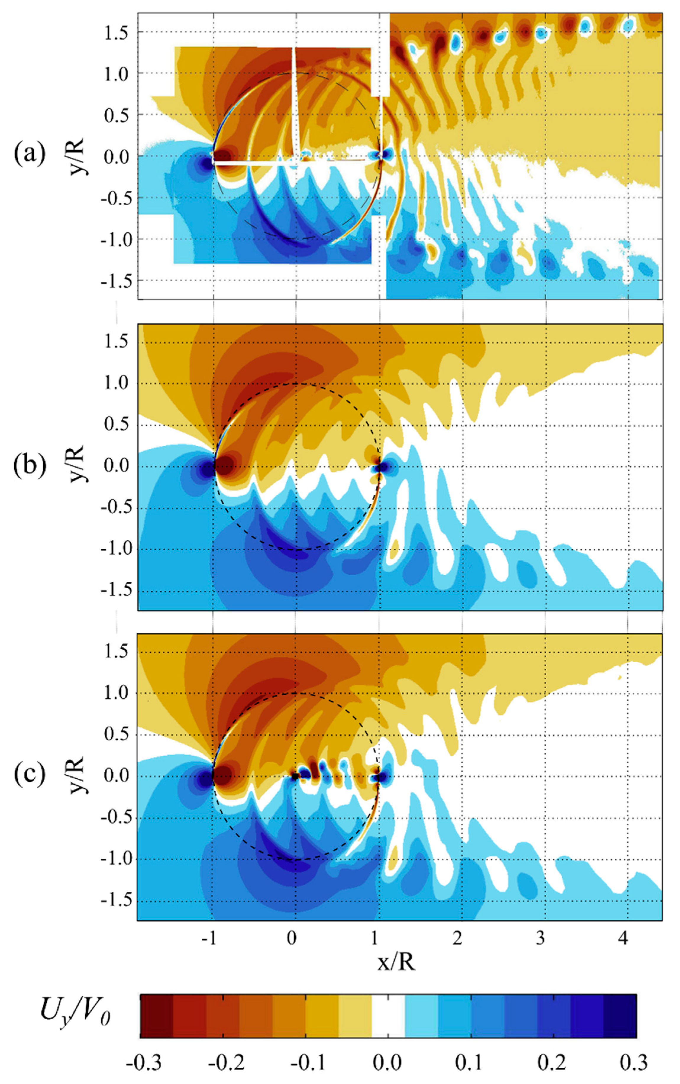
4.2. Aerodynamic Wake Characteristics

The presence of the rotor shaft does not cause only a local drop in tangential force, which was proved in the previous section. The flow structure in the downwind part of the rotor is also changed. In order to assess the aerodynamic wake behind the vertical-axis wind turbine rotor, a number of velocity measurements were made at certain distances downstream behind the rotor. The distances in which the velocity measurements were made are shown in Figure 2. Two velocity components were analyzed: parallel to wind direction, U_x, and perpendicular, U_y (Figure 1b). Figure 6 and Figure 7 present profiles of these velocity components averaged over the entire rotation of the rotor. The U_x,avr and U_y,avr symbols were used for the averaged values of these velocity components.

Velocity profiles U_x,avr calculated for both rotors differ slightly compared to experimental results (Figure 6). The differences are slightly lower in the case of the second velocity component, U_y,avr. These velocities are also related to wind speed, V₀. The shapes of the dominant velocity component calculated numerically resemble the Gaussian curve while the velocity profiles measured in the experiment are asymmetrical. In this work, the influence of struts on rotor performance has not been studied. The struts are in fact profiled beams fixing the blades to the shaft. Each rotor blade is attached to the shaft by means of two struts. The struts can change the flow structure downstream behind the rotor and cause asymmetry of velocity profiles. Another possible factor that affects the differences in the calculated and measured velocity profiles may be the turbulence model used (the SST k-ω model).

For y/R = 0.3 and x/R = 1.5, the influence of the shaft on the velocity profile is visible. With the increase in the ratio x/R, this effect gets smaller.

This paper also compares the computed instantaneous velocity distributions with the experimental results obtained with the PIV technique. Figure 8 shows contour maps of the velocity magnitude V normalized by the wind velocity V₀ for several azimuth positions of the same rotor blade. The numerical results were compared for the rotor with the shaft (Figure 8b) and the clean one (Figure 8a). The figure shows the effect of the shaft, which reduces the flow rate on the blade located in its shadow almost to zero.

Figure 9 shows the field of instantaneous velocity component U_x for one azimuth θ=90 deg while Figure 10 shows the distributions of the second component of the velocity field U_y for the same azimuthal position. The width of the aerodynamic wake downstream behind the rotor measured with the PIV technique is greater compared to the numerical results (Figure 9). In the case of the U_x velocity field, the shaft effect is also visible here (Figure 9c). In Figure 10, a larger area of zero velocity U_y is visible in comparison to the experiment. It seems that this drawing illustrates also other three-dimensional flow effects invisible in numerical simulations.

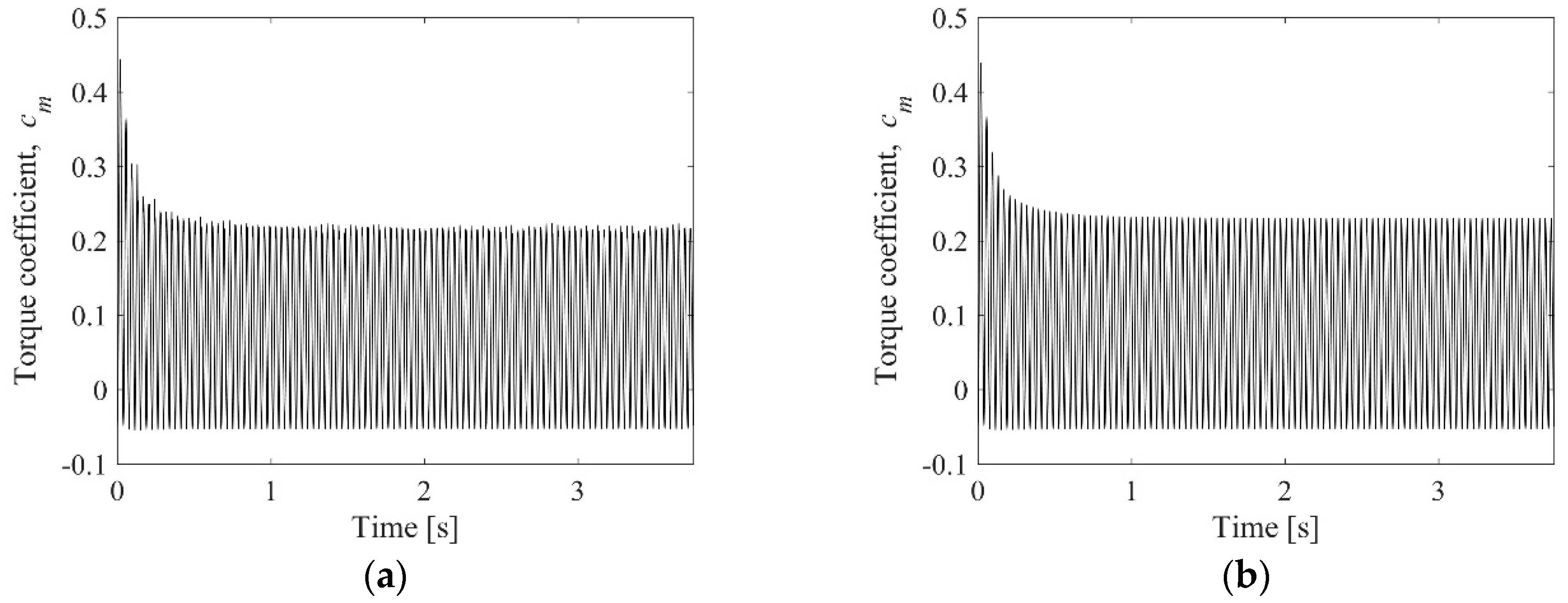
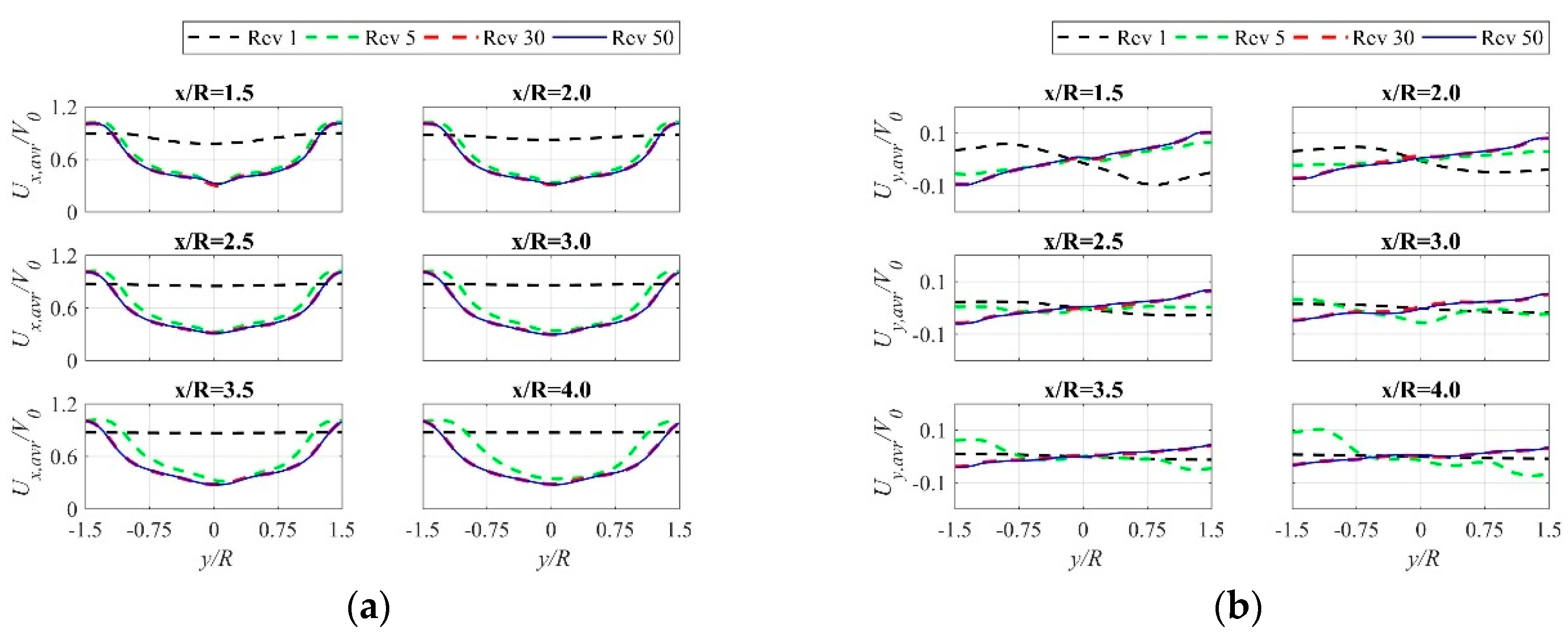
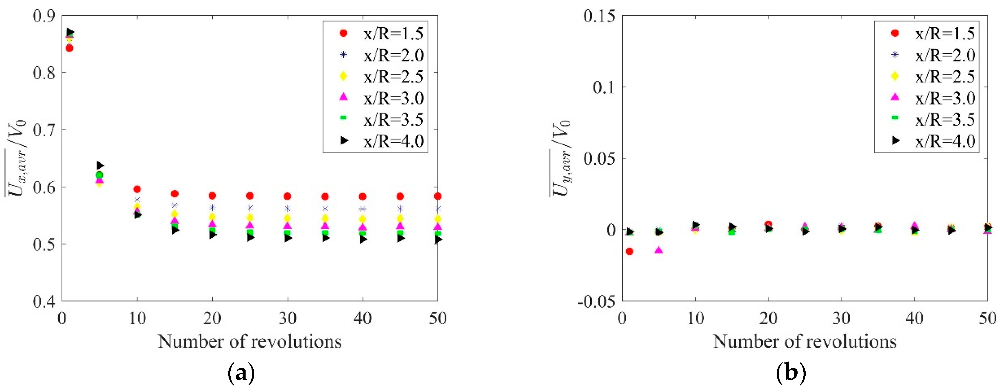
4.3. Revolution Convergence Analysis

Numerical calculations can be sensitive to certain factors. One of them is certainly homogeneous initial conditions in the whole computational domain that are assumed very often in numerical simulations. The calculation should continue until the transient flow characteristics and aerodynamic forces will be repeated in each successive rotation of the wind turbine rotor. In this work, 50 revolutions of the rotor were simulated for each case studied. Figure 11a–d show the aerodynamic forces calculated for several exemplary rotor revolutions. These results are given for the clean rotor and for the shafted rotor. In both cases, it can be noticed that after ten full revolutions the results are similar to those obtained for the 50 rotations of the rotor.

To answer the question of how many revolutions should be simulated to make the results repeatable, two graphs of torque coefficients as a function of time are presented (Figure 12). A time equal to 3.75 s corresponds to a time of 50 full rotor revolutions. These drawings show two very important things. First, the simulation of 10 full rotor revolutions is sufficient to obtain repeatable results of the torque coefficient. Secondly, unlike the clean rotor, torque coefficient results for a rotor equipped with a shaft are not identical for each subsequent rotation. The differences are very small, but they are visible even with the naked eye. These differences result from the frequency of aerodynamic forces on the rotor shaft, which is different from the frequency of aerodynamic forces acting on the rotor blades. The frequency of the aerodynamic force acting on the rotor blade is 13.33 Hz while in the case of the shaft it is equal to 28.48 Hz.

The product of the rotor torque coefficient, c_m, averaged over the entire rotation of the rotor and the tip speed ratio is called the rotor power coefficient C_P. This is an important physical quantity that allows to evaluate the aerodynamic efficiency of the wind turbine. Figure 13 shows the relation of the rotor power coefficient as a function of the number rotor revolutions simulated. It is worth noting that when the effect of initial conditions subsides, the power coefficient of the clean rotor is constant while in the case of a rotor with a shaft it is almost constant. The clean rotor achieves a power coefficient of 0.4109 while the shafted rotor of 0.401.

It is obvious that the number of rotor revolutions necessary to obtain repetitive results of aerodynamic forces is not sufficient to obtain reliable results of the velocity field downstream behind the rotor. It was decided in this work, to investigate the number of revolutions of the shafted rotor required to correctly calculate velocity profiles.

Figure 14a,b show the velocity profiles for six distances downstream behind the rotor and for four examples rotor rotations. It is clear from the presented drawings that the number of revolutions required for simulation depends on the distance from the rotor axis of rotation to the place where reliable results of the flow parameters are needed. In order to give the reader a clue about the number of necessary revolutions for his simulation, some additional analyses have been made. Velocity profiles for each x/R position were averaged in the y-axis direction, i.e., for y/R in the range of -1.5 to 1.5. The results obtained are shown in Figure 15a,b. Figure 15a clearly shows that the number of revolutions needed to obtain a reliable velocity profile is 10 for the position x/R = 1.5 and 20 for x/R = 4.0. This drawing is also valuable for one more reason. It shows that the velocity component parallel to the wind direction decreases along with the distance from the rotor axis of rotation, x/R. The average velocity along the profile x/R = 1.5 is 0.5832 and for x/R = 4.0 it is 0.5077. The rate of decreasing velocity is approximately linear. In the case of the second velocity component, its average values reach a value close to zero after 10 revolutions (Figure 15b).

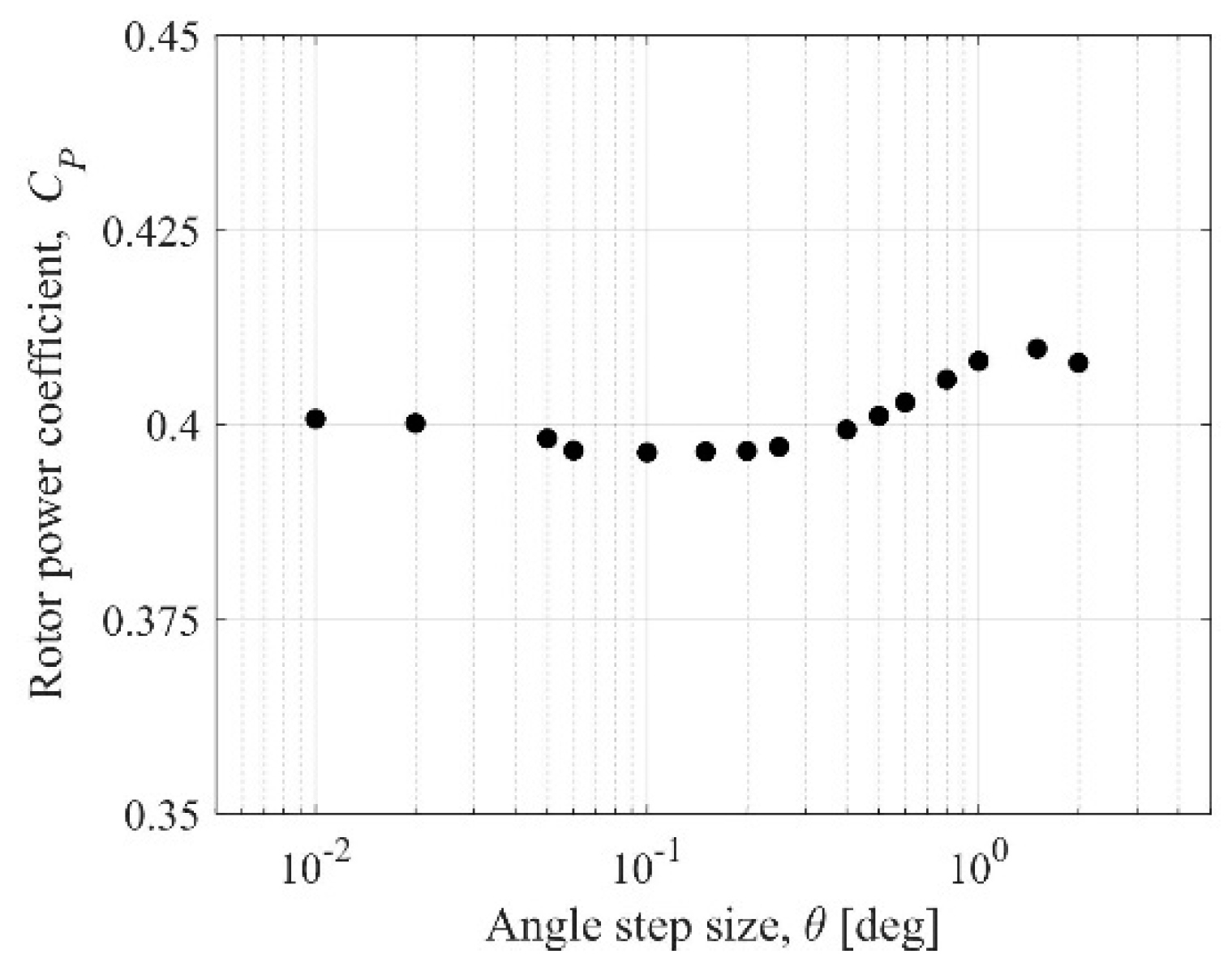
4.4. Impact of Time Step Size

In the case of transient numerical calculations, not only the influence of boundary conditions is important, but also the choice of the time step size. In the case of the solver employed, the time step size should be chosen in such a way that it satisfies the given convergence criteria. However, even if these criteria have been fulfilled, it may not be enough to analyze all phenomena. In the case of the analyzed problem, a number of time steps were taken into account. Since the specification of the time step in seconds is not intuitive, the time step corresponds to the increment of the rotation angle Δθ (deg) (angle step size). In this work, the angle step size is given in the range from 0.01 to 2.5 degrees. In each of the cases studied, repeatable results of flow parameters and aerodynamic blade loads were obtained. For the largest angle step size Δθ=2.5 deg the minimum convergence level of 10^-3 was obtained whereas for the smallest angle decrement Δθ=0.01 deg the minimum convergence level was 10^-5. During the research, it turned out that the selection of the appropriate time step size has the greatest impact on the estimation of the aerodynamic blade loads of the blade moving in the rotor shaft shadow, Figure 16a,b. The influence of the time step size on the rotor power coefficient is shown in Figure 17. Initially, as the time step size decreases, the power coefficient increases. This is related to a better estimation of the tangential blade loads in the upwind part of the rotor. Further reduction of the time step size leads to a reduction in the power coefficient which is related to the effect of the rotor shaft shadow. Below the time step size corresponding to the angle step size of 0.05 deg, the rotor power coefficient begins to be constant.

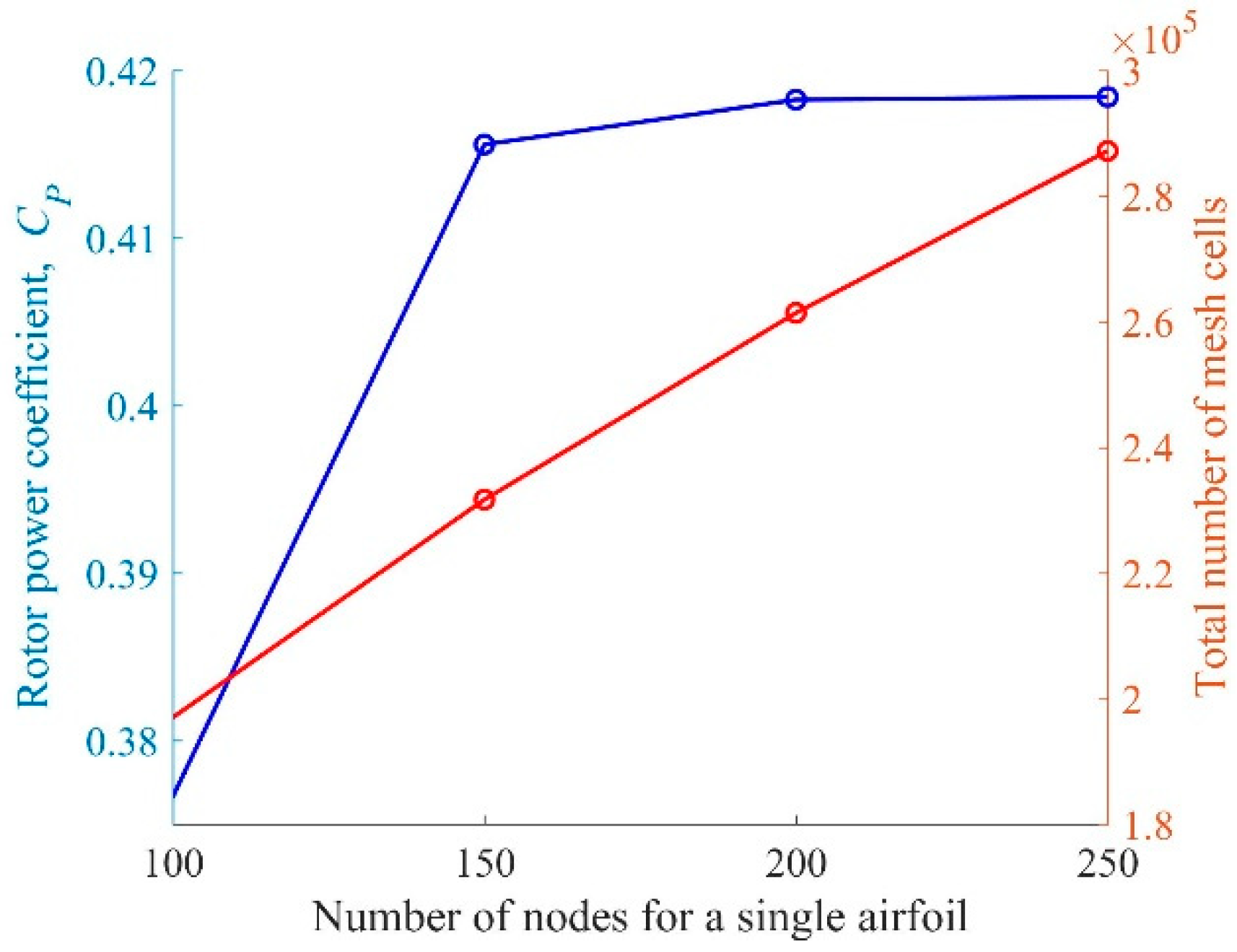
4.5. Mesh Convergence Study

The last factor that was analyzed in this work is the influence of the numerical grid density on the solution. Due to the time-consuming nature of the calculations, only one grid parameter was examined—the number of grid nodes on the profile edges. For the coarse grid, the number of identical divisions at the airfoil edges was 100, and in the case of a fine mesh, the number of divisions was 250. Figure 18 proves that in order to obtain the power coefficient independent of the number od division of the airfoil edges this number should be minimum 200. The increase in the number of divisions, however, is associated with the increase in computational effort because the linear increase in the number of divisions do the airfoil edges results in a nearly linear increase in the total number of grid elements from 196,992 to 287,186.

5. Conclusions

The purpose of this paper was to determine the aerodynamic blade loads of the Darrieus wind turbine using the URANS approach with the SST k-ω turbulence model. The velocity distributions in the rotor area and in the aerodynamic wake downstream behind the rotor were also investigated. On the basis of the results obtained, it was determined that:

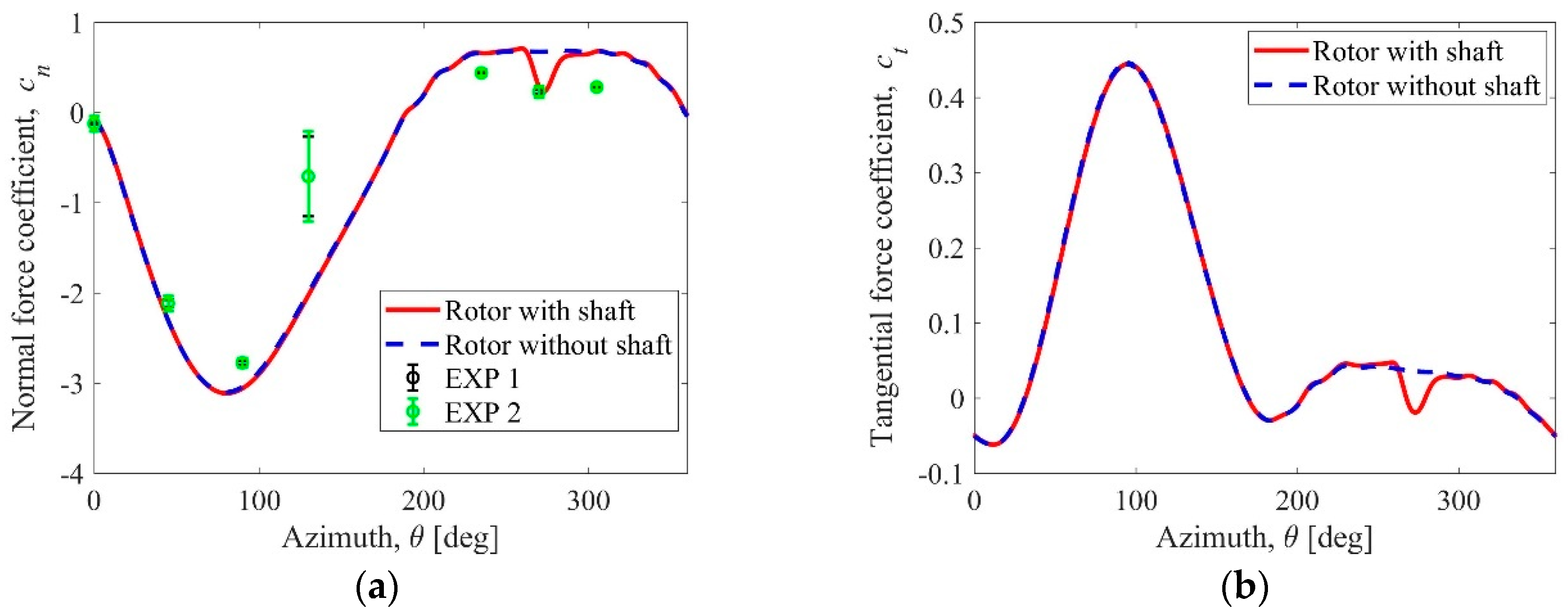
• The SST k-ω turbulence model provides the results of the normal aerodynamic force component that appears to be satisfactory by comparing it with experimental results. However, slightly overestimated results of this force component may be due to 3D effects, which are not included in this work.
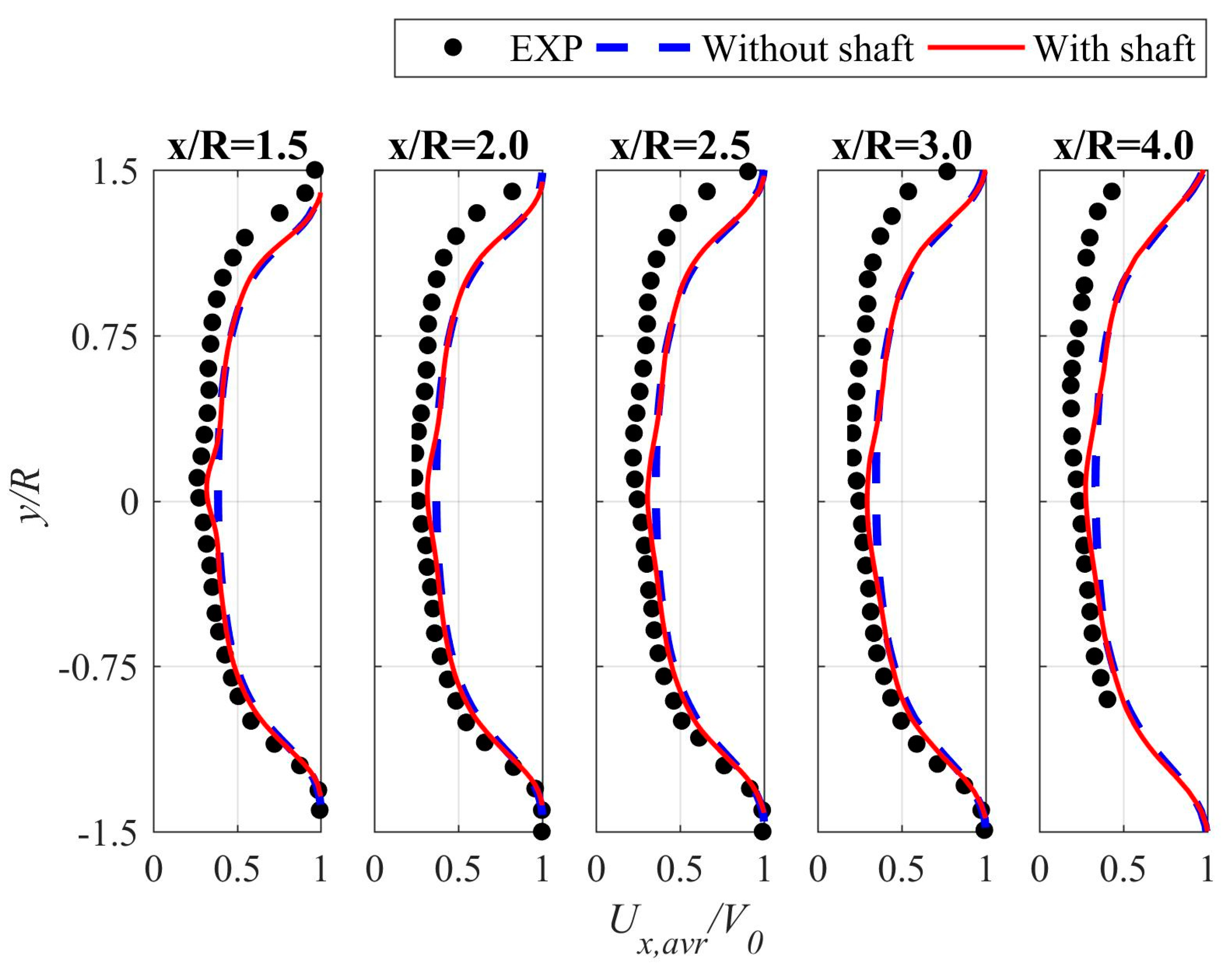
• The reason why the calculated velocity profiles (the velocity component parallel to the wind direction) downstream behind the rotor are not asymmetrical as in the case of the experimental studies it is not entirely clear. One possible reason is the simplification of the numerical model.
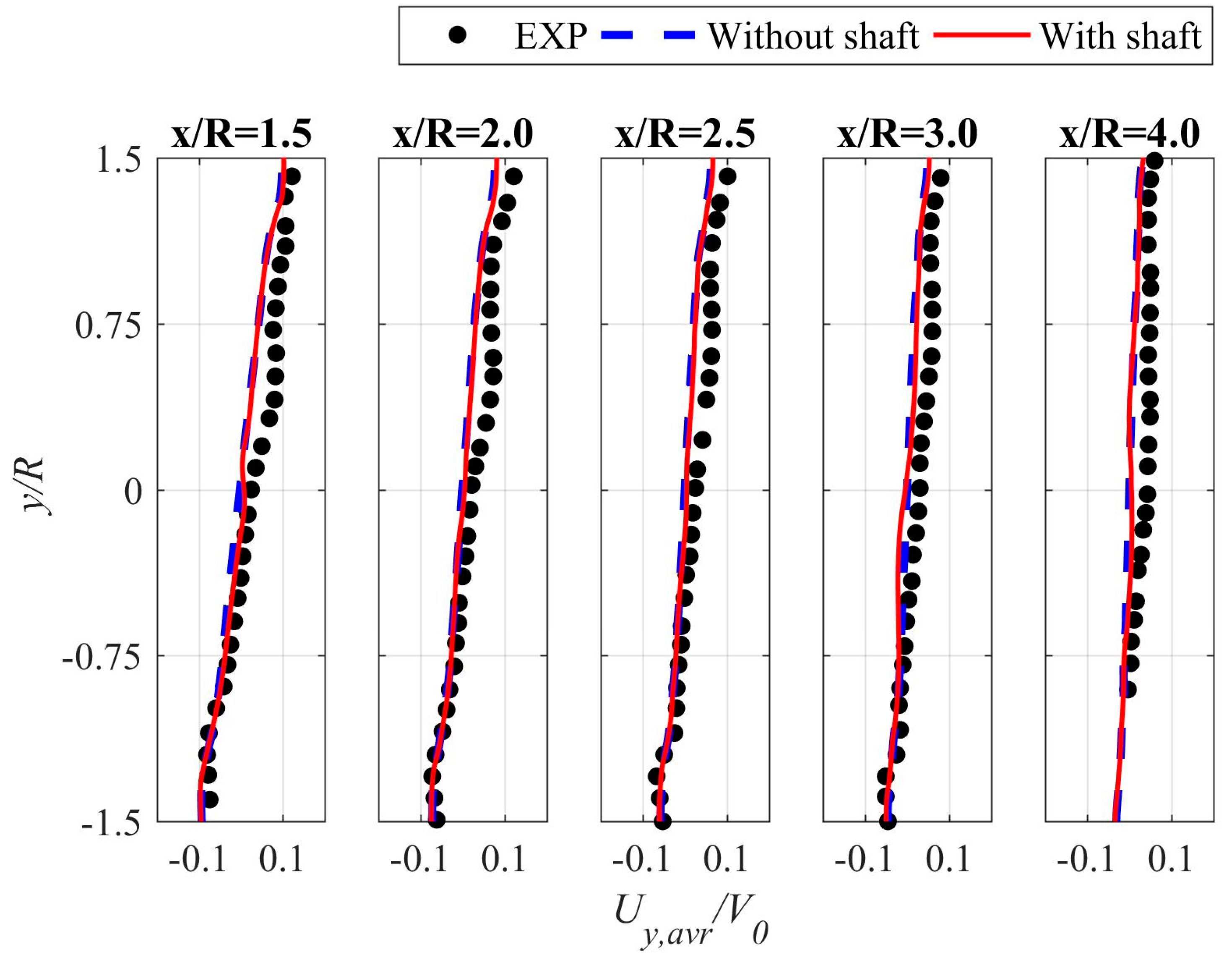
• The results of the second velocity component profiles agree much better with experimental research.
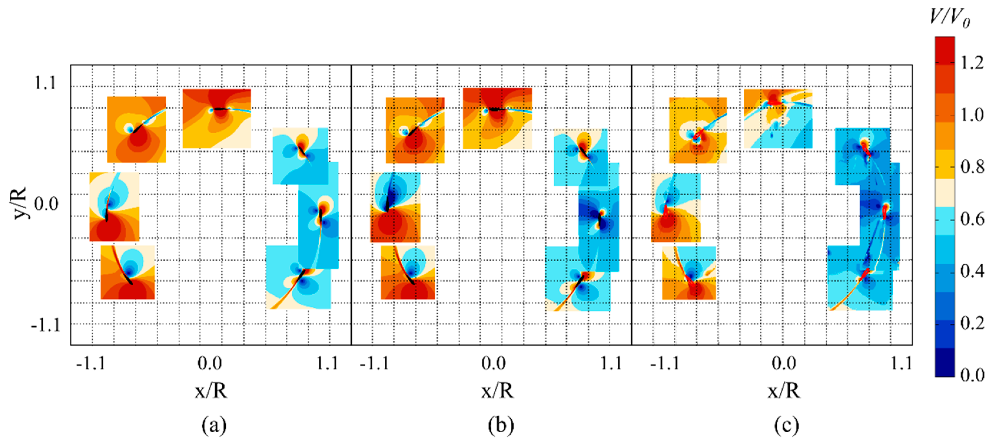
• The flow field around the wind turbine rotor is highly three-dimensional. The occurrence of flow separation is very likely in such conditions that are not favorable for URANS approach. Nevertheless, for the two-equation k-ω SST turbulence model and the URANS model, that were used here, the instantaneous velocity fields are consistent with the PIV studies.
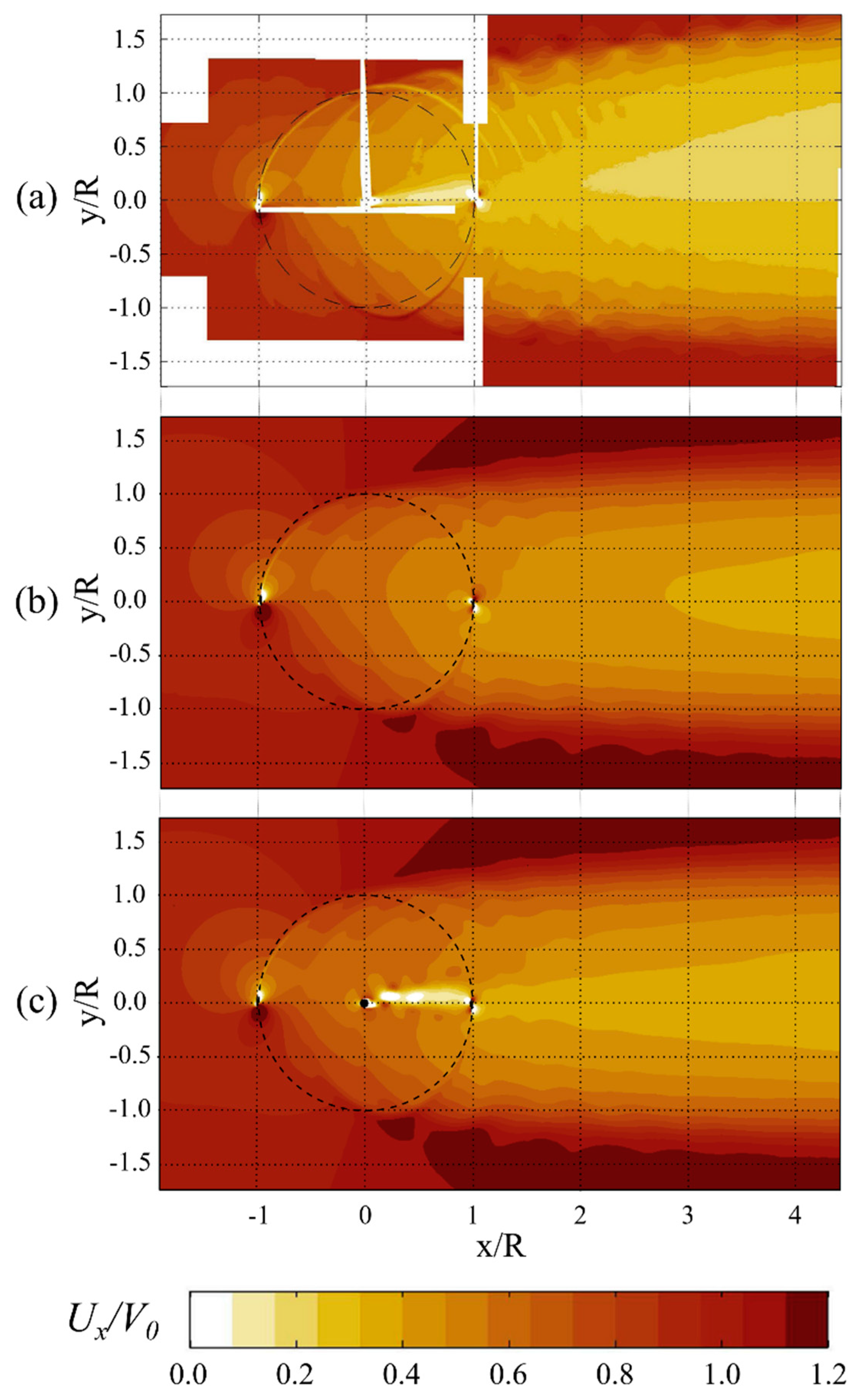
• The influence of the rotating shaft is visible mainly in the central part of the velocity profiles and rapidly decreases with the distance downstream from the axis of rotation.
• The drop in the mean velocity for each U_x velocity profile is linear for six distances x/R downstream behind the rotor from 1.5 to 4.0. The average value of the velocity component parallel to the wind direction decreased by 13% for the given x/R range.
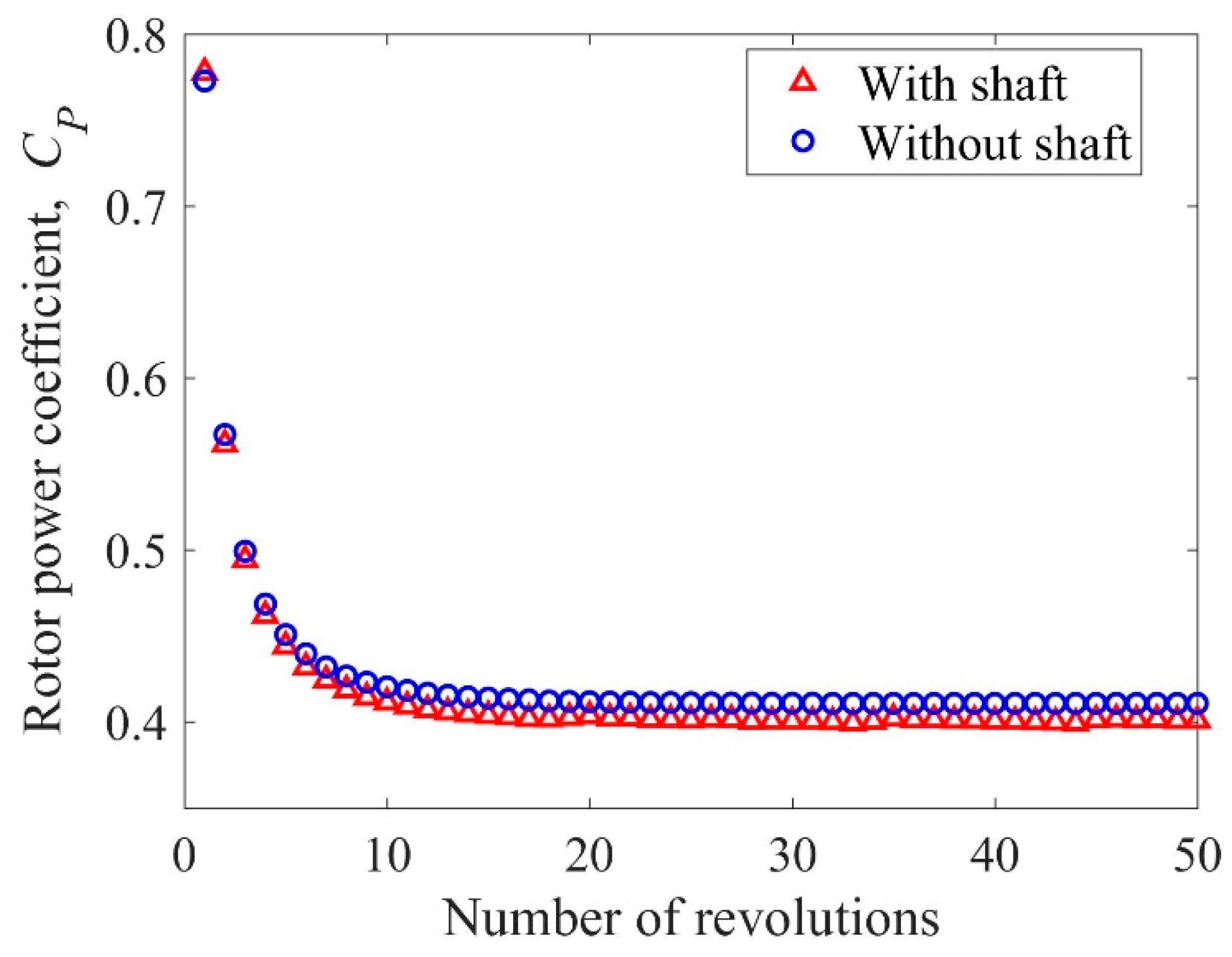
• The rotor in a non-shaft configuration achieves a power coefficient of 2.468% compared to a rotor equipped with a shaft.
• The frequency of the aerodynamic force acting on the shaft is 113.6% higher compared to the frequency of aerodynamic force of the rotor blade.
• Ten full rotor revolutions are sufficient to obtain repeatable results of the torque coefficient and almost constant values of the averaged rotor power coefficients. However, in order to obtain appropriate velocity profiles at the distance of 4R downstream behind the rotor, 15 full rotor revolutions are required for simulation.
• The selection of the appropriate time step size has the greatest impact on the estimation of the aerodynamic blade loads of the blade moving in the rotor shaft. If the time step size is too large, the shaft influence is invisible. Below the time step size corresponding to the angle step size of 0.05 degrees, the rotor power coefficient begins to be constant.

The research presented in this paper is a part of scientific project that aims to develop a new aerodynamic model for vertical-axis wind turbines with the Darrieus rotor. The results of instantaneous and average flow parameters presented in this article as well as the results of aerodynamic forces will be a benchmark for validation of the developed analytical method.

References

1. Santoni, C.; Carrasquillo, K.; Arenas-Navarro, I.; Leonardi, S. Effect of tower and nacelle on the flow past a wind turbine. Wind Energy 2017, 20, 1927–1939. [Google Scholar] [CrossRef]
2. Hansen, M.O.L.; Madsen, H.A. Review paper on wind turbine aerodynamics. J. Fluids Eng. 2011, 133, 114001. [Google Scholar] [CrossRef]
3. Cai, X.; Gu, R.; Pan, P.; Zhu, J. Unsteady aerodynamic simulation of a full-scale horizontal axis wind turbine using CFD methodology. Energy Convers. Manag. 2016, 112, 146–156. [Google Scholar] [CrossRef]
4. Paraschivoiu, I. Wind Turbine Design—With Emphasis on Darrieus Concept; Polytechnic International Press: Montreal, QC, Canada, 2002. [Google Scholar]
5. Paraschivoiu, I.; Delclaux, F. Double multiple streamtube model with recent improvements. J. Energy. 1983, 7, 250–255. [Google Scholar] [CrossRef]
6. Paraschivoiu, I.; Delclaux, F.; Fraunie, P.; Beguier, C. Aerodynamic Analysis of the Darrieus Rotor Including Secondary Effects. J. Energy 1983, 7, 416–422. [Google Scholar] [CrossRef]
7. Beri, H.; Yao, Y. Double multiple streamtube model and numerical analysis of vertical axis wind turbine. Energy Power Eng. 2011, 3, 262–270. [Google Scholar] [CrossRef]
8. Lazauskas, L. Three pitch control systems for vertical axis wind turbines compared. Wind Eng. 1992, 16, 269–282. [Google Scholar]
9. Klimas, P.C. Proceedings of the Vertical Axis Wind Turbine (VAWT) Design Technology Seminar for Industry; Technical Report SAND80-0984; Sandia National Laboratories: Albuquerque, NM, USA, 1948.
10. Wang, Z.; Wang, Y.; Zhuang, M. Improvement of the aerodynamic performance of vertical axis wind turbines with leading-edge serrations and helical blades using CFD and Taguchi method. Energy Convers. Manag. 2018, 177, 107–121. [Google Scholar] [CrossRef]
11. Lam, H.; Peng, H. Study of wake characteristics of a vertical axis wind turbine by two- and three-dimensional computational fluid dynamics simulations. Renew. Energy 2016, 90, 386–398. [Google Scholar] [CrossRef]
12. Li, C.; Zhu, S.; Xu, Y.L.; Xiao, Y. 2.5 D large eddy simulation of vertical axis wind turbine inconsideration of high angle of attack flow. Renew. Energy 2013, 51, 317. [Google Scholar] [CrossRef]
13. Castelli, M.R.; Benini, E. Effect of blade inclination angle on a Darrieus wind turbine. J. Turbomach. 2012, 134, 031016. [Google Scholar] [CrossRef]
14. Lanzafame, R.; Mauro, S.; Messina, M. 2D CFD modeling of H-darrieus wind turbines using a transition Turbulence Model. Energy Procedia 2014, 45, 131–140. [Google Scholar] [CrossRef]
15. Shamsoddin, S.; Porté-Agel, F. Large eddy simulation of vertical axis wind turbine wakes. Energies 2014, 7, 890–912. [Google Scholar] [CrossRef]
16. Rezaeiha, A.; Montazeri, H.; Blocken, B. Towards accurate CFD simulations of vertical axis wind turbines at different tip speed ratios and solidities: Guidelines for azimuthal increment, domain size and convergence. Energy Convers. Manag. 2018, 156, 301–316. [Google Scholar] [CrossRef]
17. Bangga, G.; Lutz, T.; Jost, E.; Krämer, E. CFD studies on rotational augmentation at the inboard sections of a 10MW wind turbine rotor. J. Renew. Sustain. Energy 2017, 9, 023304. [Google Scholar] [CrossRef]
18. Bangga, G.; Hutomo, G.; Wiranegara, R.; Sasongko, H. Numerical study on a single bladed vertical axis wind turbine under dynamic stall. J. Mech. Sci. Technol. 2017, 31, 261–267. [Google Scholar] [CrossRef]
19. Alaimo, A.; Esposito, A.; Messineo, A.; Orlando, D.; Tumino, D. 3D CFD Analysis of a Vertical Axis Wind Turbine. Energies 2015, 8, 3013–3033. [Google Scholar] [CrossRef] [Green Version]
20. Rogowski, K. Numerical studies on two turbulence models and a laminar model for aerodynamics of a vertical-axis wind turbine. J. Mech. Sci. Technol. 2018, 32, 2079–2088. [Google Scholar] [CrossRef]
21. Rogowski, K.; Hansen, M.O.L.; Lichota, P. 2-D CFD Computations of the Two-Bladed Darrieus-Type Wind Turbine. J. Appl. Fluid. Mech. 2018, 11, 835–845. [Google Scholar] [CrossRef]
22. Wekesa, D.W.; Wang, C.; Wei, Y.; Kamau, J.N.; Danao, L.A. A numerical analysis of unsteady inflow wind for site specific vertical axis wind turbine: A case study for Marsabit and Garissa in Kenya. Renew. Energy 2015, 76, 648–661. [Google Scholar] [CrossRef]
23. Rezaeiha, A.; Montazeri, H.; Blocken, B. On the accuracy of turbulence models for CFD simulations of verticalaxis wind turbines. Energy 2019, 180, 838–857. [Google Scholar] [CrossRef]
24. Rezaeiha, A.; Kalkman, I.; Montazeri, H.; Blocken, B. Effect of the shaft on the aerodynamic performance of urban vertical axis wind turbines. Energy Convers. Manag. 2017, 149, 616–630. [Google Scholar] [CrossRef]
25. Zhang, L.; Zhu, K.; Zhong, J.; Zhang, L.; Jiang, T.; Li, S.; Zhang, Z. Numerical Investigations of the Effects of the Rotating Shaft and Optimization of Urban Vertical Axis Wind Turbines. Energies 2018, 11, 1870. [Google Scholar] [CrossRef]
26. Tescione, G.; Ragni, D.; He, C.; Simão Ferreira, C.J.; van Bussel, G.J.W. Near wake flow analysis of a vertical axis wind turbine by stereoscopic particle image velocimetery. Renew. Energy 2014, 70, 47–61. [Google Scholar] [CrossRef]
27. Castelein, D.; Ragni, D.; Tescione, G.; Simão Ferreira, C.J.; Gaunaa, M. Proceedings of the 33rd Wind Energy Symposium; AIAA 2015-0723; American Institute of Aeronautics and Astronautics: Reston, VA, USA, 1963. [Google Scholar]
28. Menter, F.R. Two-Equation Eddy-Viscosity Turbulence Models for Engineering Applications. AIAA J. 1994, 32, 1598–1605. [Google Scholar] [CrossRef]
29. Barth, T.; Jespersen, D. The design and application of upwind schemes on unstructured meshes. In Proceedings of the 27th Aerospace Sciences Meeting, Reno, NV, USA, 9–12 January 1989; Paper 89-0366. AIAA: Reston, VA, USA, 1963. [Google Scholar] [CrossRef]
30. FLUENT Manual—ANSYS Release Version 17.1, Theory Guide; ANSYS, Inc.: Cannonsburg, PA, USA, 1970.
31. Strickland, J.H.; Webster, B.T.; Nguyen, N. A Vortex Model of the Darrieus Turbine: An Analytical and Experimental Study. J. Fluids Eng. 1979, 101, 500–505. [Google Scholar] [CrossRef]
32. Laneville, A.; Vittecoq, P. Dynamic Stall: The Case of the Vertical Axis Wind Turbine. J. Sol. Energy Eng. 1986, 108, 141–145. [Google Scholar] [CrossRef]
33. Rogowski, K.; Hansen, M.O.L.; Maroński, R.; Lichota, P. Scale Adaptive Simulation Model for the Darrieus Wind Turbine. J. Phys. Conf. Ser. 2016, 753, 022050. [Google Scholar] [CrossRef]
Figure 1. H-Darrieus wind turbine rotor and analyzed quantities. (a) Silhouette of the H-type Darrieus wind turbine; (b) Aerodynamic forces acting on the wind turbine blade and velocity components in the aerodynamic wake downstream behind the rotor.
Energies 12 02506 g001
Figure 2. Aerodynamic model of the two-dimensional H-Darrieus wind turbine.
Energies 12 02506 g002
Figure 3. Boundary conditions as well as computational domain and basic dimensions.
Energies 12 02506 g003
Figure 4. Grid distribution. (a) Mesh density in the rotor area; (b) Mesh around the blade; (c) Grid near the rotating shaft.
Energies 12 02506 g004
Figure 5. Aerodynamic blade loads. (a) Normal force component; (b) tangential force component.
Energies 12 02506 g005
Figure 6. Velocity profiles of the Ux component at a few x/R locations downstream behind the rotor.
Energies 12 02506 g006
Figure 7. Velocity profiles of the Uy component at a few x/R locations downstream behind the rotor.
Energies 12 02506 g007
Figure 8. Contour maps of the magnitude velocity around one blade for seven azimuthal positions given for (a) the rotor without shaft; (b) the rotor with shaft; (c) PIV [27].
Energies 12 02506 g008
Figure 9. Contour maps of the Ux velocity component, shown for (a) PIV [26]; (b) the rotor without shaft; (c) the rotor with shaft.
Energies 12 02506 g009
Figure 10. Contour maps of the Uy velocity component, shown for (a) PIV [26]; (b) the rotor without shaft; (c) the rotor with shaft.
Energies 12 02506 g010
Figure 11. Aerodynamic forces for example rotor rotations. (a) Normal force coefficient for clean rotor; (b) Tangential force coefficient for clean rotor; (c) Normal force coefficient for the shafted rotor; (d) Tangential force coefficient for the shafted rotor.
Energies 12 02506 g011
Figure 12. Torque coefficient from the entire rotor for: (a) the rotor with shaft; (b) the clean rotor.
Energies 12 02506 g012
Figure 13. History of the rotor power coefficient for the shafted rotor and the clean one.
Energies 12 02506 g013
Figure 14. Velocity profiles for example rotor rotations: (a) Ux velocity component; (b) Uy velocity component.
Energies 12 02506 g014
Figure 15. Averaged velocity profiles for different positions downstream behind the rotor for (a) Ux velocity component; (b) Uy velocity component.
Energies 12 02506 g015
Figure 16. Influence of the time step size that corresponds to the angle step size Δθ on the aerodynamic blade loads: (a) normal and (b) tangential.
Energies 12 02506 g016
Figure 17. Influence of the time step size (the angle step size Δθ) on the rotor power coefficient.
Energies 12 02506 g017
Figure 18. Influence of mesh density on the rotor power coefficient and the total number of grid elements.
Energies 12 02506 g018