Abstract
The wind energy conversion system (WEC) has been increasingly proposed to capture wind energy producing electrical power in high efficiency. One of the most important factors that has significant influence on the overall efficiency is the performance of generators in a fixed-speed wind turbine. The efficiency of the generator strongly depends on the operating speed. Therefore, the generator should be controlled to operate at the rated speed to increase the overall efficiency. In this paper, a continuously variable transmission (CVT) was employed to maintain the speed of the generator by controlling the transmission ratio. By employing a position control system based on an electro-hydraulic actuator (EHA), the speed ratio could be tuned continuously to keep the generator at rated speed. Here, an adaptive fuzzy sliding mode control (AFSC) was developed to control the proposed EHA CVT. Mathematical analysis was also carried out to investigate the global stability of the system. Finally, experiments were conducted to evaluate the performance of the proposed WECs.
1. Introduction
Finding sustainable energy becomes more and more urgent nowadays due to the rapid exhaustion of fossil fuel resources and the unfailingly intensifying of energy demand. Alternative energy resources include solar, wind, tidal, wave, biomass energies, etc. Among these resources, the number of wind energy conversion technologies has speedily increased as well as the number of researches to maximize the power and efficiency of wind energy conversion systems (WECs) [1,2,3].
The idea of converting wind energy into useful energy has continuously developed for a thousand years. A wind turbine extracts kinetic energy from the wind and converts it into mechanical energy. This mechanical energy then drives the generator to produce electrical power. There are several methods to optimize the efficiency of a wind turbine. Among them, some researchers propose the variable speed generator to produce the electric power, then the frequency converter or other techniques are applied to adjust the current frequency into the fixed frequency of the grid [4,5]. However, developing a high efficiency generator for a variable speed input is a very complex task and it increases the cost. Hence, the more effective methodology to maximize the amount of extracted wind energy is to keep the generator at an optimal speed. This has been an appealing research trend around the world [6,7,8,9]. The wind speed always varies, but the conventional wind system can only produce the power within “cut in” and “cut out” of the wind speed [10]. There are several methods that can be control the speed, such as pitch control, stall control, yaw control, and combinations of the above methods [11,12]. However, these methods need a complex mechanism to control the pitch angle and yaw angle.
National Renewable Energy Laboratory’s previous studies have shown the advantages of a continuously variable transmission (CVT) in the wind turbine, as reliable and efficient [7,8], reducing the cost of energy production up to 11.2% [13]. The automatically regulated CVT and CVT with a hydraulic system used in the above studies have faced disadvantages of mass practical adoption in WECs. For example, the automatically regulated CVT only works under the low torque condition, while in WECs the CVT also needs to cope with the high torque range. Meanwhile, conventional hydraulic system wastes a lot of energy through the control valves thus it decreases the overall efficiency of the hydraulic CVT system. Consequently, development of the new CVT system to improve the performance of the wind turbine is necessary.
In this paper, an electro-hydraulic actuator (EHA) CVT is proposed. When the speed of the generator is at the rated value, the hydraulic circuit inside the EHA locks the current axial position of the CVT and thus keeps the CVT ratio constant without consuming energy. Then, a control strategy for the CVT was developed, and a mathematical model of the wind turbine system was derived. Based on the input speed of the CVT and the input speed conditions of the generator, the position-reference command for an EHA was generated. Due to the nonlinearities and uncertainties of the CVT as well as the EHA, a fixed gains proportional-integral-derivative (PID) controller [14] cannot yield reasonable performance over a wide range of operating conditions [15]. Therefore, many advanced control approaches such as fuzzy PID [16,17], sliding mode [18,19], adaptive back-stepping [20] and iterative back-stepping [21] have been developed for similar systems.
Among the above control strategies, a well-known methodology is the sliding mode control technique. However, the common drawback of the conventional sliding mode control, which is the chattering phenomenon due to the use of discontinuous sign function [18,19], was overcome by employing a fuzzy logic turning mechanism in many studies [22,23,24]. The fuzzy sliding mode control also has more robustness against parameters’ variation [15,22]. To simplify the designing phase of the fuzzy logic mechanism, an adaptive fuzzy controller based on the Lyapunov synthesis approach was studied in [23,24]. In such controllers, the fuzzy rules can be automatically adjusted to achieve a satisfactory response due to adaptive laws [25]. To improve the control performance, a PID-like fuzzy sliding mode control approach was recently introduced [26,27,28]. This control strategy inherits the properties of both PID and sliding mode approaches and thus provides better tracking performance. Thus, it is employed in control of hydrostatic transmission system [26], hydraulic servo systems [27] and a simulated uncertain system [28]. In this paper, a similar methodology is used to develop the controller for the proposed EHA CVT in WECs. The control signal includes a PID-like sliding mode control signal ɷeq and a fuzzy hitting control signal ɷhit to allow both a fast reaching and smooth tracking response. All the control parameters were updated carefully, satisfying Lyapunov criteria, to ensure global stability.
Finally, experimental tests were also carried out to evaluate the performance of the proposed WECs. The wind speed was captured from experimental data at an average value of 10 m/s with the variation amplitude up to ±4 m/s. Experimental tests showed that the proposed system was able to drive the generator at a stable speed of 250 rpm and thus generate a constant power of 10.5 kW at the generator efficiency of 92%. These results strongly confirmed the potential of the proposed WECs for practical application.
2. Description of System
Figure 1 illustrates the schematic of a new wind turbine design which typically consists of a rotor, gearbox, EHA CVT and a generator. The horizontal wind turbine is composed of three huge blades to convert wind flow into rotary motion of the shaft. The main limitation of this wind turbine rotor is its low and variable operating speed which is inappropriate with the high speed (200–3600 rpm) of the generator. Thus, a gear box was attached to amplify low speed of the wind turbine rotor to the operational speed range of the generator [6]. Then, the output shaft of the gearbox was connected to the driving axis of the EHA CVT.
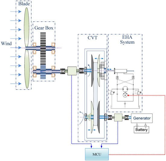
Figure 1.
Configuration of experiment test rig.
The main purpose of a CVT is to transform the variable speed of the primary unit into a stable rotary speed at the secondary unit (Figure 2). The primary unit includes a primary shaft, a primary driving moveable conical disk moving axially on the primary shaft, and a driving hydraulic cylinder. The driving moveable conical disk is axially moved by a supplied oil pressure chamber and resistive force of belt [29]. Since the belt is sandwiched between the driving moveable conical disk and driving fixed conical disk, it transmits rotary speed into the secondary unit. Similarly, the secondary unit includes a secondary-driven moveable conical disk supplied force by the spring and a driven fixed conical disk. The secondary shaft then directly drives the generator. In this paper, the position of the primary axis of the CVT is controlled by a pump controlled EHA. Particularly, the EHA is employed to control the oil pressure inside the chambers by supplying or disposing flow by the hydraulic pump to control the primary pulley position of the CVT. The EHA system includes a gear pump, a supplementary valves system, and a symmetrical acting cylinder. The whole system is driven by a DC motor. In this configuration, the movement of the cylinder is adjusted directly by the speed of the DC motor [21]. By controlling the position of the primary pulley, transmission ratio of the CVT as well as the input speed of the generator can be controlled.
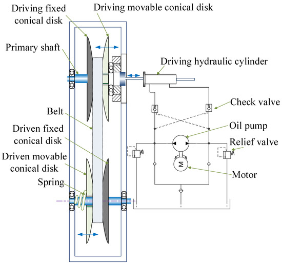
Figure 2.
Electro-hydraulic actuator (EHA) continuously variable transmission (CVT) system.
3. System Modeling and Problem Statement
3.1. Wind Model
Generally, there are four operation regions for the wind turbine as shown in Figure 3. In region 1, wind speed is not large enough to turn the wind turbine blade, thus the rotor is standing still. If wind speed is large enough to overcome the friction in the turbine as well as the loading torque of the generator to start turning turbine blade, the system enters region 2. In this region, the turbine blade should be maintained at an optimal speed to maximize the energy converter. In region 3, the power production of the turbine is limited because the generator is already at maximum power. In region 4, the turbine is stopped to avoid damage at high wind speeds.
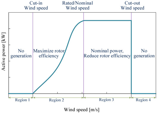
Figure 3.
Turbine power curve.
The model of the wind turbine can be described as follows. Firstly, the power (PWT) captured by the wind turbine blades is expressed:
where is air density (typical 1.225 kg/m3), A is the swept area of the blade in m2, is the wind velocity in m/s and Cp is power capture coefficient which is a function of tip speed ratio and pitch angle . The power coefficient Cp is calculated as in [30]:
with
where the coefficients C1 to C6 are: C1 = 0.5176, C2 = 116, C3 = 0.4, C4 = 5, C5 = 21 and C6 = 0.0068. The tip speed ratio of the wind turbine λ is defined as following [10]:
here, R is the rotor radius in m, is the angular velocity of the rotor in rad/s.
Figure 4 presents the power coefficient versus the tip speed ratio and pitch angle. It can be seen that with the pitch angle the blade is 0° and the maximum coefficient of power (Cp = 0.48) is achieved at the tip speed ratio = 8.1. This ratio value is considered as the optimal value. Hence, for each wind speed within the operation region 2, there exists an optimal rotor speed to maximize the output power of the wind turbine. The optimal speed of the rotor is calculated as follows:
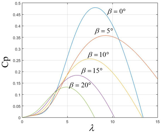
Figure 4.
Power coefficient with respect to tip speed ratio and pitch angle.
When the air flows over the blade, it creates two types of aerodynamic force: one in the direction of the airflow (known as drag force) and the other perpendicular to the air flow (known as lift force). These forces can be used to generate the driving torque needed to rotate the blades [4]. In proportion to these forces, the wind speed fluctuations can be calculated by a statistic function with a power spectrum represented [31]:
where, are the lateral and longitudinal components of the wind speed, is the spectral power density, is the frequency spacing, is the random phase angle, is the number of frequencies.
with as the height above the ground, is the coefficient. The total vector of the horizontal wind is given by:
3.2. CVT Modeling
The CVT consists of a primary pulley, a secondary pulley and a belt connecting these two pulleys. The CVT geometry schematic diagram is given in Figure 5. By assuming that the belt elongation has not occurred during operation [29], the belt lengths can be calculated as in [32,33]:
where are the primary and secondary pulley running radii; are the angle of lap on the primary and secondary pulley; D is the pulley center distance.
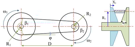
Figure 5.
Geometrical description of a belt CVT drive.
Other relations can be calculated as:
where is half of the increase in the wrapped angle on the primary pulley.
Substitute Equations (9) and (10) into Equation (8), one can obtain:
The relationship between the running radii and CVT ratio can be given as follows [29]:
A combination of Equations (11) and (12) allows us to obtain the following relation between and
In order to break an implicit loop, we use in the code the derivative of this expression:
From Equations (13) and (14) the sheave pulley displacement of the primary is calculated as:
The axial pulley positions are presented as follows [29]:
where are the minimum secondary and primary running radii.
are the secondary and primary pulley position.
is the pulley wedge angle.
The relationship between speed and running radii [29] is:
From Equations (12), (16), and (18), the ratio of the speed can be given as follows:
3.3. EHA Modeling
The modeling of an EHA was introduced in our previous study [21]. By using Newton’s second law and principles of hydraulic systems [15], the dynamics of load shaft in loading an EHA can be described by the following state space [29]:
where are the position, velocity, and acceleration of the hydraulic piston, respectively, is the loading accelerator term, is the equivalent mass, is the effective bulk modulus of the hydraulic fluid, are the initial volume of the two chambers, is the actuating area, Dp is the displacement of the pump, and ω is the input speed of the pump system, and are the parameters of leakage and supplementary valves, respectively. For more information, please refer to [20,21].
For simplification, the last equation of the state space can be rewritten as .
Obviously, system states are adjusted by the speed of the bi-directional pump that is driven by a DC servo motor. Consequently, the control signal is the speed command for the DC servo motor to control the output speed of the generator [21]. The development of a position controller will be described in the following section [15].
4. Control Design
The output speed is selected according to the power take-off system’s specification and wind conditions at a steady state. Based on the speed of the primary shaft and speed references of the secondary shaft of the CVT, the position command is computed for the EHA. The control signal for the EHA in this paper was calculated based on an adaptive fuzzy sliding mode control scheme. Firstly, an adaptive sliding mode is designed for the strictly feedback state space of the EHA system. Then, the fuzzy learning approach is employed to form the virtual control signal. The procedure of designing the controller is presented as follows [15].
The design of a sliding controller involves two steps. The first step is to design a stable sliding surface to achieve the control objective. The second step is to make the sliding surface attractive by pushing the system states toward the surface [15].
Let the system tracking error be defined as [15]:
where is the desired position of the EHA, is the response of the system which can track the desired position. Then a sliding surface is defined as:
The derivative of Equation (22) is:
Then we have
From Equations (23) and (24), we have
Coefficient is strictly positive. The term in Equation (25) is unknown but bounded
where is the bounded value and is the compensative value of .
Equation (25) can be shown as:
where is a lumped function and unknown.
In a proper control system, . Assuming that the system parameters are well-known, and the external disturbance is measurable (), the optimal equivalent controller for the position control of the system can be derived as:
The equivalent control effort of angular velocity of the DC motor can be calculated as:
Due to f(t) unknown, Equation (29) cannot be used to calculate the equivalent control effort. Therefore, this control effort is approximated as following:
is control gain to be designed. In this paper, the equivalent control, Equation (30), can be calculated by an adaptive approximator as follows:
where is an adaptive gain; and is a regressive term.
We assume that the equivalent control of Equation (30) can be expressed via Equation (31) as follows:
where is the ideal value of the adaptive gain; is the inherent approximation error.
The auxiliary control effort is designed as
From Equations (31) and (33), the angle velocity is
From Equation (25) we have
From Equations (19) and (22) we have
Consider a Lyapunov function as
where is a desired bound of the surface in infinite time, is a scaled gain, are positive constants.
Then we have
It is obvious that if the error is approximately equal to zero, and will be smaller than zero. Thus
Then we have
In order to satisfy the stability condition outside the domain , the positive constant η must be satisfied in the following condition
Equation (41) reveals that the value of depends on the upper bound of the function .
As shown in Equation (25), the bound of Δg is estimated but in practical application it is difficult to obtain accurately. Further, ε is an unknown value. Therefore, the bound of is also difficult to obtain precisely. If the bound chosen is too small, the stability condition cannot be satisfied; in contrast if the bound of chosen is too large, the hitting control action will cause serious chattering phenomenon and this phenomenon will excite an unstable system dynamic. Hence, we consider that the bound of the function is unknown.
To reduce the influence of the chattering phenomenon, a saturation function is used as
where is the thickness of the boundary layer.
However, likewise to the above problem, the positive constant in Equation (42) also depends on the bound of . So, the stability inside the boundary layer cannot be guaranteed.
To solve this, in this research, a fuzzy logic algorithm is employed to determine the hitting control action (ɷhit). Here, the sliding surface s is the input linguistic variable of the fuzzy logic and the hitting control action is the output linguistic variable. Seven linguistic states of the linguistic input and output variable are negative big (N03), negative medium (N02), negative small (N01), zero (ZE), positive small (P01), positive medium (P02), and positive big (P03). The membership function for the linguistic input and output variable is shown in Figure 6.
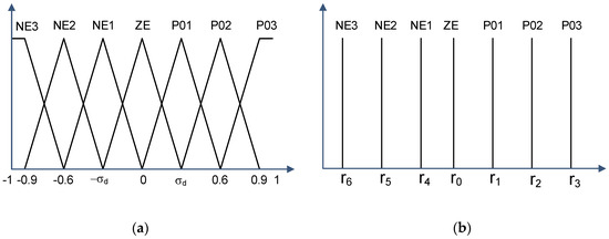
Figure 6.
The membership functions for: (a) the input variable s and (b) the output variable ωhit.
According to the hitting control action given by Equation (42), the basic rules of the fuzzy system are constructed as follows:
- Rule 1: If s is the ZE then ɷhit is the ZE
- Rule 2: If s is the P01 then ɷhit is the P01
- Rule 3: If s is the P02 then ɷhit is the P02
- Rule 4: If s is the P03 then ɷhit is the P03
- Rule 5: If s is the N01 then ɷhit is the N01
- Rule 6: If s is the N02 then ɷhit is the N02
- Rule 7: If s is the N03 then ɷhit is the N03
Then, the resulting discrete of the output variable can be obtained by using the center-average method as
where, 0 ≤ μi ≤ 1, i = 0, 1, …, 6 are the firing strengths of rules 1, 2, …, 7. r0, r1, r2, r3, r4, r5, r6 are the center of the membership function ZE, P01, P02, P03, N01, N02, N03 of the output variable, respectively. Here we choose as follows
where r is the fuzzy parameter. Due to , Equation (42) can be rewritten as
with .
r0 = 0, r1 = r, r2 = 2r, r3 = 3r, r4 = −r, r5 = −2r, r6 = −3r
As shown, when s > 0 then , oppositely when s < 0 then . Therefore, .
It is also noted that .
By replacing ωhit in Equation (34) by Equation (44), the time derivative of the sliding surface is rewritten as
In order to satisfy the sliding condition, the fuzzy parameter r must satisfy the following condition [34].
According to Equation (46), there exists an optimal value r* to satisfy the sliding condition [34]
where is the positive constant.
However, the optimal value of r* is very difficult to determine accurately, so we use a simple adaptive algorithm to estimate the optimal value of r*. The final control law of the adaptive fuzzy sliding mode control (AFSC) is presented as
here, is the estimative value of the optimal value r*.
Finally, the AFSC was designed as shown in Figure 7. By using Equation (48), the proposed controller can satisfy the condition or the closed loop system is stable.
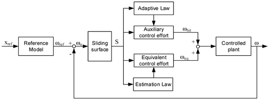
Figure 7.
Proposed adaptive fuzzy sliding mode control (AFSC) for position of EHA CVT system.
5. Experimental Evaluation
5.1. Experimental Test Rig
A test rig was set up to carry out the experimental works. The purpose of this experiment was to investigate the ability to maintain an optimally generating speed under variance of wind speed as well as to evaluate the conversion efficiency of the proposed system. A schematic of the test rig can be described as shown in Figure 8 and Figure 9. The experimental system includes a wind turbine simulator, driven by a DC motor and a gear box, to generate the input speed to the primary shaft of the CVT of which the transmission ratio is controlled by an EHA system.
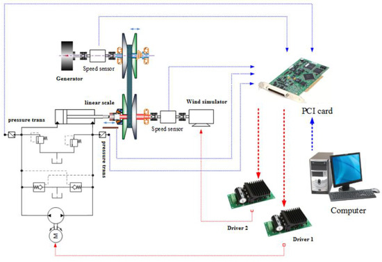
Figure 8.
Structure of experiment test rig.
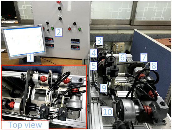
Figure 9.
Experimental apparatus: (1) program computer with Simulink; (2) control system; (3) DC motor; (4) input speed sensor; (5) primary pulley with linear encoder; (6) belt; (7) secondary pulley; (8) output speed sensor; (9) cylinder; (10) Bosch Rexroth EHA.
The EHA system is manufactured by Bosch Rexroth, which includes a gear pump, a supplementary valves system and a symmetrical double-acting cylinder and is driven by a 24V 20A DC motor. In this configuration, the movement of the cylinder is adjusted directly by the speed of the pump [21]. Two rpm sensors (SETech MS-2000) are installed in the system to measure the speed input and output of the EHA CVT. Setting parameters for the EHA system are shown in Table 1. Meanwhile, the CVT system is a customized model including a primary axis and a secondary axis. The position of the former is adjusted by the above EHA system, while that of the later is adapted passively by a spring to compromise the belt condition. The output shaft of the CVT directly drives the generator. Specification of the CVT can be found in Table 2.

Table 1.
Setting parameters for the EHA system.
Table 2.
Parameter of CVT.
The control system was implemented on a personal computer within a combination of Simulink environment and real-time Windows Target Toolbox of MATLAB. In our study, we used the ode4 (Runge–Kutta) solver in MATLAB/Simulink environment to solve several differential equations presented in Section 3 and Section 4. A multi–function data acquisition Advantech card, A/D 6014 was installed on the peripheral component interconnect (PCI) slots of the PC to perform the peripheral interfaces.
5.2. Experimental Results
For the wind turbine simulator, the rotor with a propeller radius of 3.5 m was selected to capture the wind power at an average of 10 kW. The maximum coefficient of power (Cp = 0.48) was achieved at the tip speed ratio of 8.1 and the pitch angle of the blade was 0°. To calculate the spectral power density the was assumed at 0.06 for the longitudinal components of the wind speed fluctuations and 0.2 for the lateral components.
In order to evaluate the effectiveness of the proposed WECs system, an average wind velocity of 10 m/s was investigated. From the simulation program, Figure 10 shows a plot of the wind speed and the optimal rotational input speed of the CVT with the gear box ratio 1:10. The generator power and the efficiency curve are shown in Figure 11. Based on the diagram curve, the generator needs to be tuned to an optimal speed from 220 to 280 rpm (Qingdao 10KW250RPM 240V) to achieve the highest efficiency from the output CVT speed. This is the key advantage of the proposed configuration compared with the conventional power take-off (PTO) where the speed of the generator continuously varies according to the input wind conditions [29]. As seen in these figures, the adaptive fuzzy sliding mode controller ensures an excellent tracking performance of the EHA system. After a short transition time, the tracking response adapts well with the tracking error which lies mostly in 250 rpm (Figure 12 and Figure 13). The output of angular velocity with the rotational speed setup is 250 rpm, and the response is from 230 to 270 rpm. This value is in the highest efficient region of the generator. As shown in these figures, the proposed WECs with AFSC offers the best input speed of the generator (Figure 13) compared with the conventional PID controller. The generator efficiency is around 92% with the generated power around 10.5 kW (Figure 14).
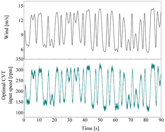
Figure 10.
Data acquisition of 10 m/s wind velocity.
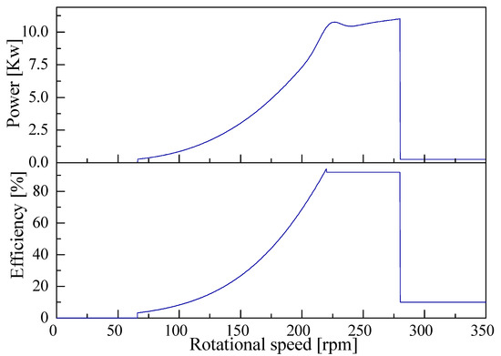
Figure 11.
Generator power and efficiency curve.
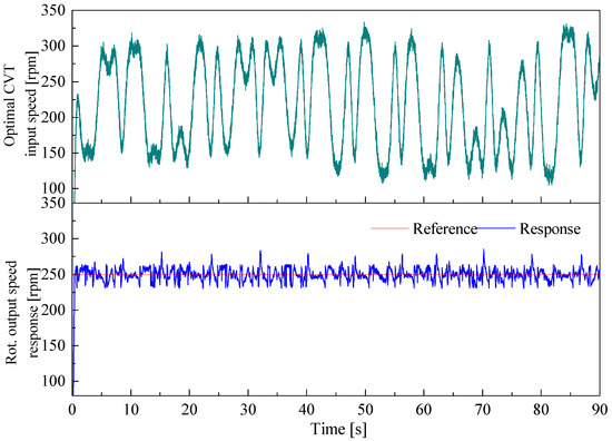
Figure 12.
CVT system response for 10 m/s wind velocity.
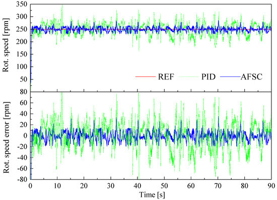
Figure 13.
Comparison between convention PID and proposed AFSC.
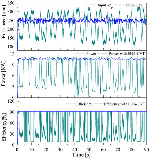
Figure 14.
Generator efficiency.
6. Conclusions
This paper presents a novel conceptual design of the power take-off system in a wind energy converter. The generator’s performance is kept at the rated speed to increase its efficiency. Here, the CVT’s ratio controlled by an EHA is employed to maintain the working speed of the generator. The adaptive fuzzy sliding mode controller is applied to control the pump of the EHA system. Experimental results indicate that the performance of the generator is smooth and stable, and the generator efficiency increased significantly. Further works involve optimizing the design parameters of the EHA CVT system as well as the propeller design before testing the prototype in real wind conditions.
Author Contributions
K.K.A. was the supervisor providing funding and administrating the project, and he reviewed and edited the manuscript. M.T.N. did the investigation, methodology, analysis, and the validation, made the MATLAB software, and wrote the original draft. T.D.D. checked the introduction, structure of the paper, reviewed and edited the manuscript. All authors contributed to this article and accepted the final report.
Funding
This research was supported by Basic Science Research Program through the National Research Foundation of Korea (NRF) funded by the Ministry of Science and ICT, South Korea (NRF2017R1A2B3004625).
Conflicts of Interest
The authors declare no conflicts of interest.
References
- Alkan, D. Investigating CVT as a Transmission System Option for Wind Turbines. Master’s Thesis, KTH School of Industrial Engineering and Management, Stockholm, Sweden, 2013. [Google Scholar]
- Jianchao, H.; Xiaolong, Z.; Pingkuo, L. A review on China’s wind power accommodation in the background of “Internet+” strategy. Int. J. Energy Res. 2018, 42, 1469–1486. [Google Scholar]
- Song, Y.; Wang, X.; Blaabjerg, F. Doubly Fed Induction Generator System Resonance Active Damping Through Stator Virtual Impedance. IEEE Trans. Ind. Electron. 2017, 64, 125–137. [Google Scholar] [CrossRef]
- Michalak, P.; Zimny, J. Wind energy development in the world, Europe and Poland from 1995 to 2009; current status and future perspectives. Renew. Sustain. Energy Rev. 2011, 15, 2330–2341. [Google Scholar] [CrossRef]
- Colak, I.; Fulli, G.; Bayhan, S.; Chondrogiannis, S.; Demirbas, S. Critical aspects of wind energy systems in smart grid applications. Renew. Sustain. Energy Rev. 2015, 52, 155–171. [Google Scholar] [CrossRef]
- Kumar, Y.; Ringenberg, J.; Depuru, S.S.; Devabhaktuni, V.K.; Lee, J.W.; Nikolaidis, E.; Andersen, B.; Afjeh, A. Wind energy: Trends and enabling technologies. Renew. Sustain. Energy Rev. 2016, 53, 209–224. [Google Scholar] [CrossRef]
- Moradi, H.; Vossoughi, G. Robust control of the variable speed wind turbines in the presence of uncertainties: A comparison between H∞ and PID controllers. Energy 2015, 90, 1508–1521. [Google Scholar] [CrossRef]
- Schulte, H.; Gauterin, E. Fault-tolerant control of wind turbines with hydrostatic transmission using Takagi–Sugeno and sliding mode techniques. Annu. Rev. Contr. 2015, 40, 82–92. [Google Scholar] [CrossRef]
- Mangialardi, L.; Mantriota, G. Continuously variable transmissions with torque-sensing regulators in waterpumping windmills. Renew. Energy 1994, 4, 807–823. [Google Scholar] [CrossRef]
- Do, H.T.; Dang, T.D.; Truong, H.V.A.; Ahn, K.K. Maximum Power Point Tracking and Output Power Control on Pressure Coupling Wind Energy Conversion System. IEEE Trans. Ind. Electron. 2018, 65, 1316–1324. [Google Scholar] [CrossRef]
- Muljadi, E.; Butterfield, C.P. Pitch-controlled variable-speed wind turbine generation. IEEE Trans. Ind. Appl. 2001, 37, 240–246. [Google Scholar] [CrossRef]
- Mohammadi, E.; Fadaeinedjad, R.; Naji, H.R. Flicker emission, voltage fluctuations, and mechanical loads for small-scale stall-and yaw-controlled wind turbines. Energy Conv. Manag. 2018, 165, 567–577. [Google Scholar] [CrossRef]
- Mangialardi, L.; Mantriota, G. Automatically Regulated CVT in Wind Power-Systems. Renew. Energy 1994, 4, 299–310. [Google Scholar]
- Ehtiwesh, I.A.S.; Dorovic, Z. Comparative analysis of different control strategies for electro-hydraulic servo systems. Proc. World Acad. Sci. Eng. Tech. 2009, 56, 906–909. [Google Scholar]
- Nguyen, M.T.; Dang, X.B.; Ahn, K.K. A Gain-Adaptive Intelligent Nonlinear Control for an Electrohydraulic Rotary Actuator. Int. J. Precis. Eng. Manuf. 2018, 19, 665–673. [Google Scholar]
- Jun, L.; Yongling, F.; Guiying, Z.; Bo, G.; Jiming, M. Research on fast response and high accuracy control of an airborne brushless DC motor. In Proceedings of the IEEE International Conference on Robotics and Biomimetics, Shenyang, China, 22–26 August 2004; pp. 807–810. [Google Scholar]
- Truong, D.Q.; Ahn, K.K. Force control for press machines using an online smart tuning fuzzy PID based on a robust extended Kalman filter. Expert Syst. Appl. 2011, 38, 5879–5894. [Google Scholar] [CrossRef]
- Lin, Y.; Shi, Y.; Burton, R. Modeling and robust discrete-time sliding-mode control design for a fluid power electrohydraulic actuator (EHA) system. IEEE/ASME Trans. Mech. 2013, 18, 1–10. [Google Scholar] [CrossRef]
- Perron, M.; de Lafontaine, J.; Desjardins, Y. Sliding-mode control of a servomotor-pump in a position control application. In Proceedings of the Canadian Conference on Electrical and Computer Engineering, Saskatoon, SK, Canada, 1–4 May 2005; pp. 1287–1291. [Google Scholar]
- Ahn, K.K.; Nam, D.N.C.; Jin, M. Adaptive backstepping control of an electrohydraulic actuator. IEEE/ASME Trans. Mech. 2014, 19, 987–995. [Google Scholar] [CrossRef]
- Nguyen, M.T.; Doan, N.C.N.; Park, H.G.; Ahn, K.K. Trajectory control of an electro hydraulic actuator using an iterative backstepping control scheme. Mechatronics 2015, 29, 96–102. [Google Scholar]
- Choi, B.J.; Kwak, S.W.; Kim, B.K. Design of a single-input fuzzy logic controller and its properties. Fuzzy Sets Syst. 1999, 106, 299–308. [Google Scholar] [CrossRef]
- Wang, L.X. Adaptive Fuzzy Systems and Control: Design and Stability Analysis; Englewood Cliffs: New York, NY, USA, 1994. [Google Scholar]
- Lee, H.; Tomizuka, M. Robust adaptive control using a universal approximator for SISO nonlinear systems. IEEE Trans. Fuzzy Syst. 2000, 8, 95–106. [Google Scholar]
- Do, H.T.; Ahn, K.K. Velocity control of a secondary controlled closed-loop hydrostatic transmission system using an adaptive fuzzy sliding mode controller. J. Mech. Sci. Tech. 2013, 27, 875–884. [Google Scholar] [CrossRef]
- Do, H.T.; Park, H.G.; Ahn, K.K. Application of an adaptive fuzzy sliding mode controller in velocity control of a secondary controlled hydrostatic transmission system. Mechatronics 2014, 24, 1157–1165. [Google Scholar] [CrossRef]
- Chiang, M.H.; Lee, L.W.; Liu, H.H. Adaptive fuzzy sliding-mode control for variable displacement hydraulic servo system. In Proceedings of the IEEE International Fuzzy Systems Conference, London, UK, 23–26 July 2007; pp. 1–6. [Google Scholar]
- Noroozi, N.; Roopaei, M.; Jahromi, M.Z. Adaptive fuzzy sliding mode control scheme for uncertain systems. Commun. Nonlinear Sci. Numer. Simul. 2009, 14, 3978–3992. [Google Scholar] [CrossRef]
- Nguyen, M.T.; Phan, C.B.; Ahn, K.K. Power Take-Off System Based on Continuously Variable Transmission Configuration for Wave Energy Converter. Int. J. Precis. Eng. Manuf. Green Tech. 2018, 5, 89–101. [Google Scholar]
- Naidu, N.K.S.; Singh, B. Sensorless control of single voltage source converter-based doubly fed induction generator for variable speed wind energy conversion system. IET Power Electron. 2014, 7, 2996–3006. [Google Scholar] [CrossRef]
- Carlin, P.W.; Laxson, A.S.; Muljadi, E.B. The History and State of the Art of Variable-Speed Wind Turbine Technology. Wind Power 2003, 6, 129–159. [Google Scholar] [CrossRef]
- Simanaitis, D. CVTs are coming of age. Road Track 2004, 5, 122–124. [Google Scholar]
- Kim, P.; Ryu, W.; Kim, H.; Hwang, S.; Kim, H. A study on the reduction in pressure fluctuations for an independent pressure-control-type continuously variable transmission. Proc. Inst. Mech. Eng. Part D J. Auto. Eng. 2008, 222, 729–737. [Google Scholar] [CrossRef]
- Le, T.D.; Bui, N.M.T.; Ahn, K.K. Improvement of Vibration Isolation Performance of Isolation System Using Negative Stiffness Structure. IEEE/ASME Trans. Mech. 2016, 21, 1561–1571. [Google Scholar] [CrossRef]
© 2019 by the authors. Licensee MDPI, Basel, Switzerland. This article is an open access article distributed under the terms and conditions of the Creative Commons Attribution (CC BY) license (http://creativecommons.org/licenses/by/4.0/).