Partial Discharge Classification Using Deep Learning Methods—Survey of Recent Progress

1
Ormazabal Corporate Technology, 48340 Amorebieta, Spain
2
Department of Electronic Engineering and Communications, University of Zaragoza, 50018 Zaragoza, Spain
3
Instituto CIRCE (Universidad de Zaragoza—Fundación CIRCE), 50018 Zaragoza, Spain
*
Author to whom correspondence should be addressed.
Energies 2019, 12(13), 2485; https://doi.org/10.3390/en12132485
Submission received: 28 May 2019
/
Revised: 19 June 2019
/
Accepted: 27 June 2019
/
Published: 27 June 2019
(This article belongs to the Special Issue Application of Machine Learning and Data Mining in Electrical Engineering)
Abstract
:This paper examines the recent advances made in the field of Deep Learning (DL) methods for the automated identification of Partial Discharges (PD). PD activity is an indication of the state and operational conditions of electrical equipment systems. There are several techniques for on-line PD measurements, but the typical classification and recognition method is made off-line and involves an expert manually extracting appropriate features from raw data and then using these to diagnose PD type and severity. Many methods have been developed over the years, so that the appropriate features expertly extracted are used as input for Machine Learning (ML) algorithms. More recently, with the developments in computation and data storage, DL methods have been used for automated features extraction and classification. Several contributions have demonstrated that Deep Neural Networks (DNN) have better accuracy than the typical ML methods providing more efficient automated identification techniques. However, improvements could be made regarding the general applicability of the method, the data acquisition, and the optimal DNN structure.
1. Introduction
Efficient fault diagnosis is crucial to prevent costly outages of electrical network systems. Nowadays, with the increasing presence of smart grid technologies, Smart Diagnosis implementation using more automated techniques must also be considered. Partial Discharges (PD) measurements and analysis is widely used as a diagnostic indicator of insulation deterioration in electrical equipment such as, transformers, rotating machines, medium voltage cables, gas insulated switchgear (GIS) [1,2]. PD can be defined as a localized dielectric breakdown of a small portion of a solid or liquid electrical insulation system under high voltage stress and can lead to total insulation failure.
Over the years, in order to automate classification of PD fault sources, several algorithms have been developed. The most efficient were those with Machine Learning (ML), but this was only a semi-automated classification because the input data has to be previously given by the user, who must have knowledge about which features are important for the algorithm, and as such includes a lot of bias. Raymond et al. [3] presented a review including different techniques for feature extraction and the PD classification methods used by different authors. Furthermore, Mas’ud et al. [4] investigated the application of conventional Artificial Neural Networks (ANN) for PD classification through a literature survey. Nowadays, with the developments in computation and data storage, interest is focused on automated features extraction and classification by Deep Learning (DL) algorithms with Deep Neural Networks (DNN), where the expert is not so necessary. Therefore, this paper examines the recent advances made on the application of DNN techniques for PD source recognition.
Deep Learning is a subfield of Machine Learning, which is also a subset of the Artificial Intelligence field, as shown in Figure 1. ML uses algorithms to parse data, learn from that data, and make informed decisions based on what they have learned, but usually they need some manual feature engineering, as illustrated at the top-right of Figure 1. On the other hand, the DL algorithms are based on ANNs built by many layers and nodes that can learn and make intelligent decisions or predictions on their own, including automatic feature extraction. This concept is described at the bottom-right of Figure 1.
2. Partial Discharge Background
According to the IEC-60270 [5] a PD is “a localized electrical discharge that only partially bridges the insulation between conductors and which can or cannot occur adjacent to a conductor.” The detection of this discharge gives an indication of the state of insulation of equipment, the proper identification of which can help to find the real source of this defect. When the PD phenomenon occurs, it results in an extremely fast transient current pulse with a rise time and pulse width that depends on the discharge type or defect type. Several electrical and electromagnetic methods are used to measure this electromagnetic wave at very high frequencies. According to IEC TS 62478 [6] the ranges are usually HF from 3 to 30 MHz, VHF from 30 to 300 MHz and UHF between 300 MHz and 3 GHz.
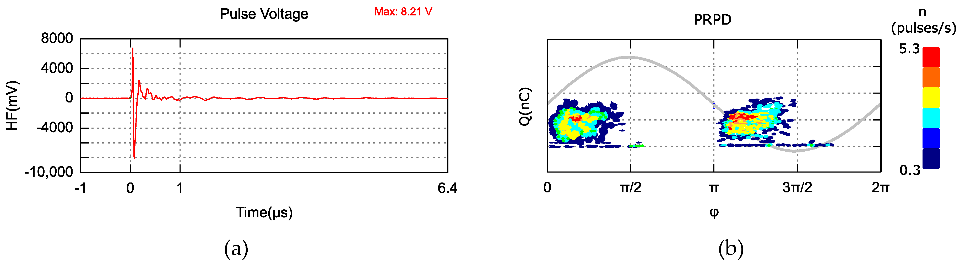
The PD is measured by sensors based on capacitive, inductive and electromagnetic detection principles or near-field antennas. The output signals from the sensor are damped oscillating pulses of high frequency and can be represented in the time-domain as an individual PD pulse waveform as shown in Figure 2a. The phase-resolved PD (PRPD) pattern is widely used to characterize this phenomenon and represents the apparent charge (Q) versus the corresponding phase angle at which the PD occurs (φ) in the AC network voltage, and their rates of occurrence (n) within a specified time interval Δt. An example of PRPD is shown in Figure 2b.
A strong correlation exists between these PD representations and the nature of PD sources (defects); thereby a recognition (or classification) could be made extracting discriminatory features from these representations. From the PRPD pattern, statistical parameters can calculated (skewness, kurtosis, mean, variance and cross correlation) [7]. There are also some image processing tools: texture analysis algorithms, fractal features, wavelet-based image decomposition, which can be applied to extract informative features from the PRPD image. Alternatively, with signal processing tools such as Fourier series analysis, Haar and Walsh transforms or wavelet transform, the features can be obtained from the time-domain representation [8]. However, all these techniques provide semi-automatic feature extraction and a lot of effort and expertise is required. Therefore, the implementation of DNN techniques that implies automated features extraction and classification is preferred and is discussed in next sections.
3. Deep Neural Network (DNN)
The use of the “deep” term started in 2006, after G. Hinton et al. published a paper [9] showing how to train a DNN. Any ANN with more than two hidden layers may be considered as deep.
For a better understanding of the use of these techniques for PD classification, some DNN models will be presented in this section.
3.1. Recurrent Neural Network (RNN)
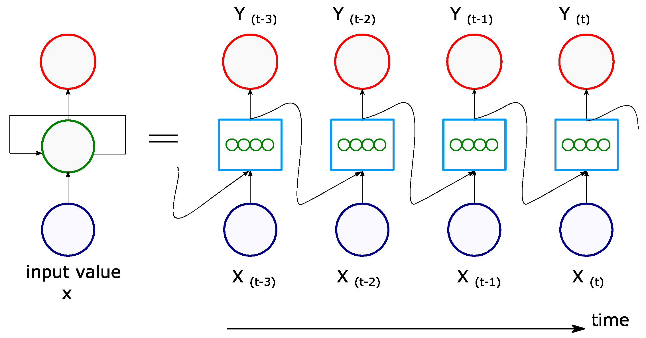
This model includes feedback connections intended to analyze and predict time series data. A representation of a simple Recurrent Neural Network (RNN) architecture is shown to the left of Figure 3, with one hidden layer receiving inputs, producing an output, and sending that output back to itself. If the RNN representation is expanded in a temporal frame as shown on the right of Figure 3, at each time step this recurrent layer receives the inputs as well as its own outputs from the previous time step,
In an RNN structure, the neuron has two sets of weights assigned: for the inputs and for the outputs of the previous time step:. The mathematical formulation of this neuron process can be written as Equation (1).
The main characteristic of RNN is that recurrent neurons have a short-term memory of the previous state. Moreover, the DNN structures may suffer from the vanishing gradients problem, that is, when updates from Gradient Descent leave the layer connection weights virtually unchanged for initial inputs when time series are very long, and training does not converge to a suitable solution. As an alternative to this problem, a neural network layer that preserves some state across time steps, called a memory cell can be used. Various types of memory cells with long-term memory have been introduced and the most popular is the Long Short-Term Memory model (LSTM) [10].
3.2. Autoencoders (AEs)
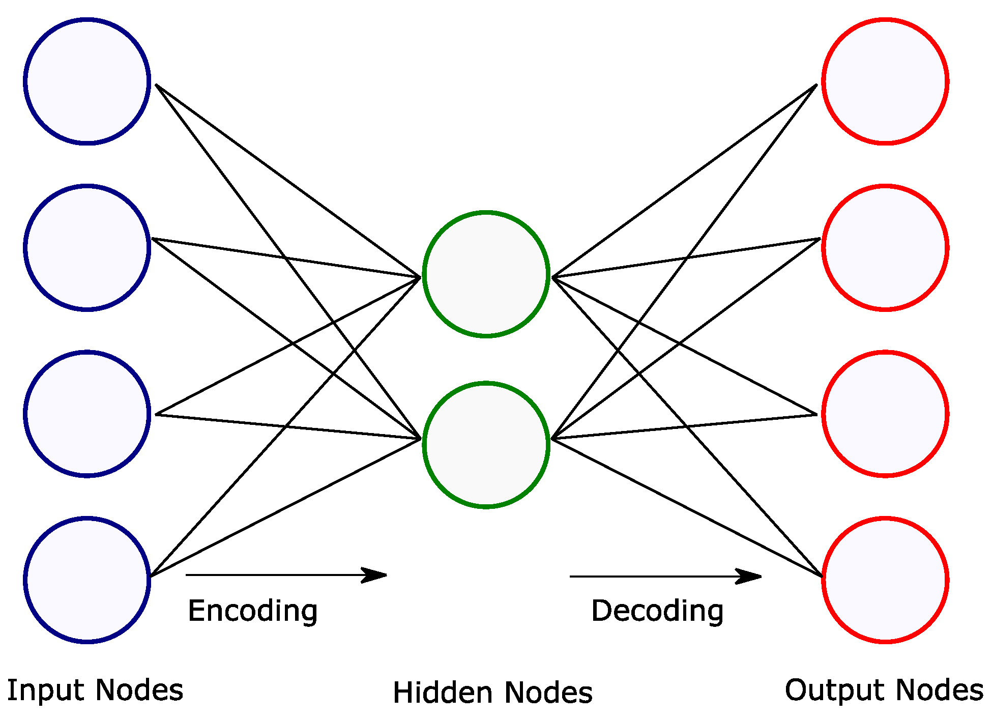
These kinds of models are considered as unsupervised learning models (or self-supervised), being able to generate efficient representation of the input data (feature extraction). The aim of autoencoders (AEs) is to output a replication of its inputs, therefore, the outputs are often called reconstruction, and its cost function contains a recognition loss that penalizes the model when the reconstructions are different from the inputs. In this architecture, the numbers of neurons in the output layer must be equal to the number of inputs. The encoding part converts the inputs to an internal representation and the decoding part converts this internal representation to the outputs, as is shown in Figure 4.
AEs are useful for data dimensionality reduction when the hidden layer has fewer nodes than the inputs, and act as a powerful feature extractor [11]. Therefore, to extract more features, more nodes have to be added into the hidden layer, but this could be a problem when training the AE if the number of hidden neurons is larger than the optimum number of features. In this case, some hidden nodes could just monopolize the activation and make other neurons unused. A typical solution to this problem is a Sparse AE, which can manage more nodes in the hidden layer than inputs, by forcing the generation of a sparse encoding during the training phase (where most output activations are null). When AEs have multiple hidden layers they are called Stacked AE or deep autoencoders.
The autoencoder also behaves as a generative model; they are capable of generating new data from the input data that are very similar to this original set.
3.3. Generative Adversarial Networks (GANs)
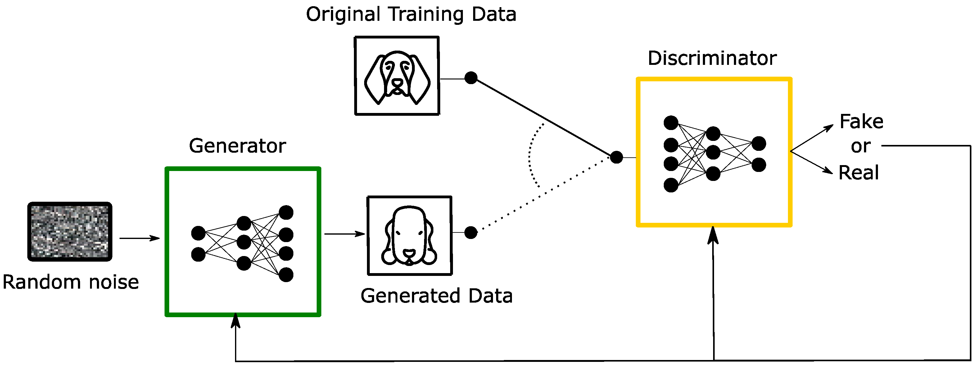
Generative Adversarial Networks (GAN) is a truly generative model proposed in 2014 [12]. The GAN architecture, shown in Figure 5, is composed of two different stages, represented by two neural networks: the generator network and the discriminator network. The generator tries to emulate data that comes from some probability distribution, usually processing a random input called latent representation. The discriminator estimates the probability that a sample came from the real data or from the generator. The training ends when the discriminator is no longer able to differentiate between the real and the fake data, and the generator network can be used to generate new simulated data.
3.4. Convolutional Neural Network (CNN)
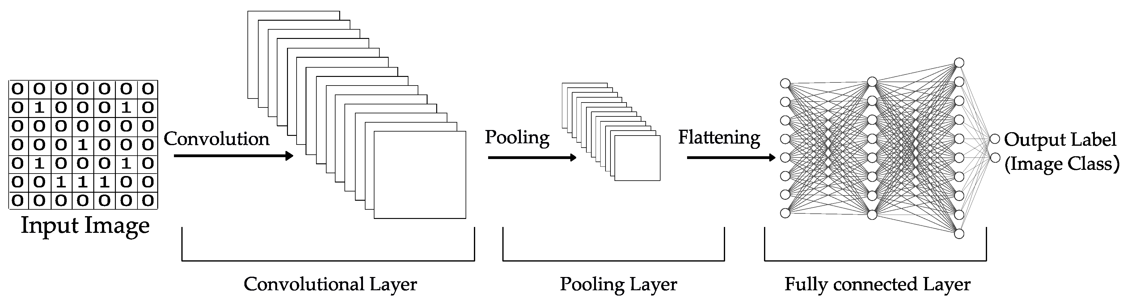
Convolutional Neural Networks (CNNs) are inspired by the brain’s visual cortex but are not restricted to visual perception; they are also successful with signal processing and recognition. The principal task of image classification is to obtain a class or a probability of classes that best describes the input image. To perform this task, the algorithm has to be able to recognize features (edges, curves, ridges) and their compositions [13]. A basic CNN architecture is shown in Figure 6, whose basic layers are:
- Convolutional layer: in this layer each filter (also called Kernel) is applied to the image in successive positions along the image and through convolution operations, generates a features map.
- Nonlinear layer: a non-linear activation function, such as ReLu (Rectified Linear Unit) function, is used to avoid linearity in the system.
- Pooling (down-sampling) layer: the aim of this layer is to reduce the computational load by reducing the size of the feature maps, and also introduces positional invariance.
- Fully connected layers: ANN that takes the convolutional features (previously flattened) generated by the last convolutional layer and makes a prediction (e.g., softmax function). The output error is established by the loss function to inform how accurate the network is, and finally use an optimizer to increase its effectiveness.
4. Partial Discharges Classification with DNN
In order to investigate the application of DNN for PD classification and recognition, a review of recent progress is made in this section and it will be organized according to the type of DNN structure and the PD data used as inputs in several recent papers. At the end of this section a table will summarize the findings.
4.1. Simple DNN Structure
PRPD Data
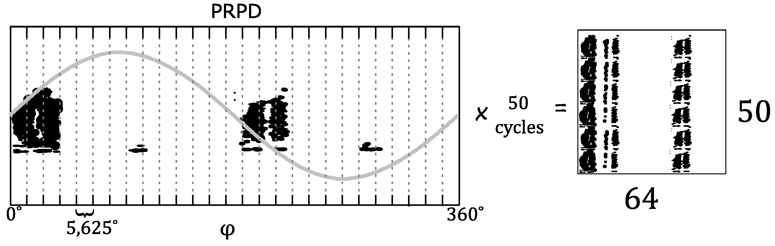
The first DNN applied for PD diagnosis was proposed by Catterson and Sheng in 2015 [14]. Their objective was to classify six different PD defects constructed in oil: (1) bad electrical contact, (2) floating potential, (3) and (4) metallic protrusion in two different configurations, (5) free particle and (6) surface discharge. They recorded approximately 250–300 PRPD patterns, measured with a UHF sensor, but since this quantity is not enough for training the DNN, a data augmentation phase was applied to have over 1000 examples for each defect type. The PRPD pattern was generated after one second (50 AC cycles) with a phase window of 5.625°, that can be represented as a 50 × 64 pixel image, shown in Figure 7, giving 3200 pixel values that represents the relative PD amplitude recorded. These values are used as input for the network.
Firstly, they searched the optimal quantity of neurons in one hidden layer of a conventional ANN structure, finding good accuracy starting at 75 neurons and overall peak at 3000 neurons. Then a DNN architecture including hidden layers with 100 neurons was explored varying from one to seven layers, concluding that five hidden layers are an appropriate number. They also made a comparison between two different activation functions: ReLu and sigmoid function. They found that accuracy can be increased from 72% (one hidden layer—ANN) up to 86% (five hidden layers—DNN) with ReLu activation function. Even though a simple DNN structure was proposed in this paper, the interesting results stimulated other researchers to investigate more complex DNN structures and their application in PD detection and classification.
4.2. Recurrent Neural Network (RNN)
4.2.1. PRPD Data
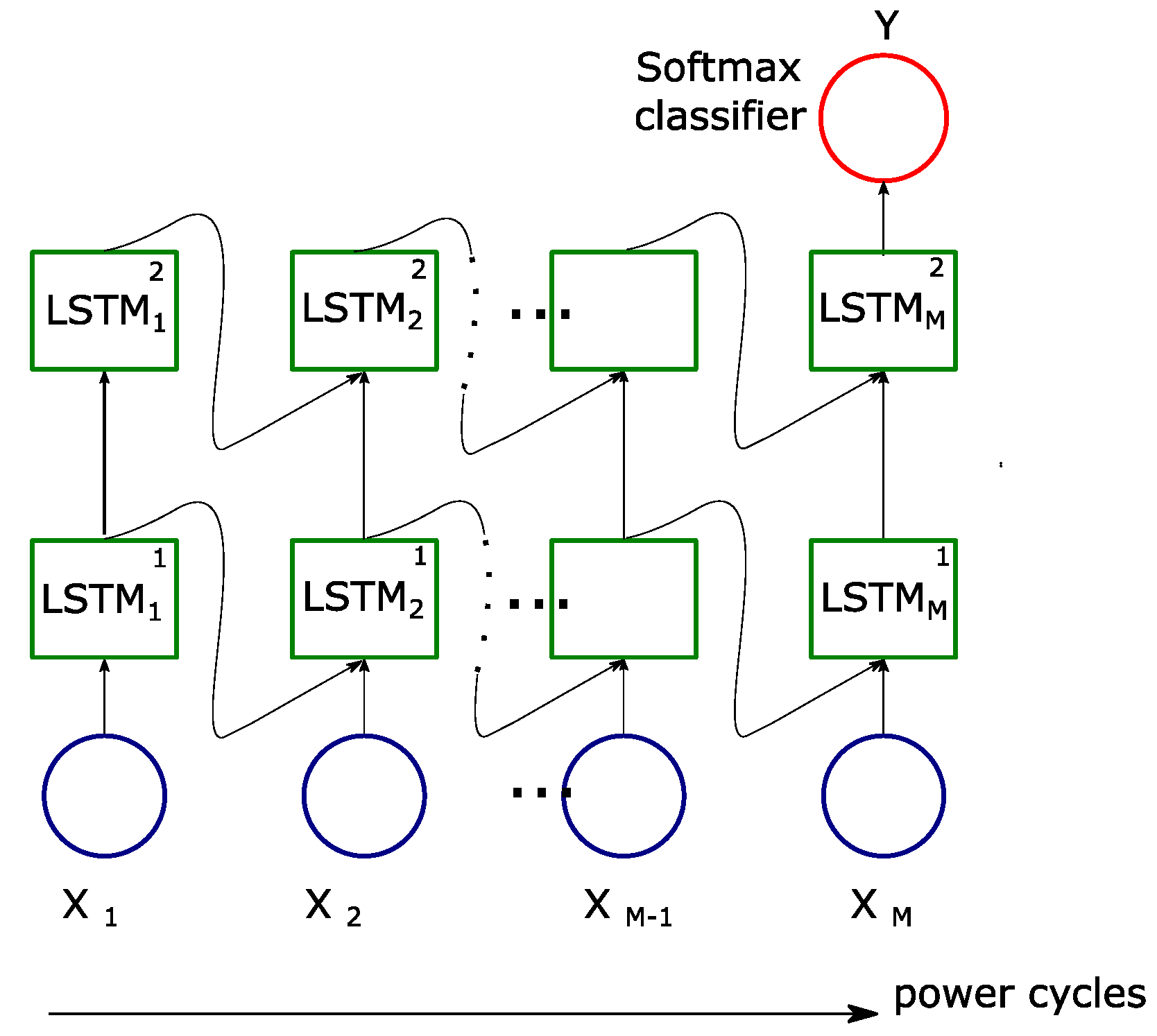
The first RNN structure with LSTM layers was proposed by Nguyen et al. [15] with an Adam optimization algorithm to train the model and an early stopping technique to prevent overfitting. Finally, a softmax layer was used to classify four different PD sources and an artificial noise source. As in the research explained above, the PD sources (corona, floating, free particle and void defect) were artificially generated with pre-constructed cells installed in a 345 kV GIS chamber experimental setup in the laboratory. However, the data set they obtained in the experiments is imbalanced, i.e., data obtained from the experiments are not uniformly distributed across the different classes, the void defect class has 242 experiments, on the other hand, the floating defect class only 35, this could be a problem if is not well addressed [16,17], because the class distribution forces the classification algorithms to be biased to the majority class and the features of the minority class are not adequately learned.
The input data is a vector containing 128 data points with information from the PRPD in one power cycle in the -th cycle, i.e., each cycle considered is a time step of this network establishing thus the temporal dependencies. To find the optimal performance of the network they evaluated it for a different number of power cycles and LSTM layers, finding that for power cycles and two LSTM layers the accuracy model reached 96.62%. This model, shown in Figure 8, also outperforms other techniques: Linear Support Vector Machine (SVM) (88.63%), Non Linear SVM (90.71%), and a conventional ANN (93.01%).
4.2.2. Time-Series Data
Adam and Tenbohlen [18] also proposed a LSTM network, where the input data is a single PD signal waveform. The PD signals were obtained from four different artificial sources measured in the laboratory. The data set consisted of 42,794 recorded impulses, and even though the classes were not balanced, they found that using all of them improves accuracy more than reducing the data to balance classes. They found that this classification based on single PD pulses is feasible and accurate and could be an alternative to using PRPD data, in which patterns vary if two PD sources are present at the same time. Despite the fact that sensors could acquire a single pulse, being the combination of two pulses produced by two different sources, the two PD phenomena occur at different times and would still be possible to detect separate pulses within one power cycle.
4.3. Autoencoder
4.3.1. PRPD Data
An autoencoder structure was proposed by Tang et al. [19], more precisely a stacked sparse auto-encoder (SSAE) to train the hidden layers that will extract meaningful features from the PRPD data. A softmax output layer was used to classify PD in four severity stages: (1) Normal, (2) Attention, (3) Serious and (4) Dangerous stage. A Fuzzy-C means clustering (FCM) algorithm was previously used to categorize the raw data in those stages. The data were collected from experimental cells that simulate four different PD defect types in a GIS enclosure: (a) protrusion defect, (b) particle defect, (c) contamination defect and (d) gap defect. The UHF PD signals were acquired with an antenna and they obtained a PRPD representation for each PD type at different voltages to represent its development (from the initial discharge stage and increasing gradually to the breakdown). The input data consisted of 2000 samples for each voltage value.
Additionally, nine statistical features were calculated to be used as input for an SVM algorithm and compared with the SSAE method.
Table 1 shows the recognition average accuracy for the four defects, and it is clearly seen how the SSAE method is more accurate for all cases.
4.3.2. Features Extracted from PRPD and Raw Signal Data
In [20] an autoencoder was used to classify five artificial defects manufactured on a cable in the laboratory, and in [21] a Deep Belief Network (DBN) was trained to recognize internal, surface and corona PDs recreated in a laboratory environment. Even though it was demonstrated that those DNN models have better accuracy than other machine learning techniques (e.g., Decision tree, Kernel Fisher Discriminant Analysis and SVM), characteristics were manually extracted from the raw data to use as input data, when the interest in using DNNs is the automatic feature extraction.
4.4. Convolutional Neural Network (CNN)
4.4.1. Waveform Spectrogram Data
Lu et al. [22] proposed a CNN with five layers, 500 nodes per layer, ReLu activation functions and a softmax output function. Their aim was to detect PD signals within different noise and interference signals. Measurements in switchgear were recorded using a Transient Earth voltage (TEV) method, as sound clips, and then transformed into an image represented by time-frequency spectra. White noise, impulse noise, and periodic noise spectra were also presented. Altogether, the CNN was trained with 3000 images containing 500 PD signals. The network´s accuracy was compared with other detection methods actually used for PD detection, summarized in Table 2, and shows that CNN was the most accurate in classifying the different PD sources and noises. Although, the CNN and the pulse current method have similar detection rate, the CNN needs less time to perform the detection. The ultrasonic method has the lowest detection rate because it can solely detect surface discharges and not internal discharges.
These results suggest that the use of a CNN structure allows PD detection more efficiently and faster than the other existing techniques used in this work. However, more information is needed about the specific CNN used and how it was trained. Moreover, the images used as the CNN input as spectral representation should be more specific to know if this image physically represents the PD phenomenon.
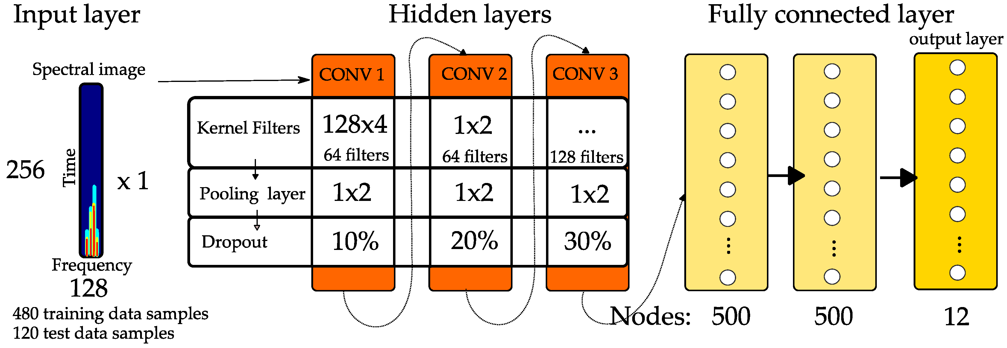
A detailed CNN structure was presented by Li et al. [23] and is schematically shown in Figure 9. As inputs, they also use a spectral image, consisting of 256 time bins and 128 frequency bins, obtained by the Short Time Fourier Transform (STFT) applied to the recorded UHF PD signal, explaining the procedure and showing the time-frequency scale considered. The filters used in the convolutional layer are one dimensional, applied on the frequency axis.
The PD signals were obtained by a simulation model using a Finite-Difference Time-Domain (FDTD) method and the aim of the CNN was to classify 12 different kinds of PD sources in a 120 kV GIS model. The total data set for the training was 600 images. They obtained a 100% performance with the CNN method and they compared it with an SVM classifier, where input features were calculated by advanced signal processing methods such as Hilbert-Huang Transform (91.7% accuracy) and Wavelet Transform (96.7% accuracy).
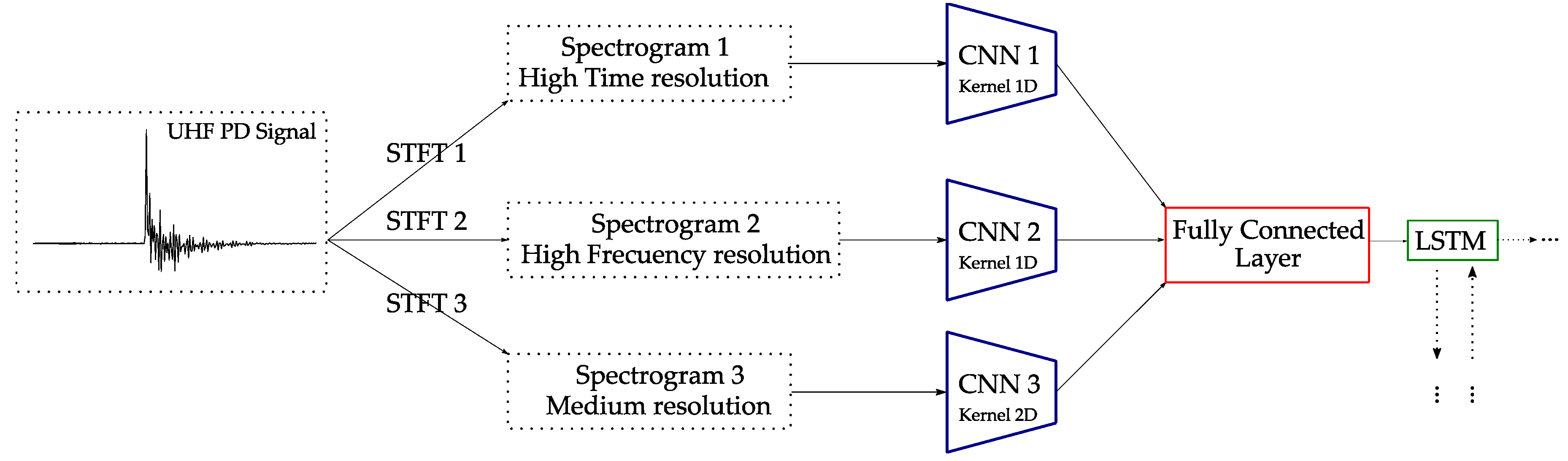
Years later, the same authors published another CNN architecture combined with a LSTM network [24]. In this case, for each UHF signal they calculate three different STFTs considering different window lengths to represent the signal in three types of spectrograms: (a) high time resolution, (b) high frequency resolution and (c) medium resolution. These three spectrograms separately are used as input for three different subnetworks (CNNs with different filters) and combined at the end by a fully connected layer. The model decides which filter or subnetwork gives a more comprehensive representation of the original signal. Finally, this information is merged in a LSTM module. The structure proposed is shown in Figure 10.
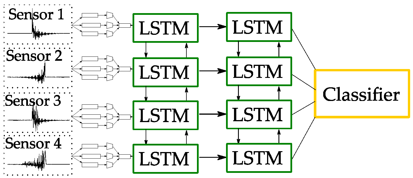
The LSTM network, as shown in Figure 11, is used to integrate information from signals recorded by sensors installed in four different positions away from the PD source. With this scheme it is possible to consider the signal attenuation when it is propagated in the system. Five types of PD were generated in a GIS tank model in a laboratory environment. The overall identification accuracy was 98.2% and comparison was made in scenarios with a single sensor and a single spectrogram representation.
4.4.2. Time-Domain Waveform Data
Dey et al. [25] also used a CNN structure to classify impulse-fault patterns in transformers, but it could also be applied to PD pattern classification. The input data for this CNN structure was time-series data instead of an image and it was tested for single and multiple faults (i.e., simultaneously occurring at two different winding locations). The faults are created in an analogous model of a 33 kV winding of a 3 MVA transformer (based on a real life model) and they investigated the applicability issues of the method on a real transformer, with unknown design, simulating the model in an EMTP environment (Electromagnetic Transient Programming), finding that the performance decreased from 91.1% to 80% when the basic parameter values of the transformer winding changed by 15%. Nevertheless, this method outperforms, by more than 7% on average, other existing techniques, for example self-organizing maps, fuzzy logic and SVM.
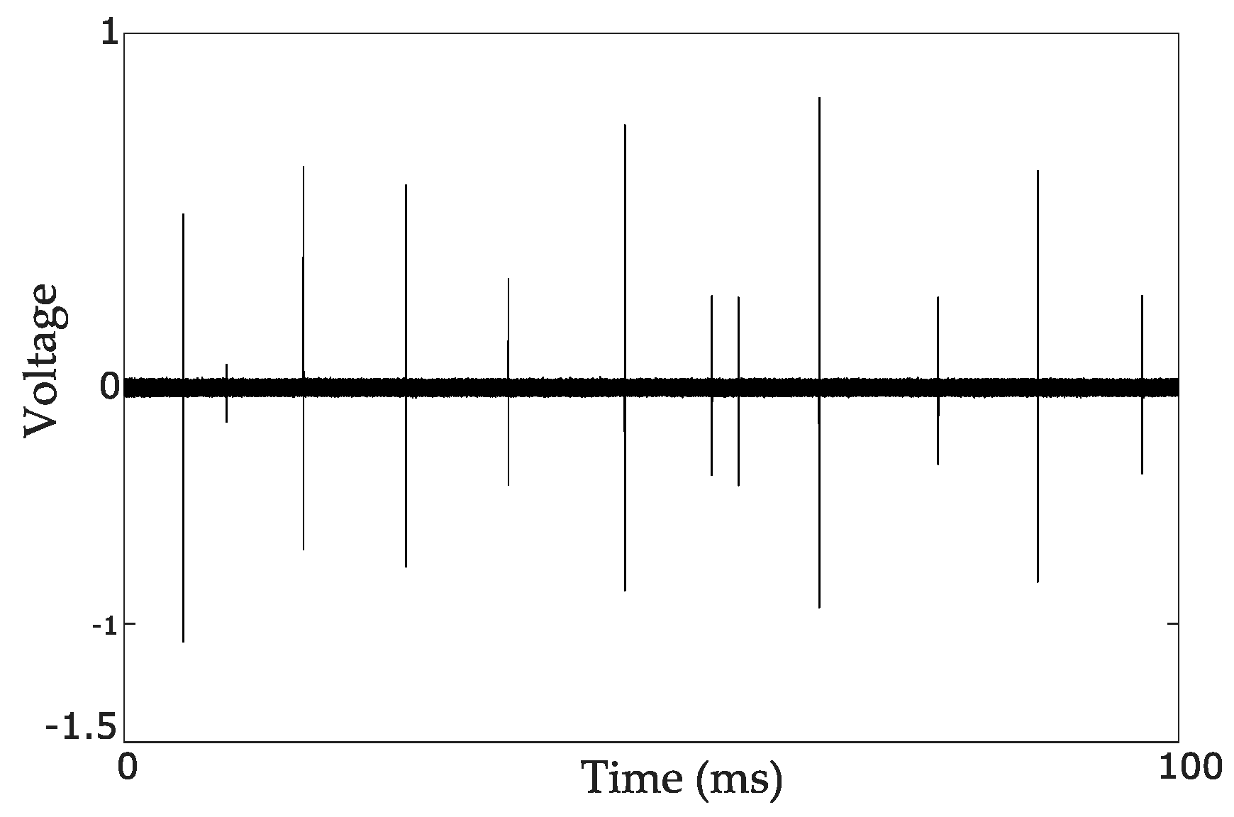
The authors in [26] use TEV signals recorded from two artificial PD sources measured in a laboratory. As input for the CNN, they use a time-domain waveform image of the signals recorded over 100 ms (five consecutive power cycles). The data was previously preprocessed in four different steps, and they investigated which step was the most important for a correct classification. An example of raw PD data recorded in this interval of time is shown in Figure 12. To demonstrate the practical use of this technique, data from a real PD source is also used for training, but it represents only 4% of all data, and this amount may not be sufficiently representative. The first hidden layer of this CNN structure convolves 64 filters of 5 × 1, followed by a max pooling layer of 2 × 1. The second hidden layer is similar to the first hidden layer with a dropout rate of 0.5; the dropout layer randomly annuls a fraction of the outputs forcing the layer representation to be more distributed. The output layer consists of a fully connected layer followed by a softmax classifier. The cross entropy cost function is used for training.
A similar representation to that shown in Figure 12 is also used in [27]. The data set is collected from on-site and simulation experiments using UHF sensors. The authors introduce a new approach for the CNN structure, using a one dimensional CNN, that differs from the previous ones in the size of convolution and pooling kernels, being 1-D arrays instead of 2-D matrices. The accuracy of this model was 85% and was higher compared with SVM and a conventional ANN. A comparison of this 1-D model with a conventional 2-D CNN suggests that the computation time can be reduced using this less complex model.
4.4.3. PRPD Data
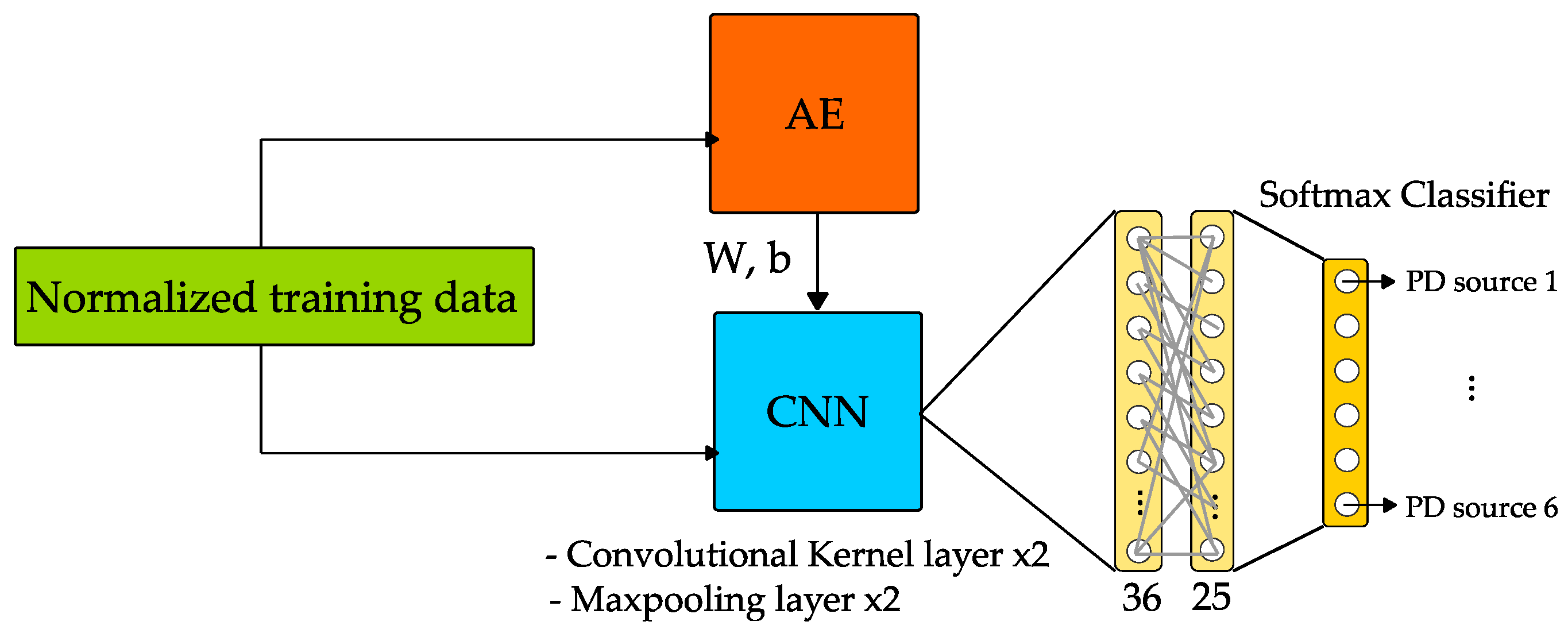
An Autoencoder was used by Song et al. [28] to generate preliminary features from the PD test data and the network layers were used to initialize parameters of the convolutional layers in a CNN (transfer learning technique). The authors used a CNN structure which is composed of two convolutional layers, two pooling layers, two fully connected layers and the output layer with a softmax output function, as schematically shown in Figure 13. The classification task was to identify six different PD sources.
A more complex data collection is presented in this paper, obtained by on-site substation detection and laboratory experiments with different detection instruments and UHF sensors. For the experimental part, five PD sources simulated with cells were implemented in a GIS: (1) floating electrode, (2) surface, (3) corona, (4) insulation void and (5) free metal particle discharge. Interference patterns were also recorded. The data is recorded as PRPD data in 50 power cycles, with a phase window of 5° (phase dimension: 360°/5° = 72), and the amplitude is linearly normalized according to the maximum and minimum values of the sample data. Therefore, the input data for training is normalized and represented as a 72 × 50 matrix. For the training task, data sets with 1000 examples were prepared.
Training with 800 random data samples, the performance of this DNN model is 89.7% and is compared with others classification techniques using classical statistical features. The accuracy for the SVM technique was 79.3%, and 72.4% for a conventional ANN, showing that the DNN can extract more meaningful features to represent the PD phenomena and to classify them accurately.
They also investigate the influence of the training data using only laboratory experimental data and then a mix of half set of on-site substation detection and half set of experimental data. The results are shown in Table 3. The recognition accuracy decreases for all methods when the data from substations is used, but the DNN still presents a higher robustness. These results highlight the problem of the method applicability when the network is trained with modeled defects that do not represent PDs in a real environment.
4.4.4. Features Extracted from Raw Signal Data
A comparison between CNN, RNN and DNN models was made in [29], resulting in a CNN being more accurate than a RNN structure. Nevertheless, the details of the model structures were not clearly explained. The data set was obtained from a PD simulator by an ultrasonic sensor, but the input data could be considered as features manually extracted from the UHF signal, because, after down-sampling the ultrasonic sample to obtain a sound that humans can hear, sound feature extraction methods were applied. To train a CNN model, the input data has to be a structured data set (like an image) and the 193 features extracted from different methods used in this work are not.
4.5. Generative Adversarial Networks (GANs)
Time-Domain Waveform Data
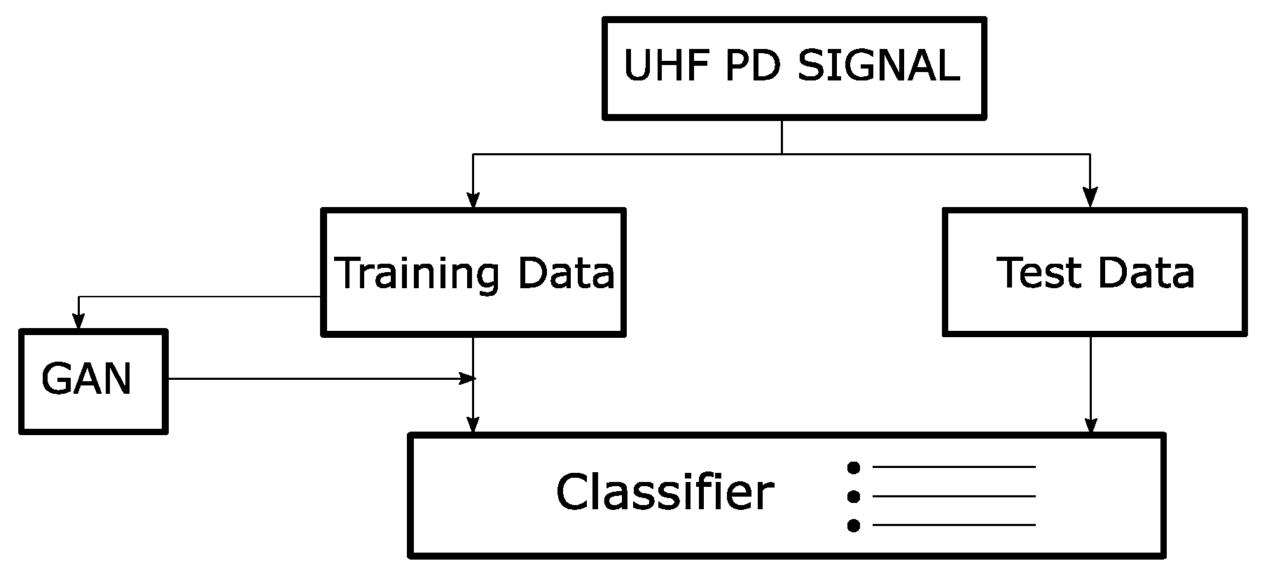
Generative Adversarial Network (GAN) models were used to obtain more PD data by data augmentation since sometimes it is hard and expensive to gather enough data to correctly train a DNN and prevent overfitting of the model. Wang et al. [30] used this model to enlarge the UHF PD signals obtained from PD simulator experiments. To classify three PD sources an ANN was trained with real data and fake generated data provided for the GAN, and finally tested only with real data, and the proposed scheme is shown in Figure 14. Results demonstrated that the classification accuracy is better when the model is trained with the same number of real and fake data and starts to decrease when fake data is larger than the real data. In [31] a GAN model also was used to generate more data from experimental PD sources made in a cable, but features were extracted from the raw signal data.
A summary of the methods that were explained in this section is shown in Table 4.
5. Discussion
After this literature review on the application of DNN for partial discharge recognition or/and classification, it was found that these techniques are more accurate than the usual machine learning techniques, mainly because the PD raw data can be provided to the deep neural network without previous manual feature extraction, so it automatically learns which are the most representative features of each type of PD. However, most of these models were trained with data from artificial PD sources constructed in laboratories and with few real samples; this could be an issue in their application in real electrical installations. Indeed, the accuracy in the recognition will depend on the reliability of the training data. If these data do not represent exactly the same phenomenon found in real installations, the DNN will not make a reasonable prediction. Although these data have successfully been used for a preliminary approach, building a database of real PD sources in electrical installations and measured with different sensor technologies would be the first step to make this technique practical and efficient.
The Convolutional Neural Network (CNN) is the most applicable model; the input data for this network needs to be an image or a signal with relevant structural information, such as time-series data. Many authors have used the PRPD as input data, but apart from the time it takes to obtain this image pattern regularity depends on the PD development over time, the state of the insulation at time of measurement, applied voltage, recording time and the acquisition sensor used. A more ideal concept would be to use the raw pulses registered by the sensor, as some authors have done, using a single pulse waveform or several consecutives pulses recorded over time, or transforming the pulses into a spectrogram image. Other representations could also be investigated to avoid limitations imposed by the STFT in the spectrogram representation, as the Local Polynomial Fourier Transform [32] or a scalogram [33].
Most authors have presented the results of a single neural network, but deep learning neural networks are nonlinear methods that learn via a stochastic training algorithm, and with each training process may find a different set of weights, which in turn produce different predictions. A better approach would be to use an ensemble learning, to reduce the variance of DNN models by training multiple models instead of a single model and to combine the predictions from these models. Moreover, other approaches could be also considered such as repeating experiments and providing statistics on different learnings, sensitivity analysis, ablation studies, etc.
The application of the DNN techniques in real electrical environments was not found in the literature; therefore, an industrial application interest is discussed in next section.
Potential Industrial Interest and Application of PD Recognition Based on DNN Techniques
The accurate localization of a partial discharge source can reduce the response time for a maintenance team dramatically. In terms of partial discharges in cables, the pinpointing of a PD source to within a few meters equates to a maintenance team being able to go directly to the place and excavate a small area. Within the substation environment, a PD source could be more difficult to localize, and as such, the identification of PD type is useful.
There are systems available on the market for the detection and measurement of PD sources. However, these systems tend to be expensive and often require interruption in service for installation and measurement. Nowadays, in a smart grid context, on-line techniques are more suitable, and utilities are working alongside manufacturers to develop more affordable monitoring solutions. Smart condition monitoring is the key solution to diagnose equipment incipient failure, and this requires intelligent algorithms to extract meaningful information from raw data, make predictions and provide accurate, real-time asset health insights. Therefore, deep learning methods could be an excellent option for these requirements.
The automatic identification of PD sources online using an attractive techno-economically optimized system based on deep learning methods, which is possible with the ongoing advancement of GPUs (graphics processing units) for embedded applications and algorithms written in freely available programming languages such as Python or R, is an attractive option for network operators, maintenance providers and also brings added value to equipment manufacturer’s products.
6. Conclusions
In this paper a descriptive summary about the recent advances made in the field of Deep Learning methods for the automated identification of PD activity was presented. The focus was on the PD data input used to train the DNNs because this is the main component of the method’s general applicability. Few research papers that use PD data acquired in the field were found. Most data used was obtained from experiments in the laboratory or from simulations that could lead to a lack of generality, and the method would not be applicable to measurements made in real installations. Moreover, research has to be made to find the optimal PD data representation useful for training the DNN that implies less time-consuming recording and reduction in data storage.
Within the DNN architectures used, the CNN model is the most often applied, which was shown to achieve a great success for image recognition. The combination of two models was also found in the literature, for example, a CNN combined with an Autoencoder or with an LSTM model. Although, they demonstrated to be more accurate than the conventional Machine Learning techniques, the optimal DNN structure and its implementation applicability for smart diagnosis in the smart grid have yet to be discovered.
Author Contributions
S.B. wrote the original draft manuscript; S.B. and D.B. provided the literature analysis for the review article. D.B. provided theoretical guidance of the method; I.G., D.B. and M.P.C. reviewed and edited the paper manuscript; I.G. provided industrial application guidance of the method; I.O. and M.P.C. supervized and supported this research.
Funding
This project received funding from the European Union’s Horizon 2020 research and innovation programme under the Marie Sklodowska-Curie grant agreement No 676042.
Conflicts of Interest
The authors declare no conflict of interest.
References
- Montanari, G.C.; Cavallini, A. Partial discharge diagnostics: from apparatus monitoring to smart grid assessment. IEEE Electr. Insul. Mag. 2013, 29, 8–17. [Google Scholar] [CrossRef]
- Stone, G.C. Partial discharge diagnostics and electrical equipment insulation condition assessment. IEEE Trans. Dielectr. Electr. Insul. 2005, 12, 891–904. [Google Scholar] [CrossRef]
- Raymond, W.J.K.; Illias, H.A.; Bakar, A.H.A.; Mokhlis, H. Partial discharge classifications: Review of recent progress. Measurement 2015, 68, 164–181. [Google Scholar] [CrossRef] [Green Version]
- Mas’ud, A.; Albarracín, R.; Ardila-Rey, J.; Muhammad-Sukki, F.; Illias, H.; Bani, N.; Munir, A. Artificial Neural Network Application for Partial Discharge Recognition: Survey and Future Directions. Energies 2016, 9, 574. [Google Scholar] [CrossRef]
- Internationale Elektrotechnische Kommission. High-Voltage Test Techniques—Partial Discharge Measurements =: Techniques des essais à haute tension—mesures des décharges partielles; International Electrotechnical Commission Central Office: Geneva, Switzerland, 2015; ISBN 978-2-8322-3053-4. [Google Scholar]
- Internationale Elektrotechnische Kommission. High Voltage Test Techniques—Measurement of Partial Discharges by Electromagnetic and Acoustic Methods: Technical Specification = Techniques d’essais à haute tension—mesurage des décharges partielles par méthodes électromagnétiques et acoustiques; Specification Technique; International Electrotechnical Commission Central Office: Geneva, Switzerland, 2016; ISBN 978-2-8322-3560-7. [Google Scholar]
- Gulski, E.; Kreuger, F.H. Computer-aided recognition of discharge sources. IEEE Trans. Electr. Insul. 1992, 27, 82–92. [Google Scholar] [CrossRef]
- Sahoo, N.C.; Salama, M.M.A.; Bartnikas, R. Trends in partial discharge pattern classification: A survey. IEEE Trans. Dielectr. Electr. Insul. 2005, 12, 248–264. [Google Scholar] [CrossRef]
- Hinton, G.E.; Osindero, S.; Teh, Y.-W. A Fast Learning Algorithm for Deep Belief Nets. Neural Comput. 2006, 18, 1527–1554. [Google Scholar] [CrossRef] [PubMed]
- Hochreiter, S.; Schmidhuber, J. Long Short-Term Memory. Neural Comput. 1997, 9, 1735–1780. [Google Scholar] [CrossRef] [PubMed]
- Vincent, P.; Larochelle, H.; Bengio, Y.; Manzagol, P.-A. Extracting and composing robust features with denoising autoencoders. In Proceedings of the 25th international conference on Machine learning—ICML ’08, Helsinki, Finland, 5–9 July 2008; ACM Press: Helsinki, Finland, 2008; pp. 1096–1103. [Google Scholar] [Green Version]
- Goodfellow, I.; Pouget-Abadie, J.; Mirza, M.; Xu, B.; Warde-Farley, D.; Ozair, S.; Courville, A.; Bengio, Y. Generative Adversarial Nets. In Advances in Neural Information Processing Systems 27; Ghahramani, Z., Welling, M., Cortes, C., Lawrence, N.D., Weinberger, K.Q., Eds.; Curran Associates, Inc.: Dutchess County, NY, USA, 2014; pp. 2672–2680. [Google Scholar]
- LeCun, Y.; Kavukcuoglu, K.; Farabet, C. Convolutional networks and applications in vision. In Proceedings of the 2010 IEEE International Symposium on Circuits and Systems, Paris, France, 30 May–2 June 2010; pp. 253–256. [Google Scholar]
- Catterson, V.M.; Sheng, B. Deep neural networks for understanding and diagnosing partial discharge data. In Proceedings of the 2015 IEEE Electrical Insulation Conference (EIC), Seattle, WA, USA, 7–10 June 2015; pp. 218–221. [Google Scholar]
- Nguyen, M.-T.; Nguyen, V.-H.; Yun, S.-J.; Kim, Y.-H. Recurrent Neural Network for Partial Discharge Diagnosis in Gas-Insulated Switchgear. Energies 2018, 11, 1202. [Google Scholar] [CrossRef]
- Wang, S.; Liu, W.; Wu, J.; Cao, L.; Meng, Q.; Kennedy, P.J. Training deep neural networks on imbalanced data sets. In Proceedings of the 2016 International Joint Conference on Neural Networks (IJCNN), Vancouver, BC, Canada, 24–29 July 2016; pp. 4368–4374. [Google Scholar]
- Yan, Y.; Chen, M.; Shyu, M.; Chen, S. Deep Learning for Imbalanced Multimedia Data Classification. In Proceedings of the 2015 IEEE International Symposium on Multimedia (ISM), Miami, FL, USA, 14–16 December 2015; pp. 483–488. [Google Scholar]
- Adam, B.; Tenbohlen, S. Classification of multiple PD Sources by Signal Features and LSTM Networks. In Proceedings of the 2018 IEEE International Conference on High Voltage Engineering and Application (ICHVE), ATHENS, Greece, 10–13 September 2018; pp. 1–4. [Google Scholar]
- Tang, J.; Jin, M.; Zeng, F.; Zhang, X.; Huang, R. Assessment of PD severity in gas-insulated switchgear with an SSAE. IET Sci. Meas. Technol. 2017, 11, 423–430. [Google Scholar] [CrossRef]
- Wang, G.; Yang, F.; Peng, X.; Wu, Y.; Liu, T.; Li, Z. Partial Discharge Pattern Recognition of High Voltage Cables Based on the Stacked Denoising Autoencoder Method. In Proceedings of the 2018 International Conference on Power System Technology (POWERCON), Guangzhou, China, 6–8 November 2018; pp. 3778–3792. [Google Scholar]
- Karimi, M.; Majidi, M.; Etezadi-Amoli, M.; Oskuoee, M. Partial Discharge Classification Using Deep Belief Networks. In Proceedings of the 2018 IEEE/PES Transmission and Distribution Conference and Exposition (T&D), Denver, CO, USA, 16–19 April 2018; pp. 1061–1070. [Google Scholar]
- Lu, Y.; Wei, R.; Chen, J.; Yuan, J. Convolutional Neural Network Based Transient Earth Voltage Detection. In Proceedings of the 2016 15th International Symposium on Parallel and Distributed Computing (ISPDC), Fuzhou, China, 8–10 July 2016; pp. 386–389. [Google Scholar]
- Li, G.; Rong, M.; Wang, X.; Li, X.; Li, Y. Partial discharge patterns recognition with deep Convolutional Neural Networks. In Proceedings of the 2016 International Conference on Condition Monitoring and Diagnosis (CMD), Xi’an, China, 25–28 September 2016; pp. 324–327. [Google Scholar]
- Li, G.; Wang, X.; Li, X.; Yang, A.; Rong, M. Partial Discharge Recognition with a Multi-Resolution Convolutional Neural Network. Sensors 2018, 18, 3512. [Google Scholar] [CrossRef] [PubMed]
- Dey, D.; Chatterjee, B.; Dalai, S.; Munshi, S.; Chakravorti, S. A deep learning framework using convolution neural network for classification of impulse fault patterns in transformers with increased accuracy. IEEE Trans. Dielectr. Electr. Insul. 2017, 24, 3894–3897. [Google Scholar] [CrossRef]
- Banno, K.; Nakamura, Y.; Fujii, Y.; Takano, T. Partial Discharge Source Classification for Switchgears with Transient Earth Voltage Sensor Using Convolutional Neural Network. In Proceedings of the 2018 Condition Monitoring and Diagnosis (CMD), Perth, WA, Australia, 23–26 September 2018; pp. 1–5. [Google Scholar]
- Wan, X.; Song, H.; Luo, L.; Li, Z.; Sheng, G.; Jiang, X. Pattern Recognition of Partial Discharge Image Based on One-dimensional Convolutional Neural Network. In Proceedings of the 2018 Condition Monitoring and Diagnosis (CMD), Perth, WA, Australia, 23–26 September 2018; pp. 1–4. [Google Scholar]
- Song, H.; Dai, J.; Sheng, G.; Jiang, X. GIS partial discharge pattern recognition via deep convolutional neural network under complex data source. IEEE Trans. Dielectr. Electr. Insul. 2018, 25, 678–685. [Google Scholar] [CrossRef]
- Zhang, Q.; Lin, J.; Song, H.; Sheng, G. Fault Identification Based on PD Ultrasonic Signal Using RNN, DNN and CNN. In Proceedings of the 2018 Condition Monitoring and Diagnosis (CMD), Perth, WA, Australia, 23–26 September 2018; pp. 1–6. [Google Scholar]
- Wang, X.; Huang, H.; Hu, Y.; Yang, Y. Partial Discharge Pattern Recognition with Data Augmentation based on Generative Adversarial Networks. In Proceedings of the 2018 Condition Monitoring and Diagnosis (CMD), Perth, WA, Australia, 23–26 September 2018; pp. 1–4. [Google Scholar]
- Wu, Y.; Lu, C.; Wang, G.; Peng, X.; Liu, T.; Zhao, Y. Partial Discharge Data Augmentation of High Voltage Cables based on the Variable Noise Superposition and Generative Adversarial Network. In Proceedings of the 2018 International Conference on Power System Technology (POWERCON), Guangzhou, China, 6–8 November 2018; pp. 3855–3859. [Google Scholar]
- Rojas, H.E.; Forero, M.C.; Cortes, C.A. Application of the local polynomial Fourier transform in the evaluation of electrical signals generated by partial discharges in distribution transformers. IEEE Trans. Dielectr. Electr. Insul. 2017, 24, 227–236. [Google Scholar] [CrossRef]
- Ren, Z.; Qian, K.; Wang, Y.; Zhang, Z.; Pandit, V.; Baird, A.; Schuller, B. Deep Scalogram Representations for Acoustic Scene Classification. IEEE/CAA J. Autom. Sin. 2018, 5, 662–669. [Google Scholar] [CrossRef]
Figure 1.
Relationship between Artificial Intelligence, Machine Learning and Deep Learning.
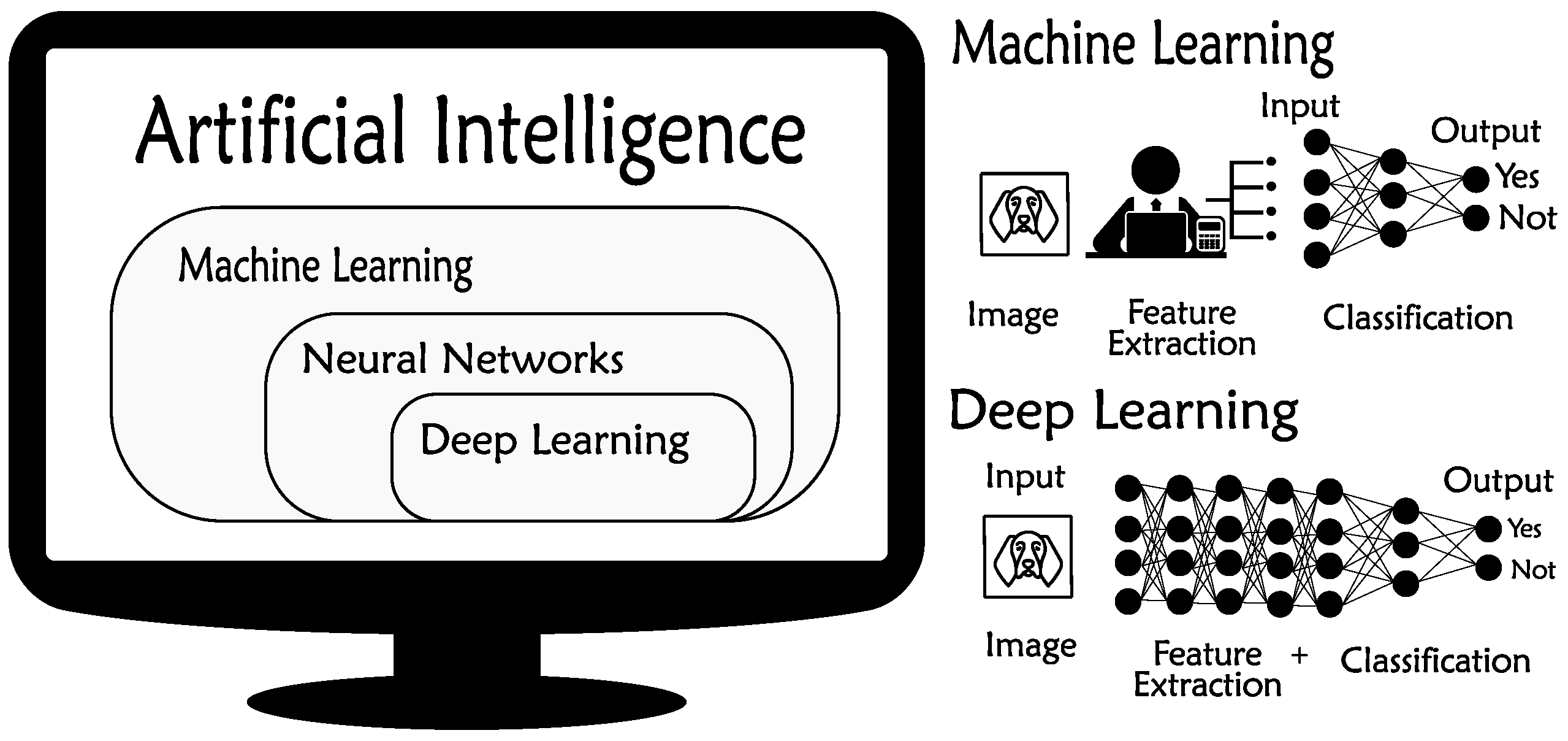
Figure 2.
Partial discharge representations; (a) Partial Discharge (PD) waveform in time-domain. (b) Phase resolved Partial Discharge (PRPD) Pattern.
Figure 2.
Partial discharge representations; (a) Partial Discharge (PD) waveform in time-domain. (b) Phase resolved Partial Discharge (PRPD) Pattern.

Figure 3.
Example of a simple Recurrent Neural Network (RNN) architecture.

Figure 4.
Simple autoencoder architecture with one hidden layer.

Figure 5.
Generative Adversarial Network Architecture.

Figure 6.
Convolutional Neural Network Architecture.

Figure 7.
PRPD data used as input data for the Deep Neural Network (DNN), adapted from [14].
Figure 7.
PRPD data used as input data for the Deep Neural Network (DNN), adapted from [14].

Figure 8.
RNN structure with Long Short-Term Memory model (LSTM) layers proposed by Nguyen et al. [15].
Figure 8.
RNN structure with Long Short-Term Memory model (LSTM) layers proposed by Nguyen et al. [15].

Figure 9.
CNN structure proposed by [23] used to classify PD spectrograms.
Figure 9.
CNN structure proposed by [23] used to classify PD spectrograms.

Figure 10.
CNN subnetworks proposed by [24] with different input data representation of the UHF PD signal.
Figure 10.
CNN subnetworks proposed by [24] with different input data representation of the UHF PD signal.

Figure 11.
Multi-resolution CNN and LSTM fusion structure proposed by [24].
Figure 11.
Multi-resolution CNN and LSTM fusion structure proposed by [24].

Figure 12.
Image representation of a raw PD data recorded in five power cycles.

Figure 13.
CNN structure combined with an autoencoder (AE) model proposed by [28].
Figure 13.
CNN structure combined with an autoencoder (AE) model proposed by [28].

Figure 14.
Classification of PD sources using a Generative Adversarial Network (GAN) model to generate more training data samples, adapted from [30].
Figure 14.
Classification of PD sources using a Generative Adversarial Network (GAN) model to generate more training data samples, adapted from [30].


Table 1.
Average recognition accuracy results comparison between stacked sparse auto-encoder (SSAE) model and Support Vector Machine (SVM) technique.
Table 1.
Average recognition accuracy results comparison between stacked sparse auto-encoder (SSAE) model and Support Vector Machine (SVM) technique.
| Defect | SSAE (%) | SVM (%) |
|---|---|---|
| Protrusion | 88 | 77 |
| Particle | 93 | 81 |
| Contamination | 88 | 80 |
| Gap | 90 | 83 |
Table 2.
Results comparison between Convolutional Neural Networks (CNN) and traditional methods.
| Methods | PD Detection Rate (%) | Recognition Accuracy (%) | Detection Time Cost |
|---|---|---|---|
| CNN | 95.73 | 95.58 | 12 s |
| Pulse Current | 95.36 | 90.81 | >30 min |
| Ultrasonic | 48.10 | 85.73 | ≈ 5 min |
| Existing TEV | 80.68 | 80.90 | ≈ 10 min |
Table 3.
Overall average accuracy comparison of training data.
| Model | Only Experimental Data (%) | Mixed Data (%) |
|---|---|---|
| CNN | 95.6 | 86.7 |
| SVM | 91.5 | 74.2 |
| ANN | 90.6 | 70.2 |
Table 4.
Summary of DNN techniques that have been used for PD classification.
| DNN Structure | Input Data | N° PD Sources | Origin of Sources | Sensor | Reference | Year |
|---|---|---|---|---|---|---|
| DNN | PRPD | 6 | Artificial PDs constructed in oil | UHF | Catterson and Sheng [14] | 2015 |
| RNN LSTM | PRPD | 4 | Experimental PD cells in GIS | UHF | Nguyen et al. [15] | 2018 |
| Time-Domain Waveform | 4 | Artificial PDs created in laboratory | According to IEC 60270 | Adam and Tenbohlen [18] | 2018 | |
| AE | PRPD | 4 | Experimental PD cells in GIS | UHF | Tang et al. [19] | 2017 |
| Features from signal | 5 | Artificial PDs in cables | According to IEC 60270 | Wang et al. [20] | 2018 | |
| DBN | Features from PRPD | 17 | Artificial PDs created in laboratory | HF | Karimi et al. [21] | 2018 |
| CNN | Waveform Spectrogram | 2 | High Voltage Switchgears | TEV | Lu et al. [22] | 2016 |
| 12 | Simulation with FDTD method | UHF | Li et al. [23] | 2016 | ||
| CNN + LSTM | 5 | Artificial PDs in GIS tank | UHF | Li et al. [24] | 2018 | |
| CNN | Time-Domain Waveform | 5 | - | - | Dey et al. [25] | 2017 |
| Time-Domain Waveform Image | 2 | Artificial PDs created in laboratory and real PD in transformer | TEV | Banno et al. [26] | 2018 | |
| 5 | On-site detection and simulations experiments | UHF | Wan et al. [27] | 2018 | ||
| CNN + AE | PRPD | 6 | Experimental PD cells in GIS and real PD in substation | UHF | Song et al. [28] | 2018 |
| CNN RNN DNN | Features from signal | 6 | PD simulator | UHF | Zhang et al. [29] | 2018 |
| GAN | Features from signal | 5 | Artificial PDs in cables | According to IEC 60270 | Wu et al. [31] | 2018 |
| Time-Domain Waveform | 3 | PD simulator | UHF | Wang et al. [30] | 2018 |
© 2019 by the authors. Licensee MDPI, Basel, Switzerland. This article is an open access article distributed under the terms and conditions of the Creative Commons Attribution (CC BY) license (http://creativecommons.org/licenses/by/4.0/).
Share and Cite
MDPI and ACS Style
Barrios, S.; Buldain, D.; Comech, M.P.; Gilbert, I.; Orue, I. Partial Discharge Classification Using Deep Learning Methods—Survey of Recent Progress. Energies 2019, 12, 2485. https://doi.org/10.3390/en12132485
AMA Style
Barrios S, Buldain D, Comech MP, Gilbert I, Orue I. Partial Discharge Classification Using Deep Learning Methods—Survey of Recent Progress. Energies. 2019; 12(13):2485. https://doi.org/10.3390/en12132485
Chicago/Turabian StyleBarrios, Sonia, David Buldain, María Paz Comech, Ian Gilbert, and Iñaki Orue. 2019. "Partial Discharge Classification Using Deep Learning Methods—Survey of Recent Progress" Energies 12, no. 13: 2485. https://doi.org/10.3390/en12132485
Note that from the first issue of 2016, this journal uses article numbers instead of page numbers. See further details here.