Increasing the Competitiveness of Tidal Systems by Means of the Improvement of Installation and Maintenance Maneuvers in First Generation Tidal Energy Converters—An Economic Argumentation

Abstract

The most important technological advances in tidal systems are currently taking place in first generation tidal energy converters (TECs), which are installed in areas in which the depth does not exceed 40 m. Some of these devices are fixed to the seabed and it is, therefore, necessary to have special high performance ships to transport them from the base port to the tidal farm and to subsequently recover the main units of these devices. These ships are very costly, thus making the installation costs very high and, in some cases, probably unfeasible. According to what has occurred to date, the costs of the installation and maintenance procedures depend, to a great extent, on the reliability and accessibility of the devices. One of the possible solutions as regards increasing system performance and decreasing the costs of the installation and maintenance procedures is the definition of automated maneuvers, which will consequently influence: (i) an increase in the competitiveness of these technologies; (ii) a reduction in the number and duration of installation and maintenance operations; (iii) less human intervention, or (iv) the possibility of using cheaper general purpose ships rather than high cost special vessels for maintenance purposes, among others. In this research, we propose a definition of the procedures required for the manual and automated installation and maintenance maneuvers of gravity-based first generation TECs. This definition will allow us to quantify the costs of both the manual and automated operations in a more accurate manner and enable us to determine the reduction in the cost of the automated installation and maintenance procedures. It will also enable us to demonstrate that the automation of these maneuvers may be an interesting solution by which to improve the competitiveness of tidal systems in the near future.

1. Introduction

The large-scale exploitation of fossil fuels has had important environmental repercussions such as climate change or the rise in sea level amongst others [1,2]. This means that there is currently a need to reduce the dependence on fossil fuels and place greater emphasis on renewable energy sources in order to fulfil future sustainable energy needs [3,4]. In 2009, the European Union (EU) established that 20% of final energy consumption should originate from renewable sources by 2020 [5], and additionally set 2050 as the target year by which emissions will have been reduced by 80% [6,7]. In this context, and with the aim of achieving a sustainable development, in 2015, the United Nations Framework Convention on Climate Change was established in order to reduce the causes of climate change as regards food production and limit the increase in temperature (increases of up to 1.5 $°$C) [8]. A number of viable renewable energies could, therefore, be exploited to achieve this goal, among which marine renewable energy (MRE) is attracting increased attention [9].

MRE is currently recognized as being an abundant, geographically diverse energy resource that has both the public’s acceptance and positive associated externalities (economic growth, job creation or the mitigation of the negative impacts of climate change, etc.) [10]. It can be exploited from offshore wind, waves, tides, tidal currents, thermal gradients or salinity gradients. This paper is focused on the exploitation of the tidal current resource, which it is hoped will play a major role in meeting future energy needs with regard to other renewable energy sources thanks to its high predictability, stability and high load factor [11]. If we wish to employ technologies to harness the energy obtained from tidal currents in order to attain sustainable development, it is necessary to use natural resources in an efficient manner, i.e., we must optimize their exploitation [12]. Devices that can be utilized to harness tidal current power where the depth is no greater than 40 m have been developed by various technology manufacturers [13,14]. These devices, which are denominated as first generation tidal energy converters (TECs), are normally supported on bases that are fastened to the seabed by means of various types of anchoring systems (monopole, piloted or gravity). It is undoubtedly technically feasible to employ these devices to harness energy from tidal currents, although very few tidal stream projects are currently operating at a commercial stage [15]. This is principally owing to the fact that it typically costs more to generate energy from tidal currents than it does when using other renewable technologies [16]. It is consequently vital to understand the parameters that may affect the cost structure in order to provide a framework containing areas in which these costs can be reduced [17].

A detailed analysis of the life cycle costs (LCC) for first generation tidal energy farms (TEFs) shows that the installation and maintenance procedures are of the utmost importance and must be optimized in order to increase their current potential, help their acceleration and sustainability and help attract investment in these technologies [18,19]. These procedures include the transportation of each of the TECs from the base port to its installation site, the preparation of the seabed, the placement and installation of anchor systems and/or the deployment of a mooring system, and the positioning, connection and disconnection of the main units of the devices [20,21]. These tasks necessitate the use of special high-performance ships that are equipped with dynamic positioning, large cranes, etc., and this implies high installation and maintenance costs [22,23]. The installation and maintenance costs are greatly dependent upon the accessibility and reliability of the device [16]. It would, however, be possible to increase system performance and decrease the aforementioned costs by automating the performance of the immersion and emersion maneuvers [24,25]. This can be done by controlling the ballast water inside the devices, which consequently permits the implementation of a closed loop depth and/or orientation control that makes(s) it possible to: (i) raise the generation unit from the seabed to the surface of the sea and (ii) carry out the same operation but in reverse. We can perform these automatic maneuvers by using small guide wires and by controlling the ballast water inside the device. The achievement of this objective will consequently influence: (i) less human intervention, (ii) the possibility of using the cheapest general purpose ships rather than high cost special vessels for maintenance purposes, (iii) a reduction in the number and duration of installation and maintenance operations or (iv) an increase in the competitiveness of these technologies, among others. The potential benefits of these systems are very important, but, as they are in an early stage of development, studies that address the economic feasibility of these systems have not yet been developed. Several authors have produced interesting papers comprising feasibility studies concerning other types of offshore projects. These include: wind energy [26], wave energy [27], co-located projects (wind and wave energy) [28] and hybrid projects (wind and wave energy) [29]. No economic-financial studies focusing on the automation of installation and maintenance maneuvers have, however, been produced to date.

The main contributions of this research are the following: (i) we discuss the merits of automated installation and maintenance maneuvers with regard to manual maneuvers for an idealized gravity (a substantial mass is used to support the structure on which the TEC is placed.) -based first generation TEC designed by our research group (Grupo de Investigación Tecnológico en Energías Renovables Marinas, GIT-ERM); (ii) we provide interesting information about manual and automated installation and operation maneuvers for these tidal energy technologies, which is not usually found in scientific literature as these technologies are at an initial (pre-commercial) stage of development, and (iii) we carry out a comparative economic-financial feasibility study for these maneuvers, which illustrates that the development of advanced automation systems for these maneuvers may be a very interesting approach by which to increase the competitiveness of this source of renewable energy in the near future.

The remainder of the paper is organized as follows: Section 2 describes the procedures used to carry out installation and maintenance maneuvers for first generation TECs in both a manual and an automated fashion. The procedure used to evaluate the economic-financial feasibility of tidal energy projects using manual or automated maneuvers is briefly explained in Section 3. Section 4 shows the results attained after carrying out a numerical case study of a 50 MW TEF in the cases of both manual and automated maneuvers. Finally, Section 5 is devoted to our conclusions and proposals for future works.

2. Description of Installation and Maintenance Maneuvers for Gravity-Based First Generation TECs

In this section, we provide details on the installation and maintenance maneuvers for gravity-based first generation TECs. It should be noted that the information regarding these sorts of maneuvers is very limited owing to the fact that these technologies are currently at an initial stage of development (pre-commercial stage), signifying that real data about these maneuvers is not yet available [30]. The implementation of improved procedures for installation and maintenance maneuvers will actively influence their successful future commercialization [31], and this is one of the most important aspects studied by the GIT-ERM research group. The vessels used to perform these maneuvers should have the following characteristics: (i) Dynamic positioning, which allows redundancy in order to ensure work under extreme conditions and to guarantee security and reliability while these maneuvers are being carried out. These kinds of vessels have a high level of technology and are very costly to acquire/rent [32,33]; (ii) a Heavy lifting crane. Any cranes operating with these gravity-based first generation TECs must have a lifting capacity of around 250 tons [34], and (iii) the special vessel needs to have a high area on its deck on which to transport the structure, gondolas, auxiliary tools, etc. The aforementioned considerations allow us to conclude that the characteristics of the vessels required to carry out these maneuvers are not typical since the number of specialized vessels is not currently high and they are not easy to find on the market. They are, at present, used in the installation and maintenance of offshore wind energy farms and in the oil and gas industry, but the cost of hiring them is currently very high and oscillates according to the market (thus causing a high economic dependence). Furthermore, other sorts of vessels, such as remotely operated vehicles (ROVs), cable-laying vessels or tug vessels, among others, will be necessary to provide these special vessels with support when performing the installation and maintenance maneuvers, and these are very costly [35]. The following subsections deal with the definition of the installation and maintenance maneuver methods for gravity-based first generation TECs using, in the first case, manual and, in the second case, automated control. However, before performing the TEC installation and maintenance maneuvers, several stages have to be carried out on the TEF, which are graphically illustrated in Figure 1 and Figure 2 and explained below:

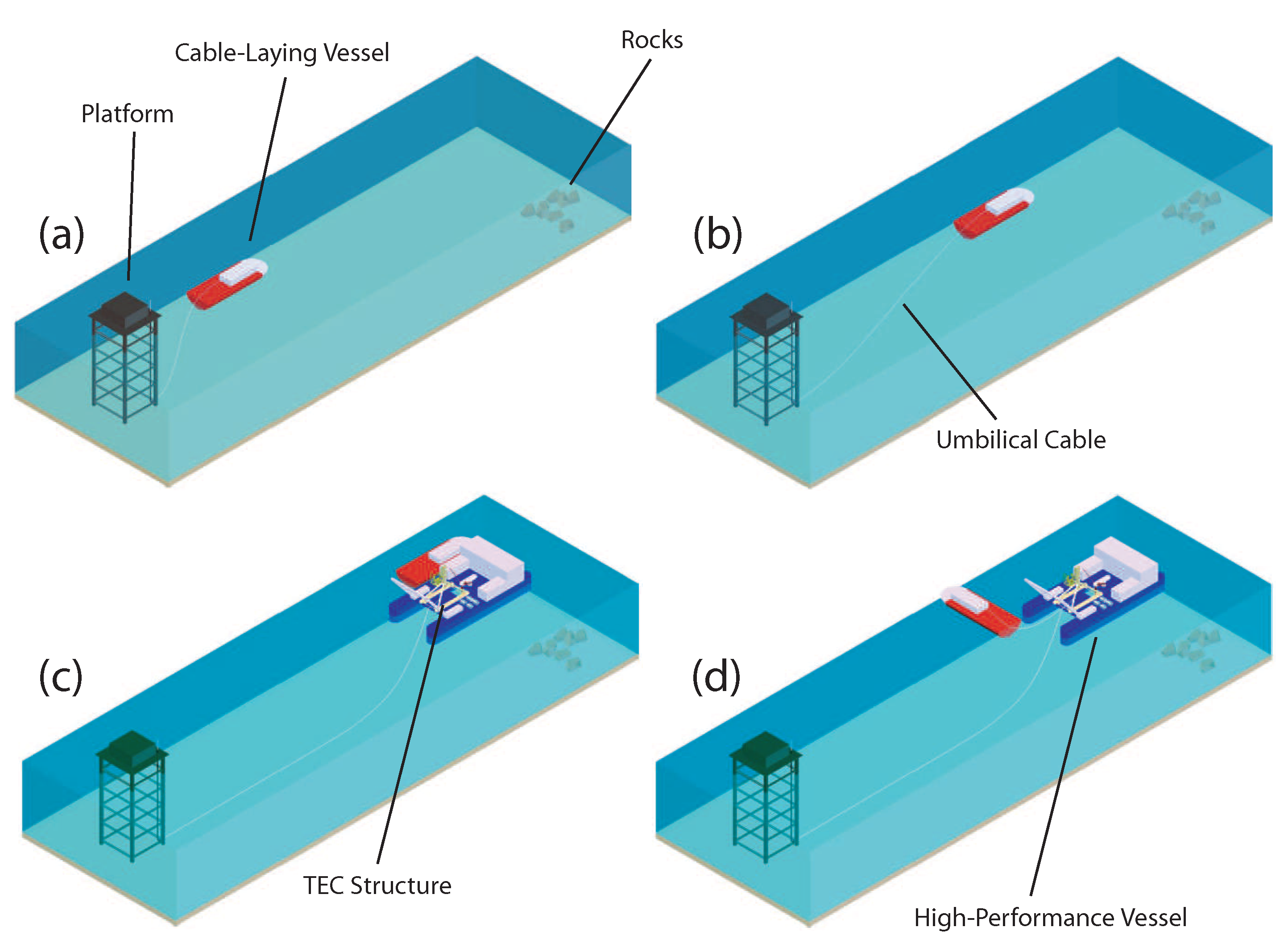
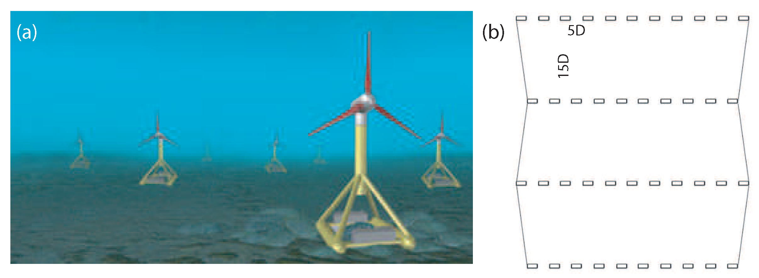
• Installation sequence at the tidal farm level: The first elements to be installed are the transformation platform and the converters. Bearing in mind the depth and the composition of the seabed on which the TEF is installed (around 40 m), the use of a jacket platform is recommended owing to the fact that it is very safe, in addition to being highly adaptable and reliable [36,37]. The following element to be installed is the exportation cable, which requires the use of a cable-laying vessel (Figure 1a). The cable-laying vessel transports the umbilical cable from the transformation platform to the special vessel in charge of transporting the TEC (Figure 1b), and the connection between the base structure and the transformation platform is, therefore, achieved (Figure 1c). The cable-laying vessel waits until the base TEC has been installed (Figure 1d), after which it is possible to install the base structure on the seabed by means of gravity (the procedure employed to install the base structure will be described below and is illustrated in Figure 2). Once the base support has been installed, the cable is extended in order to connect it to the adjacent TEC. During this procedure, the installation vessel has sufficient time to return to the base port and then return to the TEF with a new device. The cable-laying vessel waits to be given the end of the cable in order to perform the connection between the end of that cable and the new TEC structure and to repeat the cable connection process that will join it to the next TEC. This process is repeated until the TEF is completely installed.
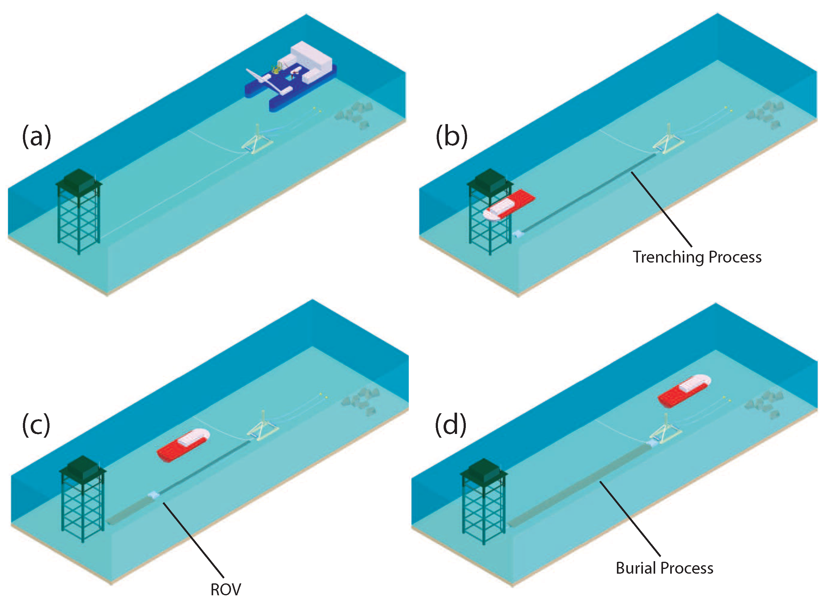
• Installation of the submarine cables: It should be noted that it is fundamental to provide the interconnection cables and the exportation cables with adequate protection in order to avoid possible natural damage (resulting from earthquakes or movements caused by waves and currents) or damage caused by human activities (anchors or fishing artifacts, among others). The protection usually employed is that of burying the cables to a sufficient depth (from 0.5 m to 1 m) [38]. The following equipment is required to install the submarine cables: (i) a cable-laying vessel with its auxiliary equipment; (ii) ROVs to perform the trenching and burial processes; (iii) tug vessels with cranes and a diving team; and (iv) ground equipment, such as excavators, winches, trucks, etc. The procedure employed is the following: the cable-laying vessel is in charge of depositing the cables on the seabed following the most homogeneous path in order to avoid zones with rocks (Figure 2a). The trenching process is carried out in the opposite direction to the cable-laying process and is performed by a ROV-trencher (Figure 2b). This device is in charge of removing the cable, making the trench and placing the cable inside the trench [39]. The same ROV (but using a different tool) then performs the burying process in the opposite manner to the trenching process, thus leaving the cable completely covered (Figure 2c,d).

2.1. Manual Installation and Maintenance Maneuvers for First Generation TECs

We define the term manual for installation and maintenance maneuvers for TECs in an open loop. These sorts of maneuvers are currently used in the first generation tidal technologies which are, at present, in a pre-commercial stage [38]. An example of the gravity-based TEC described in this section and designed by the GIT-ERM research group is illustrated in Figure 3. The manual installation of the TECs can be divided into the installation sequence for the support structure of the TECs and the installation sequence for the gondolas. The following steps have, therefore, been defined in order to perform the installation tasks:

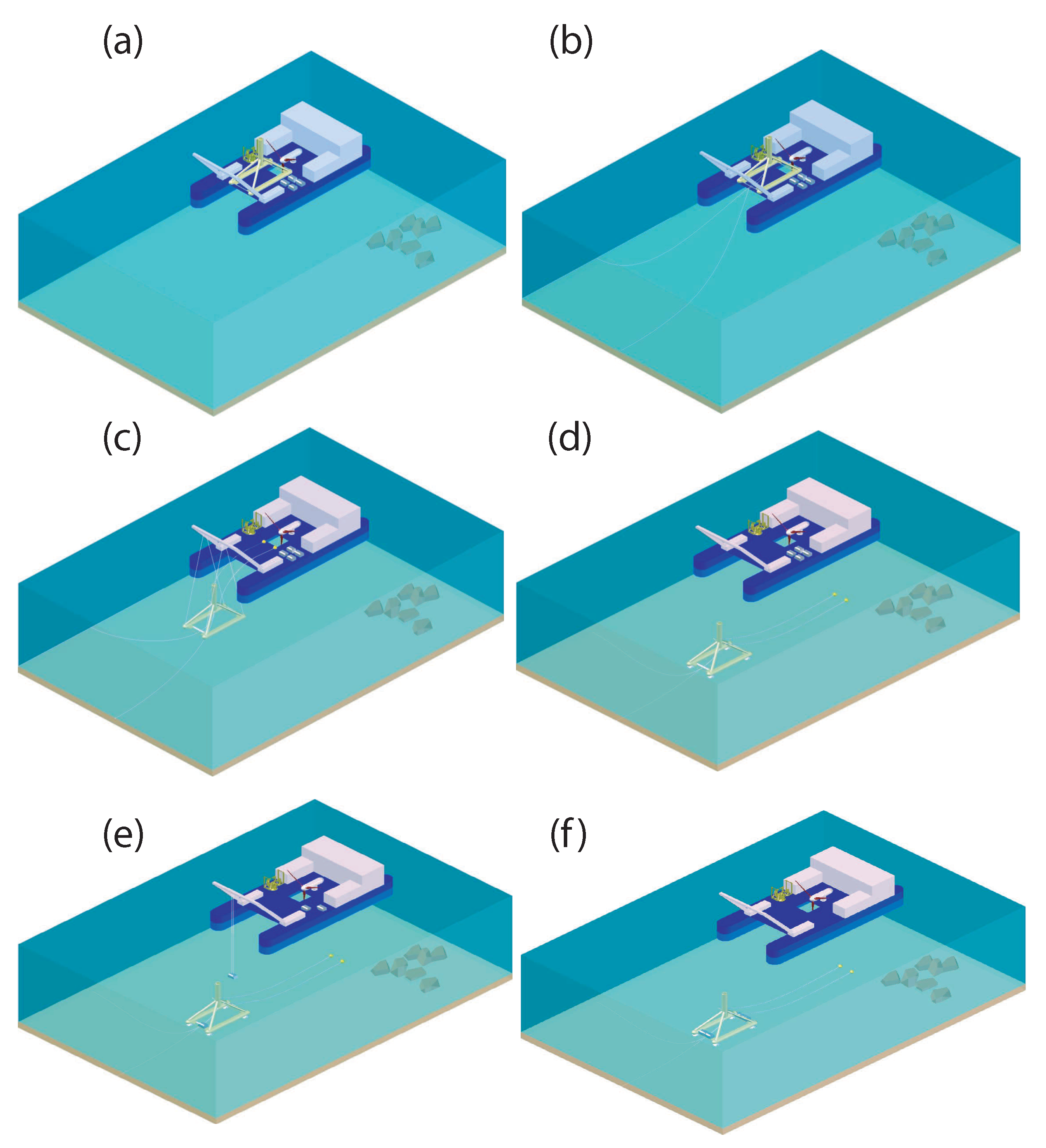
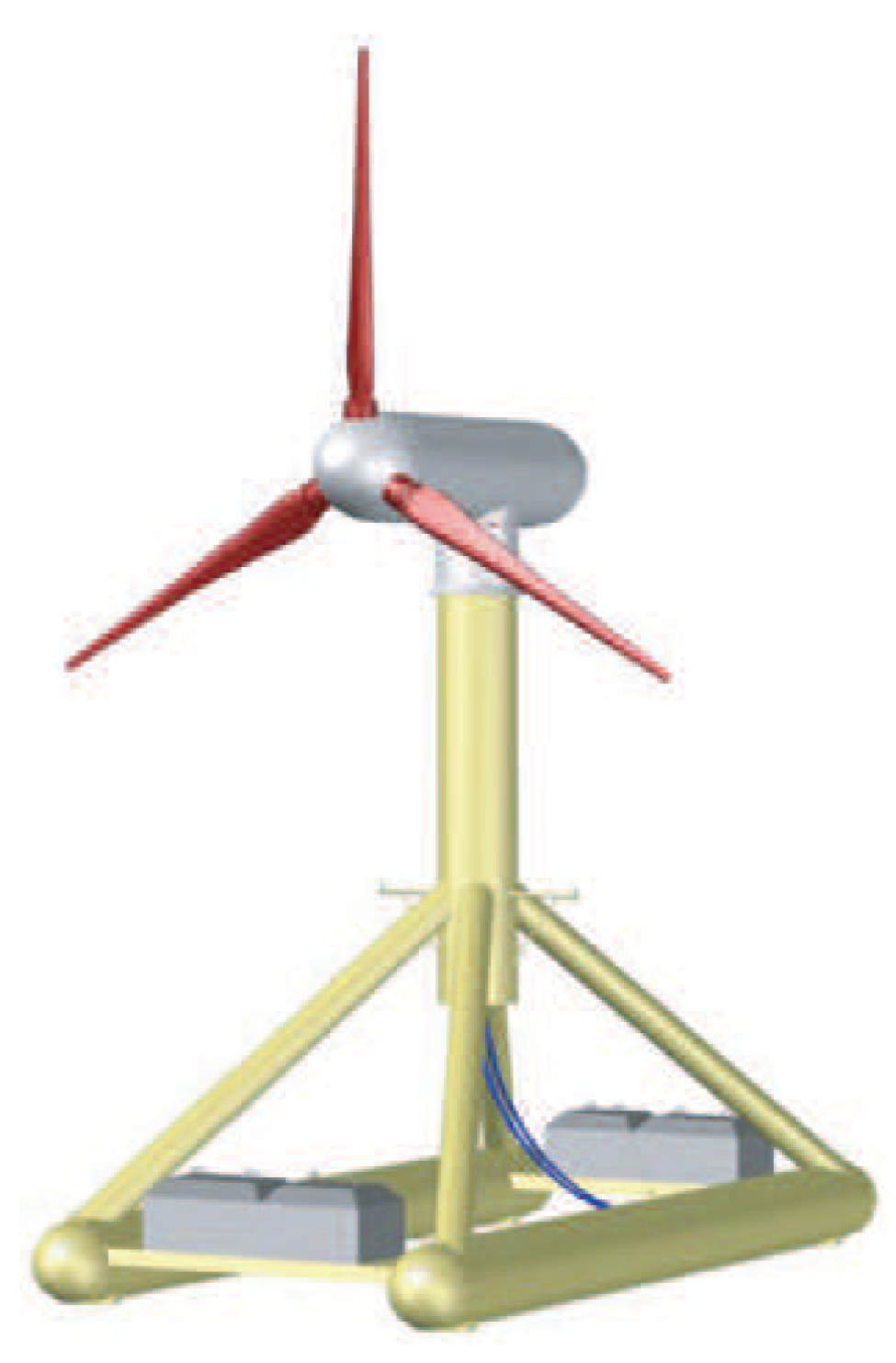
• Installation of the support structure of the TECs:

  -

  The special vessel transports the complete TEC and the equipment required (support structure, ballasts, gondola, etc.) simultaneously (see Figure 4a), and moves from the base port towards the TEF. When it is at the TEF, it uses its dynamic positioning system to place all the necessary items in the exact position in which the TEC will be installed.

  -

  The umbilical cables are then connected to the base structure and the guide cables used to recover the gondola are attached to the deck of the vessel, thus preparing the TEC structure for its installation (see Figure 4b).

  -

  The crane on the special vessel raises the TEC structure off the special vessel by means of four cables, and the descent process begins. The descent process is performed thanks to the weight of the TEC structure and the guide cables, and the descent velocity and the orientation of the TEC structure with regard to the special vessel are controlled (see Figure 4c). When the structure is correctly positioned, special concrete bags are released in order to fix the TEC structure to the seabed (see Figure 4d). The cables used during the descent process are subsequently removed.

  -

  The ballasts are placed on the TEC structure. This operation is performed by the crane, and the ballasts are lowered one by one (see Figure 4e).

  -

  Finally, the guide cables are detached from the vessel and are submerged by means of a ballast and a buoy in order to recover them during the future gondola installation process. These cables are placed on the seabed in a zone that does not involve risks as regards the installation procedures of the other devices, the farm or the umbilical cables. The TEC structure is now considered to be completely installed (see Figure 4f).

• Installation of the gondolas:

  -

  Once the support structure has been completely installed, the special vessel is placed on the TEC structure and the guide cables of the gondola are recovered by means of an acoustic signal (see Figure 5a).

  -

  In order to work with the gondolas, a specific tool equipped with a hydraulic system will be used, whose objective is to wrap itself around the gondola that is to be installed or recovered. Its operation is similar to that of a clamp (see Figure 6).

  -

  The guide cables are connected to the tool used to lower the gondola (see Figure 5b). These cables facilitate the descent of the gondola and the insertion of the gondola into the structure.

  -

  The gondola initiates its descent with the guide cables thanks to its own weight and without oscillations until the gondola has been inserted into the structure. Figure 5c illustrates the descent process of the gondola and Figure 5d depicts the gondola-structure insertion process.

  -

  The final step is that of removing the tool used to install the gondola and the retrieval of the guide cables. Figure 5e illustrates the removal process. When the tool is on the deck of the vessel, the guide cables are removed from the tool and are submerged in a safe location by means of a ballast and a buoy in order to recover them during the next intervention. Figure 5f shows the installation of the whole TEC once the process has been completed.

The maneuvers that are necessary to perform the maintenance tasks (recovery of a submerged gondola) follow the inverse order of that described for the installation of the gondola. The procedure for maintenance maneuvers, therefore, shares a lot of similarities with the procedure of installing the gondolas, and the steps required to perform maintenance maneuvers are the following:

• Recovery of a submerged gondola:

  -

  The starting point is that of locating the special vessel above the gondola to be recovered. The first step is the recovery of the cables from the seabed. The ends of the cables are released from the seabed by means of an acoustic signal (see Figure 7a) and these cables are connected to the tool used to recover the gondola.

  -

  The tool starts its descent, following a trajectory with an inclination angle that permits the tool to wrap itself around the back of the gondola (see Figure 7b).

  -

  When the tool is ready to perform the grip, the cables are tightened and placed completely vertically (see Figure 7c). The hydraulic system of the tool is activated in order to close it and fix it to the gondola (see Figure 7d).

  -

  The process of raising the gondola begins. As the cables are tightened, the displacements are very small and the operation is carried out under safe conditions (see Figure 7e).

  -

  When the whole system (gondola + tool) is outside the water, the cables are removed from the tool and are submerged again by means of a ballast and a buoy in order to recover them in the future (see Figure 7f).

2.2. Automated Installation and Maintenance Maneuvers for First Generation TECs

Section 2.1 shows that the manual installation and the maintenance maneuvers are both very complex and very costly. Moreover, the zones in which tidal energy technologies operate economically are zones with peak tidal velocities greater than 2.5 m/s [40,41] and are also characterized by the fact that they are zones with adverse climatologic conditions that increase the complexity of these maneuvers [42]. The development of automated installation and maintenance maneuvers, which help to reduce the resources required, the complexity of the operations and the costs are, therefore, a very interesting point to research. We define the term automated for TEC installation and maintenance maneuvers in a closed loop. These sorts of maneuvers have recently been presented by the GIT-ERM research group through several recent patents [43,44,45] as a solution that will influence tidal energy systems in the following particular aspects [22,23]: (a) the number and duration of the installation operations will be reduced; (b) the profitability of the project will be increased; (c) there will be less human intervention; (d) the weather window will be maximized, and (e) it may be possible to employ general-purpose ships as tugboats for maintenance purposes, rather than high-cost specialist vessels. In the following subsections, we provide details on the modifications developed by the GIT-ERM research group and made to the TEC proposed in Figure 3 in order to perform automated immersion and emersion maneuvers, along with the definition of the procedures employed to install and maintain these advanced systems.

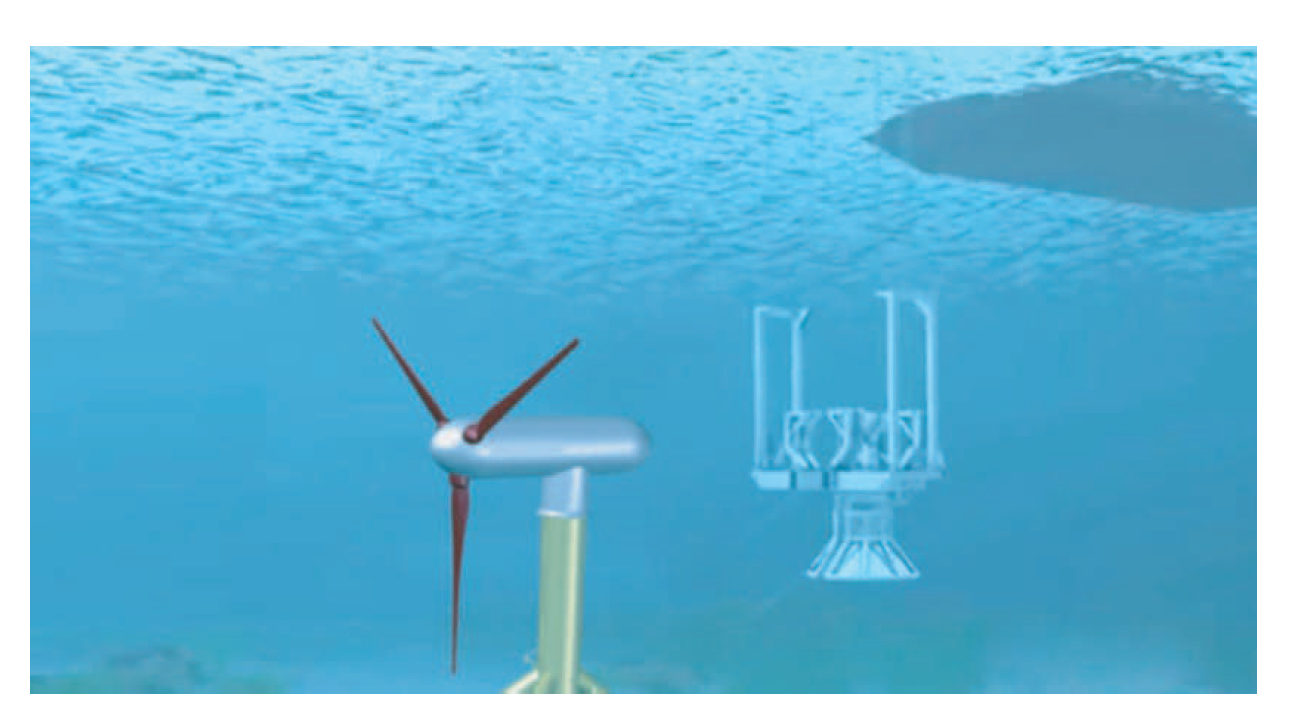
2.2.1. Modifications Made to TECs in Order to Perform Automated Maneuvers

The GIT-ERM research group designed the gravity-based first generation TEC presented herein in order to enable it to perform automatic emersion/immersion maneuvers. This is done by using small guide wires and controlling the ballast water inside the device [24,25]. The control of the ballast water permits the implementation of a closed-loop depth and/or orientation control, which, in turn, allow(s): (i) the extraction of the main power generation unit from its normal depth of operation (on the seabed) to the surface of the sea, and (ii) it to be returned from the surface to its base on the seabed. Figure 8 illustrates the shape of a gravity-based first generation TEC capable of performing automated maneuvers and its distribution equipment. The main differences between the gondola of the TEC illustrated in Figure 3 (designed for manual maneuvers) and the gondola of the TEC depicted in Figure 8 (designed for automated maneuvers) are the following: (a) the places in which the ballast tanks and their associated pumping system are located, and (b) the shape of the gondola, which has been modified in order to attain neutral buoyancy when the ballast tanks are half full. In the system depicted in Figure 8a, the gondola has been increased longitudinally as opposed to increasing its diameter. This has been done so as to optimize its hydrodynamic performance [37]. A detailed description of the design modifications and the behavior of the modified gravity-based TEC, along with interesting laboratory experiments, can be found in [23,24,25,37].

2.2.2. Automated Installation and Maintenance Maneuvers

In this section, we propose a procedure with which to carry out the automated installation and maintenance maneuvers for gravity-based first generation TECs by controlling the inner ballast water inside the device in order to place the TEC at the desired depth. In the procedure proposed, it will be noted that the degree of complexity of the maneuvers is substantially reduced, as are the means required, which will translate into a substantial reduction in costs. As in the previous section, the installation of the TECs can be divided into the installation sequence of the structure of the TECs and the installation sequence of the gondolas. The following steps have, therefore, been defined in order to perform the automated installation tasks:

• Installation of the base structure of the TECs: Note that the structure of the TECs designed for manual maneuvers is the same as the structure designed for automated maneuvers. The installation methodology of the structure of these TECs is, therefore, similar to that used in traditional installation maneuvers.
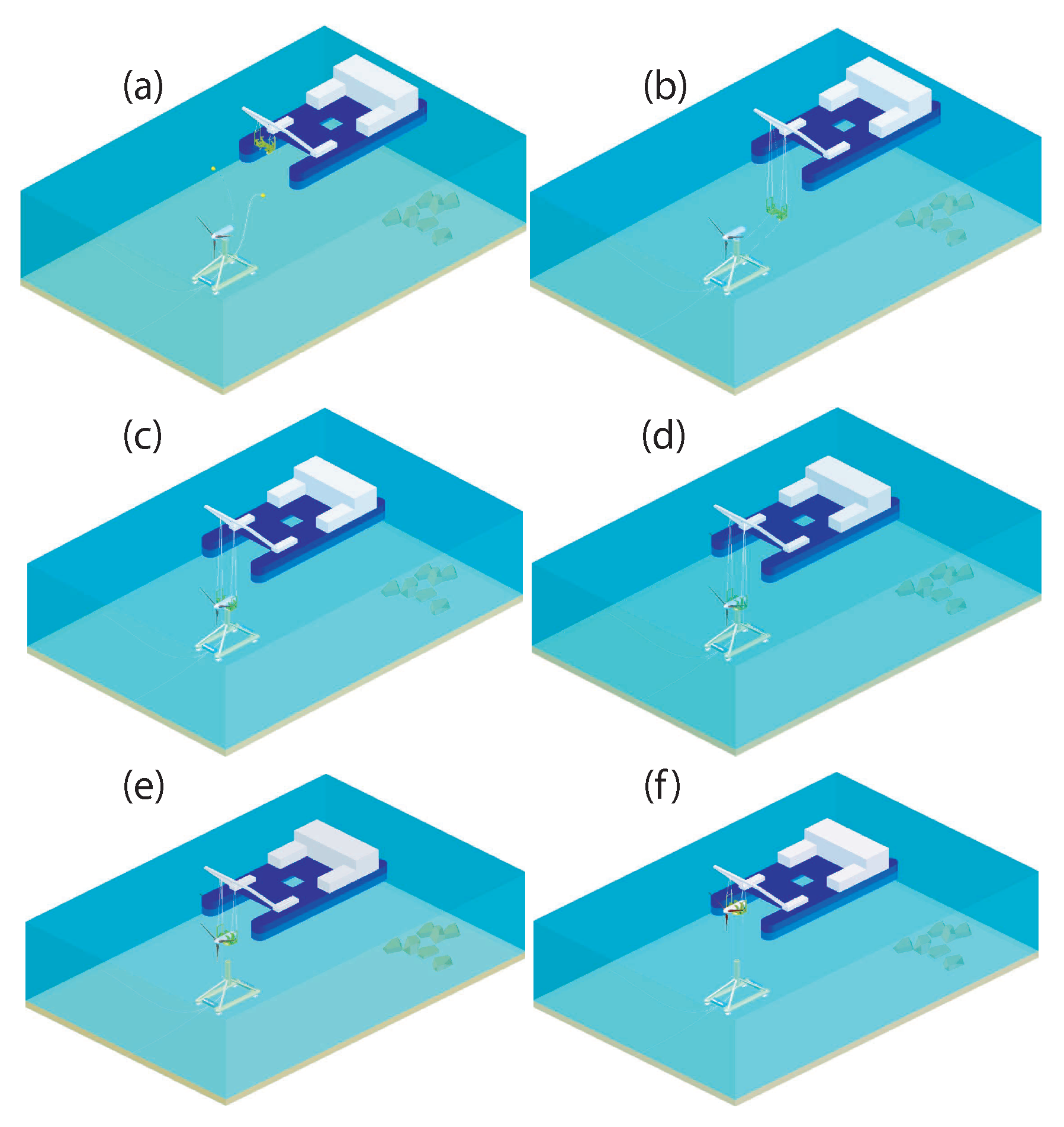
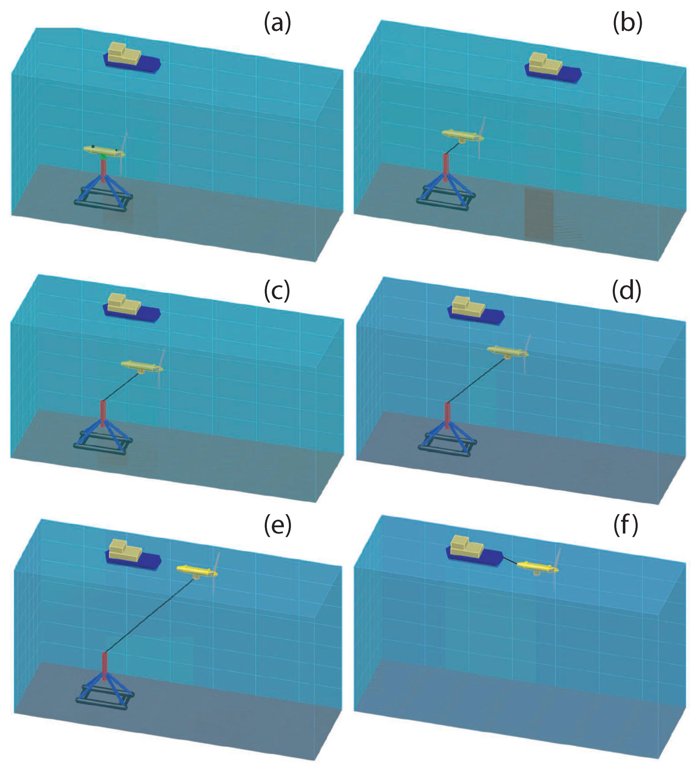
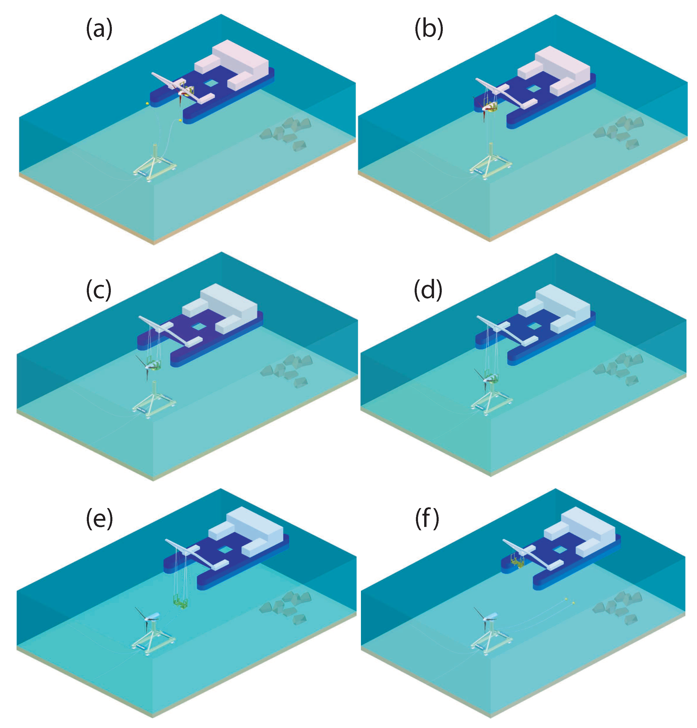
• Installation of the gondolas (immersion sequence): As the gondola is modified to be able to perform automated maneuvers, the installation sequence of the gondolas is different to that used in traditional maneuvers. Figure 9 provides a graphical sequence of the complete process, which is detailed as follows:

  -

  Once the base structure that supports the gondola is completely installed, the gondola is moved using a tugboat. The tugboat will move one gondola per trip (see Figure 9a).

  -

  When the tugboat arrives in the position in which the gondola will be placed, the guide cables connected to the structure of the TEC are recovered by using an acoustic signal (see Figure 9b).

  -

  In the following step, the gondola is lowered onto the seabed. The inner ballast water inside the device is controlled, signifying that the gondola starts filling with water and its inner ballasts permit the gondola to descend. If the difference between the weight of the gondola and the buoyancy force is small, the descent process will be performed slowly. The descent velocity is completely controlled by changing the amount of water inside the inner ballasts (see Figure 9c,d). The gondola descends to a depth close to the base structure that will support the gondola.

  -

  When the gondola is at the desired depth, but not in a vertical position as regards the base structure owing to the tidal currents, the guide cable will help install the gondola on the base (see Figure 9e).

  -

  When the gondola is on the structure of the TEC, the inner ballasts of the gondola are filled with water in order to achieve an adequate coupling with the base structure. The installation of the TEC is, therefore, completed (see Figure 9f).

The maneuvers that are necessary to perform the maintenance tasks (recovery of a submerged gondola) in a closed loop follow an inverse order to that described for the installation of the gondola. The steps required to perform maintenance maneuvers are the following:

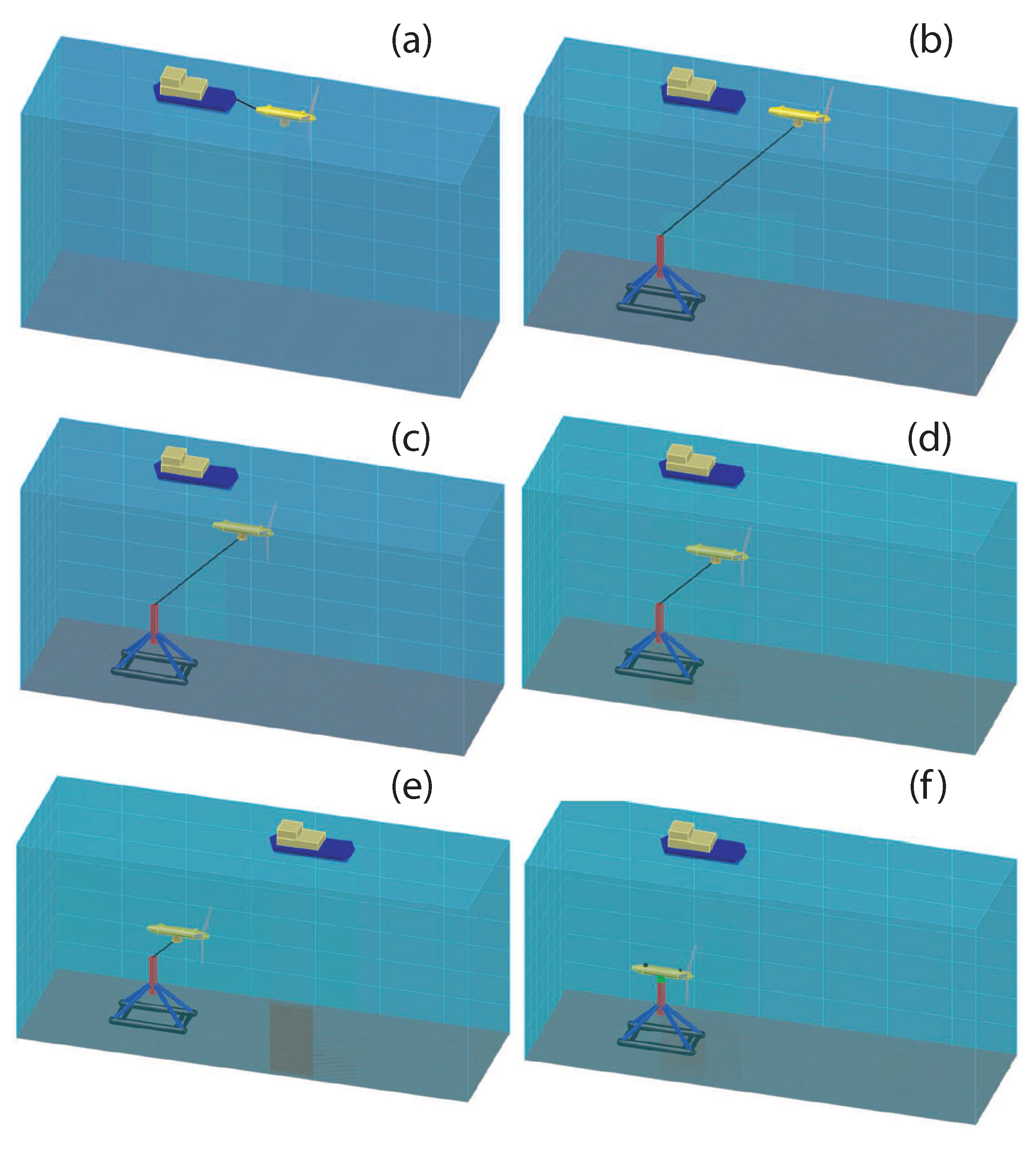
• Recovery of a submerged gondola (emersion sequence):Figure 10 shows a visual sequence of the procedure, and a detailed description is provided below.

  -

  When the gondola is on the structure of the TEC (see Figure 10a), water begins to empty out of the inner ballasts of the gondola until the structure of the TEC and the gondola separate (see Figure 10b).

  -

  The controlled emersion process of the gondola now begins. Water is emptied out of the inner ballast of the gondola in a controlled manner in order to obtain a smooth emersion movement (see Figure 10c,d). A guide cable is used during the emersion process.

  -

  When the gondola is on the surface of the sea, the inner ballast is completely emptied in order to increase the buoyancy of the gondola, after which, the control system is disconnected.

  -

  The maintenance tasks are carried out on the gondola (see Figure 10e). When these tasks have been completed, the control system is connected and the gondola starts filling its inner ballasts with water, thus allowing the gondola to descend automatically (see Figure 10f).

  -

  All the steps explained for the installation of the gondola (immersion maneuver) are repeated to achieve the connection between the base structure of the TEC and the gondola.

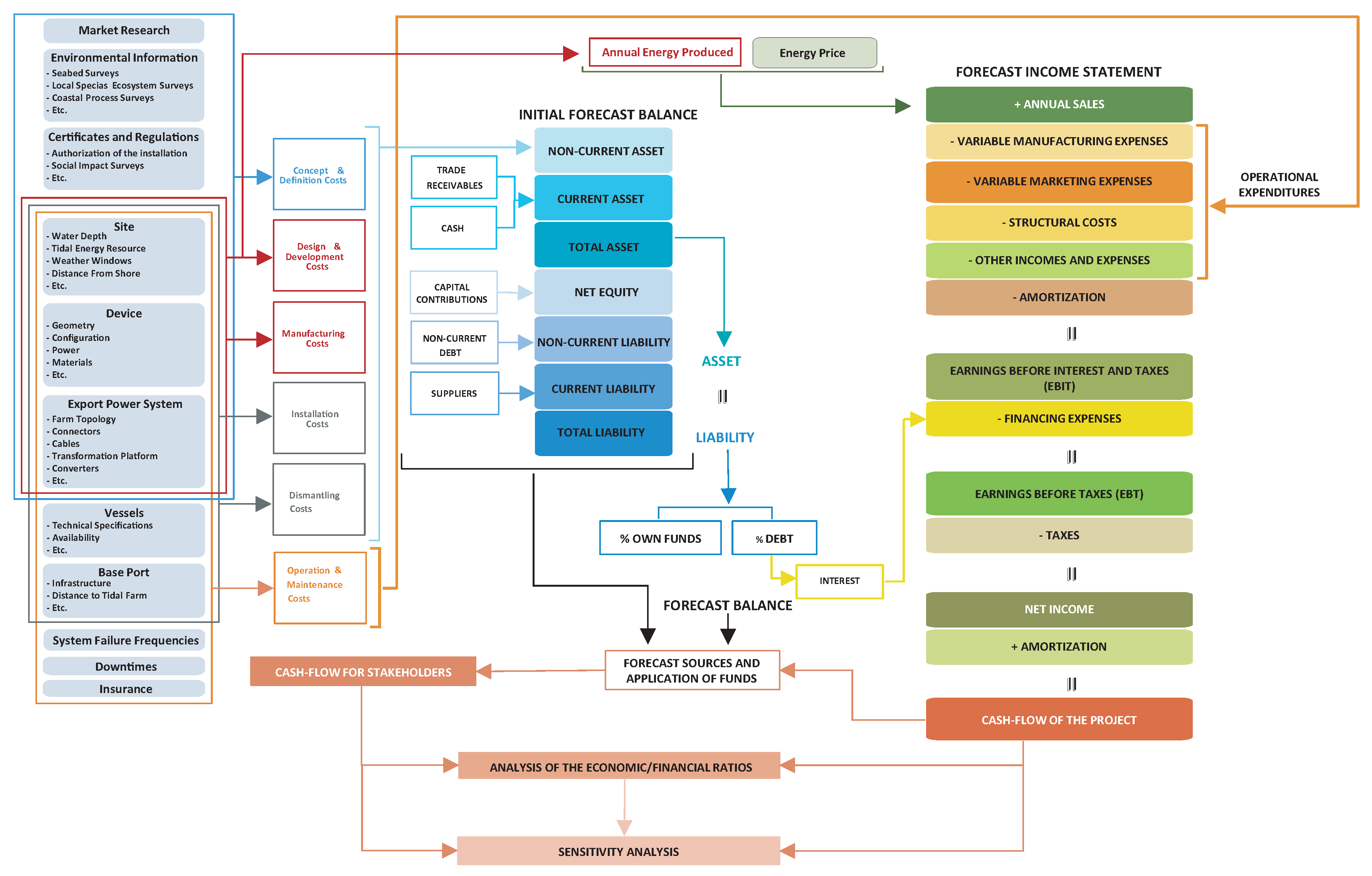
3. Economic-Financial Feasibility Procedure

The objective of this procedure is to forecast the eventual profitability of the investment as regards both the project itself and the stakeholders. This will allow those involved to decide whether or not the project is financially viable. The proposed model, which is shown in Figure 11, has the following stages [19,46]: (i) the LCC of the project is studied and the annual sales estimated; (ii) the financing structure of the model is determined; (iii) the forecast income statement, forecast balance and forecast sources and application of funds for the lifespan of the project are defined; (iv) the cost–benefit analysis is obtained, which is done by utilizing the forecast cash-flows of the project, along with the forecast sources and application funds; (v) the most important financial rations of the model are studied, and (vi) a sensitivity analysis is carried out in order to detect possible business risks. The following subsections deal briefly with this.

3.1. Study of the Costs throughout the Service Life of the Project and Estimation of the Annual Sales

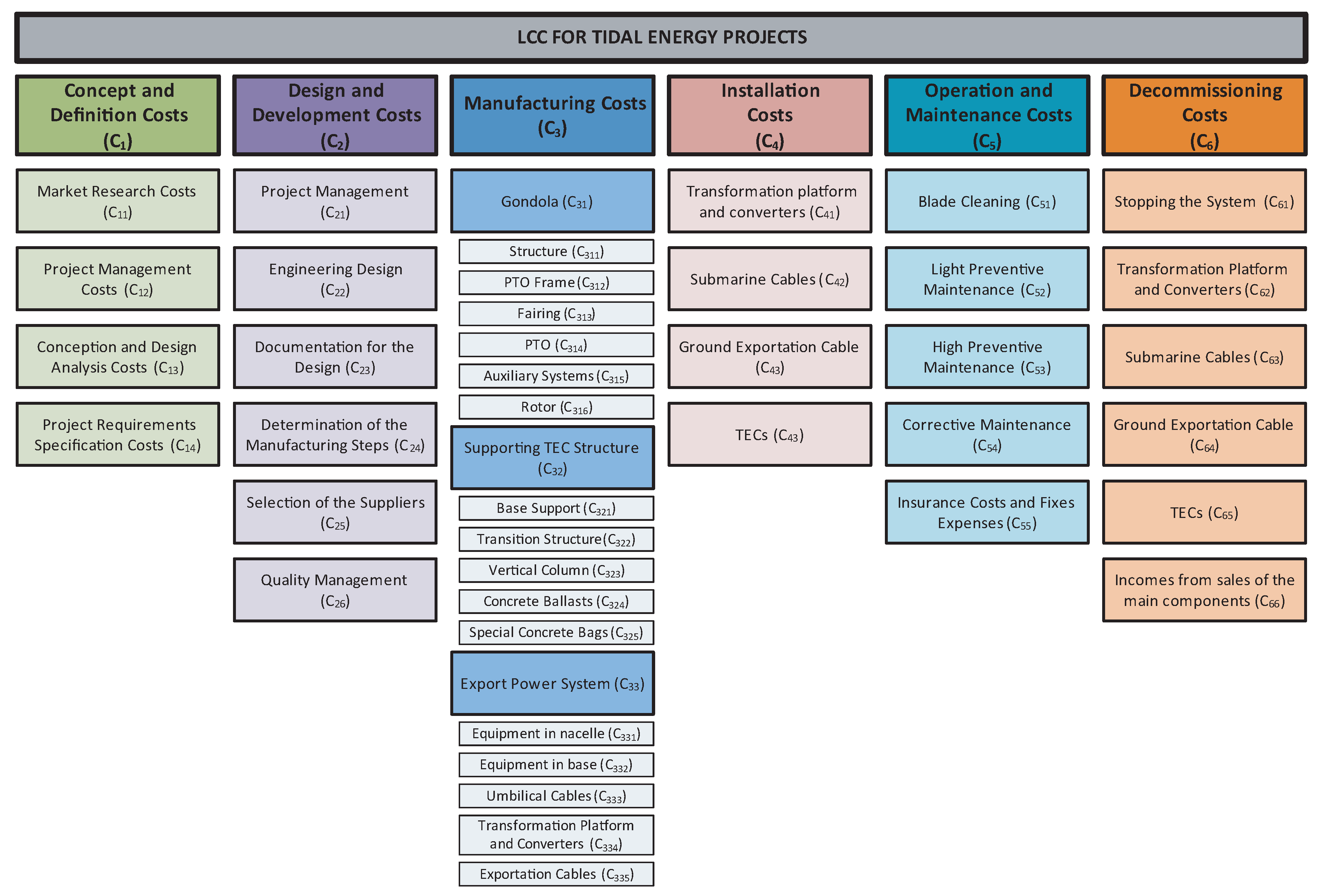
The study of the fundamental variables of the economic model implies the definition of the LCC of the project [26,47] and the estimation of the annual sales. Please note that we obtained the estimated costs and estimated annual sales included in the economic feasibility procedure for tidal energy projects (TEPs) by carrying out an analysis of current scientific literature and reports created by companies that specialize in these types of technologies and shipyards.

3.1.1. LCC for TEPs

The LCC is, in essence, an accounting structure containing the mathematical formulations that can be used to estimate the associated costs of the projects during their lifespan [48]. The benefits obtained as a result of determining the LCC of these sorts of projects are summarized as follows [49,50]: (i) the life cycle concept results in earlier actions by which to generate revenue or in lower costs than might otherwise be considered; (ii) better decisions can be made as the result of a more accurate and realistic assessment of revenues and costs, at least within a particular life-cycle stage; (iii) it can promote long-term rewarding in contrast to short-term profitability rewarding; (iv) it provides a better understanding as regards the difference between the acquisition costs and the operating and support costs, and (v) it encourages businesses to find a correct balance between investment costs and operating expenses. In the particular case of TEPs composed of first generation TECs, the stages of which the LCC of the proposed methodology is composed are the following (see also Figure 12). A detailed description of all the structures of the subcosts and the subsequent procedure employed to compute them can be found in [19,46]:

• Concept and definition costs ($C_1$): These costs correspond to those activities whose objective is to guarantee the feasibility of the project. The costs typically included are the following: (i) market research costs; (ii) project management costs; (iii) conception of the tidal farm and design analysis costs; and (iv) project requirement specification costs.
• Design and development costs ($C_2$): These costs comprise the specification of the requirements of the project and also provide proof that the project has been carried out. They typically include costs regarding: (i) the management of the project; (ii) a technical design and activities for the protection of the environment; (iii) the documentation required for the design; (iv) the definition of the manufacturing steps for the TEF; (v) the inclusion of the selected suppliers; or (vi) quality management.
• Manufacturing costs ($C_3$): These encompass all the costs of manufacturing the elements employed to construct the tidal energy farm and, at this stage, principally consist of: (i) the gondola; (ii) the support structure of the TEC; and (iii) the export power system.
• Installation costs ($C_4$): These are related to the activities required to install all the elements required to construct the TEF, which are, at this stage, typically: (i) the installation of the transformation platform and converters; (ii) the installation of the submarine cables; (iii) the installation of the ground exportation cable; and (iv) the installation of the TECs.
• Operation and maintenance costs ($C_5$): These are all the costs of exploiting the tidal energy project, and include: (i) blade cleaning; (ii) light preventive maintenance; (iii) high preventive maintenance; (iv) corrective maintenance; and (v) insurance costs and fixed expenses.
• Decommissioning costs ($C_6$): These concern the activities required to remove and dispose of the components related to the project, so as to leave the sea as it was before the project started. The principal costs are, in this case: (i) stopping the system; (ii) dismantling the transformation platform and the converters; (iii) dismantling the submarine cables; (iv) dismantling the exportation cable; (v) dismantling the TECs; and (vi) incomes obtained from the sales of the main components (this value will be modeled in the cost structure as a negative value because it is an income).

Once these costs have been computed, the total LCC of a TEP yields the following result:

$$LC{C}_{TEP}=C_1+C_2+C_3+C_4+C_5+C_6.$$

(1)

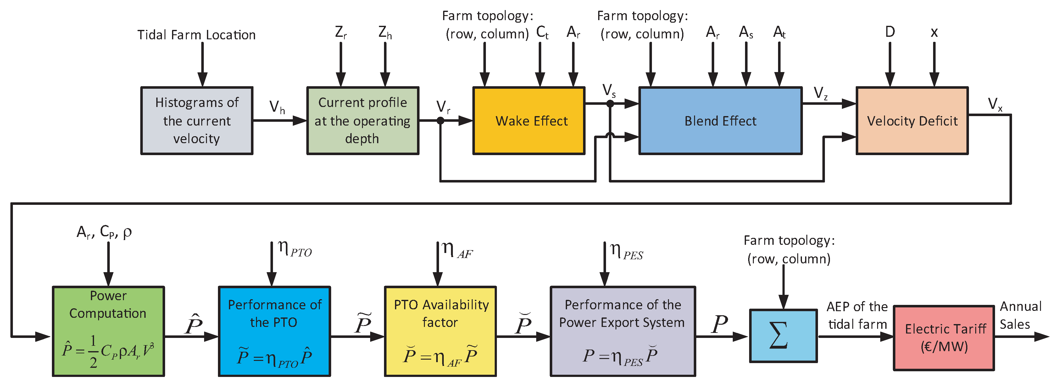
3.1.2. Estimation of the Annual Sales

If the electric tariff is known, then it is possible to estimate the annual sales (AS) attained from a TEP, which are directly related to knowing the annual energy produced (AEP) by the TEF. One of the most important indicators employed to discover whether it will be possible to commercially exploit a particular project is the estimation of the AEP, which usually depends on: (i) the information concerning the site; (ii) the devices used in the TEF; (iii) the energy export system; (iv) the characteristics of the current; (v) the ability of the device to capture energy; and (vi) the ability to convert and export the energy. The procedure employed to accurately estimate the AEP is shown in Figure 13, while the following expressions are required to compute the AEP for a TEF. A detailed description of the procedure developed (based on actuator disk theory) can be found in [46]:

$$\begin{array}{c}{V}_r=V_h·{\left(\frac{Z_r}{Z_h}\right)}^{\frac{1}{7}},\hfill \\ a=1-\sqrt{1-c_t};A_s=\left(\frac{1-0.5a}{1-a}\right)·A_r;V_s=(1-a)·V_r,\hfill \\ A_s·V_s^2+\left(A_t-A_r\right)·V_r^2=A_t·V_z^2,\hfill \\ V_x=\left(V_s-V_z\right)·e^{-0.2\frac{x}{D}},\hfill \\ AEP=\sum _{i=1}^{N_{row}}\sum _{j=1}^{N_{column}}P(i,j),\mathrm{where}P(i,j)=\frac{1}{2}·C_P·\rho ·A_r·V_x^3(i,j)·{\eta }_{PTO}·{\eta }_{AF}·{\eta }_{PES},\hfill \\ AS=p_{ET}·AEP,\hfill \end{array}$$

(2)

where $V_r$ symbolizes the velocity of the rotor, $V_h$ expresses the velocity on the sea surface, $Z_r$ denotes the depth of the rotor, $Z_h$ represents the water column depth, a symbolizes the axial induction factor, $c_t$ denotes the thrust coefficient, $V_r$ represents the free stream velocity at the rotor depth, $A_r$ is the surface of the rotor, $V_s$ denotes the flow velocity at the rotor of the turbine, $A_s$ represents the output flow surface, $A_t$ symbolizes the total frontal surface of the TEC, $V_z$ expresses the final velocity of the blended flow, D denotes the diameter of the rotor, (x, $V_x$) represents an intermediate point located between the rotor output and the blend flow downstream, $N_{row}$ and $N_{column}$ are, respectively, the number of rows and columns on the farm, $C_P$ denotes the power coefficient, $P(i,j)$ denotes the power of the TEC located in row i and column j on the farm, $\rho$ symbolizes the fluid density, ${\eta }_{PTO}$ is the performance of the power take off (PTO), ${\eta }_{AF}$ denotes the availability factor, ${\eta }_{PES}$ represents the performance of the power export system and, finally, $p_{ET}$ is the electric tariff.

3.2. Financing Structure of the Model

The following step involves defining the financial structure employed to define the resources required in the financial model. It is possible to consider the funding sources shown as follows [51]: (i) own funds, which will initially consist of the capital invested by stakeholders and, as time progresses, the resources of the project itself, which will consist of the initial stakeholders’ contribution and the reserves (project profits which are achieved and not distributed); and (ii) external resources from financial institutions that must be returned by the organization.

3.3. Forecast Balance, Forecast Income Statement, and Forecast Sources and Application of Funds in the Model

The way in which the forecast balance, the forecast income statement and the forecast sources and application of funds are obtained is fundamental to understand what will occur, or may occur, in the future of the project [52]. These concepts will be briefly developed below, and a detailed description of these instruments can be found in [46].

3.3.1. Forecast Balance

The tool that allows the clarification of what is occurring in the project on the basis of the available accounting information is the forecast balance, which takes into account the situation of the project’s assets, consisting of the project’s debts, capital, rights and assets at a particular time. The asset of the forecast balance comprises the rights and the assets, while information regarding the financing attained is obtained from the net equity and the liability. The patrimonial masses of the forecast balance are the following: (i) the current asset, which includes those assets that are not initially permanent in the project owing to the fact that their remain period is under a year, and the non-current asset, which refers to all those assets that will remain in the project for over a year. The sum of these patrimonial masses, meanwhile, allows us to determine the total asset and, therefore, the total liability, whose components are the following: (i) the net equity, which comprises all the items that are not contemplated as obligations; (ii) the non-current liability, which considers all debts that remain in the project for more than a year, and (iii) the current liability, which comprises all debts whose remain period is under a year.

3.3.2. Forecast Income Statement

The forecast income statement is employed to quantify an exercise’s profit or loss and to discover how it was created. This is done by carrying out an analysis of each item of expenditure with regard to incomes. It is possible to classify the expenses and incomes of this type of projects in the following manner: (i) the annual sales (AS), i.e., the incomes attained after operating the project; (ii) the operational expenditures (OPEX), including operation and maintenance costs, administrative costs, taxes, rent, insurance, etc.; (iii) the amortization (AM) during the period as regards plant and equipment, the attrition of property and intangible assets; (iv) the financing expenses (FE), including the project’s incomes and financial expenses, and (v) the corporate taxes (T), in which the taxes on the benefits of the period that are different from the other taxes paid by the corporation (and which are normally viewed as structural expenses) are considered. All these expenses are used to organize the forecast income statement in the following manner:

$$\begin{array}{c}EBIT=AS-OPEX-AM,\hfill \\ EBT=EBIT-FE,\hfill \\ NI=EBT-T,\hfill \end{array}$$

(3)

where EBT represents earnings before taxes, NI denotes the net income, EBIT symbolizes earnings before interest and taxes and $C{F}_p=NI+AM$ is the cash-flows of the project.

3.3.3. Forecast Sources and Application of Funds

The forecast sources and application of funds allow us to to attain the variations that took place in the project’s patrimonial masses. This is done by contrasting them in two accounting periods with the aim of discovering the sources obtained in that period of time as a consequence of the exploitation cycle of the project, and where they were employed. This makes it possible to discover the project activity’s efficiency and comprises: (i) the project resources admitted that year, and how they were applied, and (ii) what effect this movement of inflow and application had on the current asset. The forecast sources and application of funds make it possible to determine the stakeholders’ cash-flow, i.e., the cash-flow that it would be possible to disperse in dividends in the case of there being no debt [53].

3.4. Analysis of the Economic and Financial Ratios

By analyzing the economic-financial ratios, it is possible to analyze the project’s solvency, liquidity and profitability in order to ascertain its feasibility. We shall, therefore, analyze the ratios shown below so as to determine what strengths and weaknesses these types of projects have [52]:

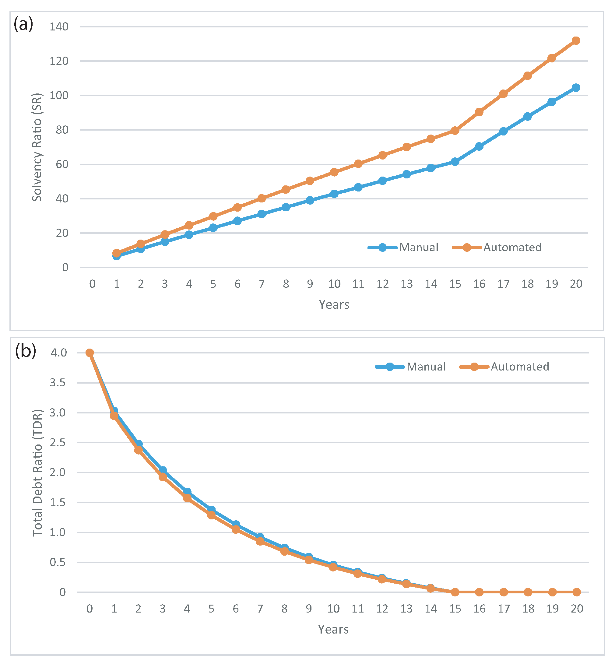
• Financial Ratios: The information obtained in the forecast balance is utilized to determine the project’s short-term situation and its liquidity, in addition to its degree of long-term sustainability and its solvency. The following financial ratios will be studied: (i) Solvency Ratio (SR), which will make it possible to ascertain how effective the project must be if it is to produce sufficient liquid financial resources in order to punctually meet its commitments as regards the payment of short-term debts resulting from their cycle of operation, in addition to the short-term practicable payments in the same cycle, and (ii) Total-Debt Ratio (TDR), which makes it possible to determine the financial dependence degree by means of the structural composition of funding sources.
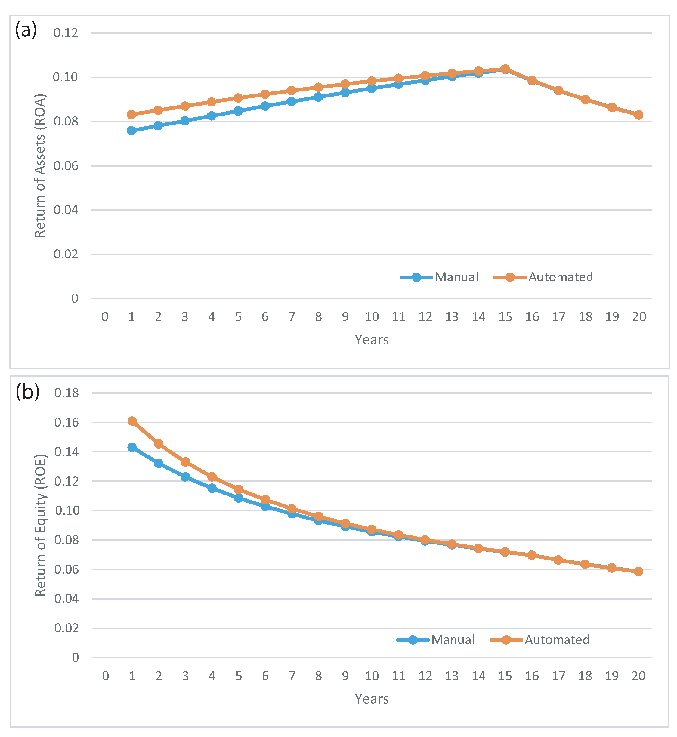
• Economic Ratios: These make it possible to discover whether the assets are efficiently employed with regard to the management of the operations of said project. The following ratios are employed: (i) Return of assets (ROA), which shows how effective the assets are as regards producing value and; (ii) Return of Equity (ROE), which illustrates how effective the capital contributed by the investors has been. This depends on the net income attained that year.

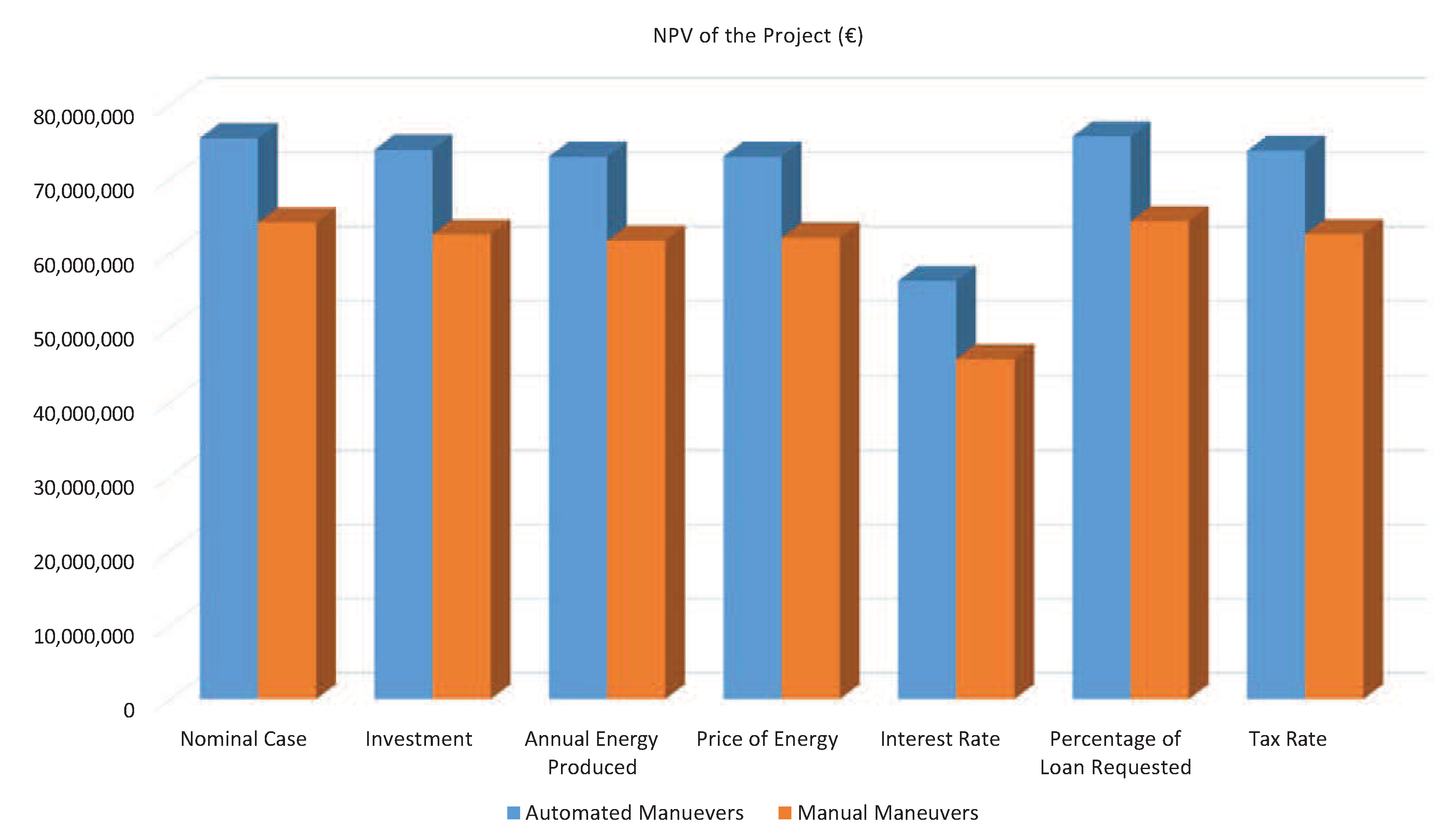
3.5. Sensitivity Analysis

In order to determine the variables that most affect the viability of the project, it is important for performing a sensitivity analysis with the objective of analyzing the behavior of the project in different situations. The analysis of these scenarios is performed by means of the computation of the net present value (NPV), the internal rate of return (IRR) and the discounted payback period (DPBP), which have an extended application in scientific literature [54]. In these sorts of renewable energy projects, the parameters that are, in principle, expected to influence the project profitability are the following: (i) Investment; (ii) AEP; (iii) Price of energy; (iv) Interest rate; (v) Percentage of loan requested, and (vi) Tax rate.

4. Case Study

The installation and maintenance maneuvers defined in Section 2, along with the economic-financial methodology shown in Section 3, will now be applied to a case study consisting of a 50 MW TEF. This farm is composed of gravity-based first generation TECs and is located in the Alderney Race, which is one of the Channel Island Races in the United Kingdom (UK). This will be done in order to determine the viability and profitability of the project from the economic-financial point of view, when using either manual or automated maneuvers, together with the realization of a sensitivity analysis. The analysis will be carried out in an attempt to show that automating these maneuvers will improve the future competitiveness of tidal systems. It may also allow us to detect business risks in the case of the oscillation of fundamental variables of the model, such as investment, the annual energy production, the price of energy, the interest rate, the percentage of loan requested or the tax rate. We shall deal with all of the aforementioned aspects below.

4.1. Description of the Design and Economic-Financial Parameters

The proposed tidal energy farm will consist of 42 1.2 MW TECs, each of which will have an open rotor configuration with their axes parallel to the flow (Figure 14a). It is possible to separate the gondola of the TEC from the structure, which facilitates maintenance tasks. However, the orientation of the gondola is fixed when it is mounted on the structure, and it is consequently mandatory to have a pitch controllable blade system with the aim to maximize the energy that is captured in both current directions. The blades have a diameter of 20 m, while the TEC is attached to the seabed by gravity. The TEF will consist of four rows, and there will be 11, 10, 11, and 10 TECs in each row (Figure 14b). This will make it possible to minimize the shadow effects in the last rows while maximizing the total amount of energy captured by the TEF.

The vessel chosen to perform the installation and maintenance procedures on the TEF throughout its service life, which is expected to be 20 years [55], is an HF4 vessel. The base port is that of Cherburg (France), which was chosen for its operative qualities and is located 39 km from the TEF. Finally, the AEP obtained for the TECs in the different rows of the TEF is depicted in Figure 15, in which the following physical parameters have been used to compute an estimation of the AEP of the TEF: $Z_r=20$ m, $Z_h=40$ m, $C_t=0.716$, $A_s=452$ m${}^2$, $A_r=314$ m${}^2$, $A_t=4000$ m${}^2$ (a separation of 100 m between devices and a total depth of 40 m), $D=20$ m, $x=30$ m, $C_P=0.45$, $\rho =1025$ kg/m${}^3$, ${\eta }_{PTO}=0.39$, ${\eta }_{AF}=0.97$ and ${\eta }_{PES}=0.946$. Furthermore, the case study makes several economic-financial assumptions:

• The electric tariff that has been contemplated is 0.14 €/kWh, increasing by 1.5% every year [16].
• The costs included in the model increase by 1.5% each year.
• The nominal annual discount rate contemplated is 6%, and a value of 2% has also been contemplated for the rate of inflation.
• We assume that: (i) 80% of the investment will be achieved from financing, there will be a fifteen year term and a 3% interest rate for the debt; and (ii) 20% of the total investment will be financed by the partners by means of the project funds.
• The average collection period contemplated is 30 days. The average period of payment is assumed to be 90 days after the service has been provided.
• A system annual depreciation of 5% is assumed in order to achieve a more realistic result.
• The tax rate applied will be 30%.
• There is a particular difficulty as regards the decommissioning costs for TEFs. This is because of the weather windows, the volatility of the costs of the vessels used in this type of operations, the characteristics and uncertainty of offshore operations, etc. Furthermore, there is, at present, no accurate information regarding the quantification of the costs of TEFs because none have been dismantled to date. The decision was, therefore, made not to include the dismantling costs in this case study owing to the aforementioned considerations and uncertainties.

4.2. Results for Gravity-Based First Generation TECs Maintained with Manual and Automated Maneuvers

Table 1. Summary of the cost of the TEF (Tidal Energy Farm) composed of TECs in the case of manual and automated maneuvers ($C_1$, $C_2$, $C_3$ and $C_4$ are applied for the first time of the project while $C_5$ is applied annually).

Manual Maneuvers
Cost Category					Total Value (€)
Concept and Definition Costs ($C_1$)					7,350,000
Design and Development Costs ($C_2$)					200,000
Manufacturing Costs ($C_3$)					103,613,936
gondola					39,563,656
Supporting TEC Structure					21,938,280
Export Power System					42,112,000
Installation Costs ($C_4$)					27,700,000
Transformation Platform and Converters					3,700,000
Submarine and Ground Exportation Cables					7,200,000
TECs					16,800,000
O&M (Operation & Maintenance) Costs ($C_5$)					4,905,071
	Material	Transport	Labour	Production Losses
Blade Cleaning	0	81,120	4,080	1,256	86,456
Light Preventive Maintenance	142,293	533,513	53,660	32,394	761,860
High Preventive Maintenance	221,784	777,459	39,454	25,669	1,064,366
Corrective Maintenance	0	197,123	7,068	10,919	215,110
Insurance and Fixed Expenses					2,777,279
Decommissioning Costs ($C_6$)					0
Automated Maneuvers
Cost Category					Total Value (€)
Concept and Definition Costs ($C_1$)					7,550,000
Design and Development Costs ($C_2$)					300,000
Manufacturing Costs ($C_3$)					105,558,244
gondola					41,456,364
Supporting TEC Structure					21,938,280
Export Power System					42,163,600
Installation Costs ($C_4$)					24,388,000
Transformation Platform and Converters					3,700,000
Submarine and Ground Exportation Cables					7,200,000
TECs					13,488,000
O&M Costs ($C_5$)					4,182,328
	Material	Transport	Labour	Production Losses
Blade Cleaning	0	41,371	2,489	1,256	45,116
Light Preventive Maintenance	148,901	277,426	34,342	32,394	493,063
High Preventive Maintenance	231,666	450,926	26,040	25,669	734,301
Corrective Maintenance	0	137,986	5,018	10,918	153,922
Insurance and Fixed Expenses					2,755,926
Decommissioning Costs ($C_6$)					0

illustrates the summary of the costs (additional information concerning the achievement of the numerical values of these cost structures can be found in two of the GIT-ERM research group’s previous works) [19,46] of the TEF using manual and automated maneuvers. The results concerning the viability and profitability of the proposed project are shown as follows, together with the sensitivity study applied.

4.2.1. Analysis of the Economic-Financial Ratios

Starting by the analysis of the financial ratios, centered on the study of the project liquidity, for which Figure 16 illustrates both the values of the solvency ratio (SR) and the total-debt ratio (TDR) with the use of manual and automated maneuvers during the service life of the project. The comparative results of the SR for the maintenance maneuvers depicted in Figure 16a show that, although the values of these ratios throughout the service life of the project are very high in both cases, the use of automated maneuvers provides higher values than manual maneuvers. We found evidence of a comfortable financial situation for both types of maneuvers, in addition to idle assets that have high opportunity costs. We are, therefore, of the opinion that it would in both cases be possible to invest the idle resources in an effort to lower the opportunity cost and that this would, in turn, allow the project to attain an even higher profitability. With regard to the results obtained for the ROE illustrated in Figure 16b, it will be observed that the results are similar for both maneuvers, with high TDR values in the first years, thus denoting a situation of high indebtedness and, consequently, less protection and greater risks for the creditors. However, said values gradually decrease, and values close to the unit are obtained in the sixth year with a consequent reduction in the probability of insolvency. From this year on, the TDR values are lower than the unit (with null values from the fifteenth year to the end of the project) signifying that the net equity starts to increase substantially. However, although this signifies an excellent solvency, there is, in both cases, a high opportunity cost that could negatively affect the project’s profitability, as was explained above. We shall subsequently continue the analysis of the basis of the economic ratios of the project, for which Figure 17 depicts both the return of assets (ROA) and the return of equity (ROE) when using manual and automated maneuvers during the service life of the project. Figure 17a shows that the ROA values for automated maneuvers are higher than in the case of manual maneuvers, and it will be noted that, in both cases, their value is over zero throughout the lifespan of the project. The evolution for automated maneuvers is the same as that for the manual maneuvers, with the values growing successively until the fifteenth year and, from then on, decreasing slightly. After carrying out a detailed analysis of the two subcomponents (economic margin of sales and asset rotation) into which the ROA can be separated for both sorts of maneuvers, we discovered that, during the first fifteen years, the asset rotation grows successively (obtaining higher values for automated maneuvers than for manual maneuvers), but both projects behave in the same way after year fifteen. That is to say, there is a decrease in asset rotation because the growth undergone by the asset is less than that of the sales, signifying that the relationship between both terms decreases with time. Furthermore, the profit from sales increases faster than the economic margin of sales, leading to a growth in the relationship over time during the total service life of the projects. However, from the fifteenth year onward, the economic margin grows less than the decrease in the asset rotation, signifying that the ROA eventually undergoes a slight decrease. It will, nevertheless, always be greater than zero, which is very positive. If we now analyze the results attained for the ROE for manual and automated maneuvers during the service life of the project depicted in Figure 17b, it will be observed that the values of the ROE for automated maneuvers are higher than in the case of manual maneuvers, and this shows that both are positive during the entire service life of the project. However, its value undergoes a slight decrease as time goes by. Upon studying the subcomponents of the ROE (financial sales margin, asset rotation and leverage) in detail, it will be noted that the growth in the asset rotation and the financial sales margin is less than the decrease in financial leverage, and this is the case for both the manual and automated maneuvers. It should, nevertheless, be noted that they all remain positive, signifying that the debt is, in both cases, good for the project. The profitability of the case study for automated maneuvers is thus greater than that obtained in the case of the manual maneuvers. The results also show that investment is recommended for manual and automated maneuvers thanks to the benefits obtained from the first year from both the financial and the accounting points of view.

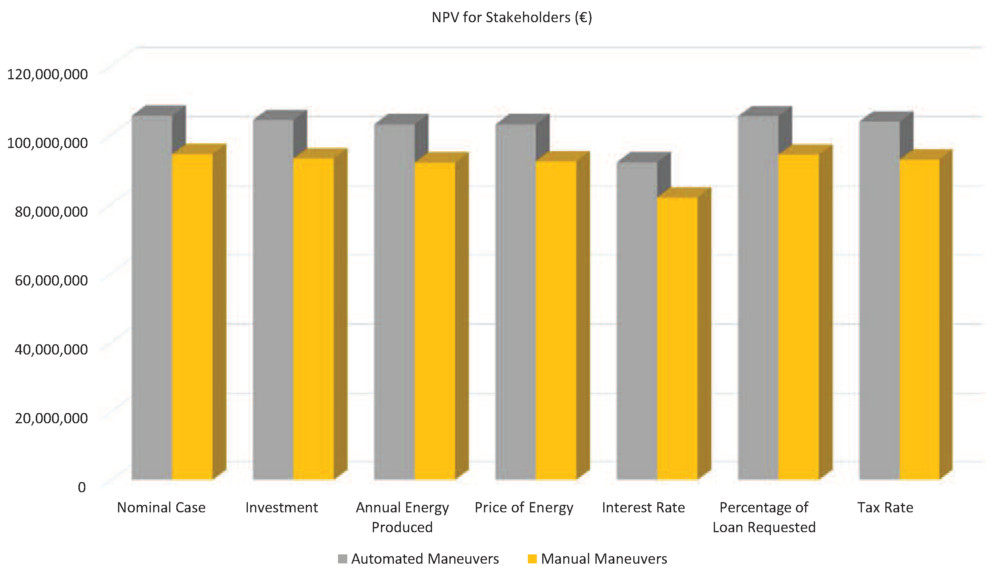
4.2.2. Sensitivity Analysis

After determining those parameters that could have an effect on the profitability of the project (Section 3.5), we shall now identify those that are most critical for the project. The means employed to determine the significance of the aforementioned parameters in the case of the feasibility of the project will be that of altering their values to a slight extent, after which the variations that occur for the reference values considered will be studied. These will, in this case, be the NPV, the IRR and the DPBP of the stakeholders and the project. We shall consider those parameters that lead to higher variations in the references in question to be critical values. In this line of action, the following scenarios have been taken into consideration: (i) an increase in the initial investment to 1%; (ii) a decrease in the AEP by the TEF to 1%; (iii) a decrease in the price of energy to 1%; (iv) an increase in the interest rate to 1%; (v) a decrease in the percentage of the loan requested to 1%; and (vi) an increase in the tax rate to 1%. The values obtained for the nominal case for manual values are the following: the NPV for the project is 64,066,094 € and the NPV for the stakeholders is 94,399,360 €; the IRR for the project is 8.126% and the IRR for the stakeholders is 24.17%, and the DPBP for the project is 13.04 years and the DPBP for the stakeholders is 4.95 years. The values obtained for the nominal case for automated maneuvers are, meanwhile, the following: the NPV for the project is 75,432,173 € and the NPV for the stakeholders is 105,494,103 €; the IRR for the project is 8.21% and the IRR for the stakeholders is 24.17%, and the DPBP for the project is 12.23 years and the DPBP for the stakeholders is 4.37 years. Figure 18 and Figure 19 depict the results of the NPV sensitivity analysis with regard to the project and the stakeholders when manual and automated maneuvers are carried out, while

Table 2. Sensitivity analysis results when manual and automated maneuvers are carried out.

	Manual Maneuvers
	Project			Stakeholders
	${∆}_{NPV}$	${∆}_{IRR}$	${∆}_{DPBP}$	${∆}_{NPV}$	${∆}_{IRR}$	${∆}_{DPBP}$
Investment is increased to 1%	–2.46%	–1.66%	1.23%	–1.29%	–2.0%	2.49%
Annual energy produced by the farm decreases to 1%	–3.82%	–1.84%	1.38%	–2.52%	-2.23%	2.79%
Price of the energy decreases to 1%	–3.14%	–1.52%	1.13%	–2.07%	–1.83%	2.28%
Interest rate increases to 1%	–28.56%	∼0%	7.88%	–13.21%	∼0%	3.09%
Percentage of the loan requested decreases to 1%	–0.34%	–0.20%	0.17%	–0.17%	-1.40%	3.61%
Tax rate increases to 1%	–2.41%	–0.20%	0.78%	–1.57%	–1.40%	1.35%
	Automated Maneuvers
	Project			Stakeholders
	${∆}_{NPV}$	${∆}_{IRR}$	${∆}_{DPBP}$	${∆}_{NPV}$	${∆}_{IRR}$	${∆}_{DPBP}$
Investment is increased to 1%	–2.06%	–1.64%	1.22%	–1.18%	–2.0%	2.33%
Annual energy produced by the farm decreases to 1%	–3.28%	–1.84%	1.32%	–2.34%	–2.23%	1.69%
Price of the energy decreases to 1%	–3.27%	–1.52%	1.32%	–2.34%	–1.83%	2.49%
Interest rate increases to 1%	–25.45%	∼0%	7.36%	–12.76%	∼0%	2.77%
Percentage of the loan requested decreases to 1%	–0.29%	–0.18%	0.16%	–0.15%	–1.41%	3.6%
Tax rate increases to 1%	–2.25%	–0.18%	0.82%	–1.61%	–1.41%	1.35%

shows the variations in the NPV, IRR and DPBP of the project and the stakeholders as regards manual and automated maneuvers in the aforementioned scenarios.

These results allow us to conclude that, in the nominal case, the TEP carried out using manual and automated maneuvers are economically feasible, with a higher profitability for automated maneuvers. Furthermore, both the automated and the manual maneuvers are affected by the same parameters as those that affect the profitability of the project, which are the variations in interest rate, the price of energy and the AEP. This is owing to the fact that these parameters concern the financing of the farm, and the incomes will be achieved during the entire service life of the project. The profitability of the project is, however, less affected by the variations related to the tax rate, the percentage of the loan requested and the investment.

4.3. Comparative Sensitivity Analysis

Having employed a case study to demonstrate the excellent profitability and economic feasibility as regards the use of both manual and automated maneuvers, we shall now develop a comparative sensitivity analysis in order to quantify, in an economic manner, how much better the use of automated maneuvers is with regard to the use of manual maneuvers. As occurred in Section 4.2.2, we shall study the following scenarios: (i) the nominal case; (ii) an increase in the initial investment to 1%; (iii) a decrease in the AEP by the TEF to 1%; (iv) a decrease in the price of energy to 1%; (v) an increase in the interest rate to 1%; (vi) a decrease in the percentage of the loan requested to 1%; and (vii) an increase in the tax rate to 1%.

Table 3. Comparative sensitivity analysis results for the use of automated maneuvers when compared to the use of manual maneuvers.

	Project			Stakeholders
	${∆}_{NPV}$	${∆}_{IRR}$	${∆}_{DPBP}$	${∆}_{NPV}$	${∆}_{IRR}$	${∆}_{DPBP}$
Nominal Case	17.74%	∼0%	−6.23%	11.75%	∼0%	−11.45%
Investment is increased to 1%	18.24%	∼0%	−6.23%	11.94%	∼0%	−11.74%
Annual energy produced by the farm decreases to 1%	18.39%	∼0%	−6.25%	12.03%	∼0%	−11.84%
Price of the energy decreases to 1%	17.58%	∼0%	−6.02%	11.52%	∼0%	−11.41%
Interest rate increases to 1%	22.88%	∼0%	−6.64%	12.40%	∼0%	−11.86%
Percentage of the loan requested decreases to 1%	18.48%	∼0%	−6.51%	11.77%	∼0%	−11.46%
Tax rate increases to 1%	17.93%	∼0%	−6.16%	11.78%	∼0%	−11.60%

shows the results of the comparative sensitivity analysis carried out for the variations in the NPV, IRR and DPBP of the project and the stakeholders in the case of the use of automated maneuvers when compared to the use of manual maneuvers in the aforementioned scenarios. These results allow us to conclude that the profitability of the case study is higher and the investment is recovered faster when using automated maneuvers for all scenarios, demonstrating that, from an economic point of view, this is an attractive solution as regards a future commercialization of these devices.

5. Conclusions and Future Works

The development of improved installation and maintenance procedures for technologies that harness energy from ocean currents is a promising research field that needs to be studied in detail in order to achieve a successful future commercialization of these technologies. In this paper, we have explained the procedures for manual and automated installation and maintenance maneuvers for gravity-based first generation TECs, and have also carried out an economic-financial evaluation in order to highlight the merits of automated installation and maintenance maneuvers for tidal energy technologies. Some of the potential benefits that the use of these maneuvers could provide are the following: (i) an increase in the competitiveness of these technologies; (ii) a reduction in human resources and the number and duration of installation and maintenance operations; (iii) the use of cheaper general purpose ships instead of high cost special vessels for maintenance operations; and (iv) a higher project profitability, among others. We have conducted a numerical case study of a TEF in the Alderney Race (UK). This farm comprises 42 TECs of 1.2 MW, and the study was carried out with the objective of determining the economic-financial viability of the project when employing either automated or manual installation and maintenance maneuvers. After applying the economic-financial procedure explained throughout this paper to the case study, we attained results indicating that the project would, in both cases, obtain a good profitability and can consequently recommend investment from both accounting and financial points of view, since the benefits produced from the first year are good. We have additionally discovered that the profitability is even greater when employing devices capable of performing automated maneuvers. The aforementioned results also indicate that the variables that have the greatest influence on the profitability of the project are, in the case of both types of maneuvers, the AEP, the price of energy and the interest rate. Finally, having attained the results of the case study, we can conclude that the economic-financial methodology employed is useful as regards modeling different renewable energy projects, as is also the case of the manual and automated installation and maintenance procedures for first generation TECs presented in this work. This methodology additionally has an advantage in that it could, with minor adaptations, be used for other kinds of offshore renewable energy projects and TEC designs. Our future research will be focused on the application of this model to other offshore renewable energy projects.

References

1. Rodríguez-Delgado, C.; Bergillos, R.A.; Iglesias, G. Dual wave farms for energy production and coastal protection under sea level rise. J. Clean. Prod. 2019, 222, 364–372. [Google Scholar] [CrossRef]
2. Atilgan, B.; Azapagic, A. Life cycle environmental impacts of electricity from fossil fuels in Turkey. J. Clean. Prod. 2015, 106, 555–564. [Google Scholar] [CrossRef]
3. Sequeira, T.N.; Santos, M.S. Renewable energy and politics: A sistematic review and new evidence. J. Clean. Prod. 2018, 192, 553–568. [Google Scholar] [CrossRef]
4. Sinha, A.; Shahbaz, M.; Sengupta, T. Renewable energy and policies and contratictions in causality: A case of next 11 countries. J. Clean. Prod. 2018, 197, 73–84. [Google Scholar] [CrossRef]
5. Directive 2009/28/EC of the European Parliament and of the Council of 23 April 2009 on the promotion of the use of energy from renewable sources and amending and subsequently repealing directives 2001/77/EC and 2003/30/EC. Off. J. Eur. Union 2009, 16–60.
6. Magagna, D.; MacGillivray, A.; Jeffrey, H.; Hanmer, C.; Raventos, A.; Badcock-Broe, A.; Tzimas, E. Wave and Tidal Energy Strategic Technology Agenda; SI Ocean: Brussels, Belgium, 2014. [Google Scholar]
7. Jeffrey, H.; Jay, B.; Winskel, M. Accelerating the development of marine energy: Exploring the prospects, benefits and challenges. Technol. For. Soc. Chang. 2013, 80, 1306–1316. [Google Scholar] [CrossRef]
8. United Nations Framework Convention on Climate Change, 2015. Paris Agreement; UNFCCC Secretariat: Bonn, Germany, 2016. [Google Scholar]
9. Overcoming Research Challenges for Ocean Renewable Energy; Energy Research Knowledge Centre: Brussels, Belgium, 2013.
10. Ocean Energy Strategic Roadmap 2016, Building Ocean Energy for Europe. Ocean Energy Forum, 8 November 2016.
11. Hardisty, J. The Analysis of Tidal Stream Power; Wiley: Hoboken, NJ, USA, 2009; ISBN 978-0-470-72451-4. [Google Scholar]
12. Portilla, M.P.; Somolinos, J.A.; López, A.; Morales, R. Modelado dinámico y control de un dispositivo sumergido provisto de actuadores hidrostáticos. Revista Iberoamericana de Automática e Informática Industrial 2018, 15, 12–23. [Google Scholar] [CrossRef]
13. Alstom Tidal Turbines Web Page. Available online: https://marineenergy.biz/tag/alstom/ (accessed on 3 April 2019).
14. Andritz Hydro Hammerfest. How It Works. Available online: http://www.andritz.com/hy-hammerfest.pdf (accessed on 3 April 2019).
15. Fallon, D.; Hartnett, M.; Olbert, A.; Nash, S. The effects of array configuration on the hydro-environmental impacts on tidal turbines. Renew. Energy 2014, 64, 10–25. [Google Scholar] [CrossRef]
16. Segura, E.; Morales, R.; Somolinos, J.A. A strategic analysis of tidal current energy conversion systems in the European Union. Appl. Energy 2018, 212, 527–551. [Google Scholar] [CrossRef]
17. Denny, E. The economics of tidal energy. Energy Policy 2009, 37, 1914–1924. [Google Scholar] [CrossRef]
18. Segura, E.; Morales, R.; Somolinos, J.A.; López, A. Techno-economic challenges of tidal energy conversion systems: Current status and trends. Renew. Sustain. Energy Rev. 2017, 77, 536–550. [Google Scholar] [CrossRef]
19. Segura, E.; Morales, R.; Somolinos, J.A. Cost assessment methodology and economic viability of tidal energy projects. Energies 2017, 10, 1806. [Google Scholar] [CrossRef]
20. Nautricity Web Page. 2016. Available online: http://www.nautricity.com/cormat/ (accessed on 3 April 2019).
21. Tocardo Web Page. 2016. Available online: http://www.tocardo.com/ (accessed on 3 April 2019).
22. Somolinos, J.A.; López, A.; Portilla, M.P.; Morales, R. Dynamic model and control of a new underwater three-degree-of-freedom tidal energy converter. Math. Probl. Eng. 2015, 2015, 948048. [Google Scholar] [CrossRef]
23. López, A.; Somolinos, J.A.; Núñez, L.R.; Morales, R. Dynamic Model and Experimental Validation for the Control of Emersion Maneuvers of Devices for Marine Currents Harnessing. Renew. Energy 2017, 103, 333–345. [Google Scholar]
24. Morales, R.; Fernández, L.; Segura, E.; Somolinos, J.A. Maintenance Maneuver Automation for an Adapted Cylindrical Shape TEC. Energies 2016, 9, 746. [Google Scholar] [CrossRef]
25. Fernández, L.; Segura, E.; Portilla, M.P.; Morales, R.; Somolinos, J.A. Dynamic model and nonlinear control for a two degrees of freedom first generation tidal energy converter. IFAC-PapersOnLine 2016, 49–23, 373–379. [Google Scholar] [CrossRef]
26. Castro-Santos, L.; Filgueira-Vizoso, A.; Lamas-Galdo, I.; Carral-Couce, L. Methodology to calculate the installation costs of offshore wind farms located in deep waters. J. Clean. Prod. 2018, 170, 1124–1135. [Google Scholar] [CrossRef]
27. Castro-Santos, L.; Silva, D.; Rute Bento, A.; Salvaçao, N.; Guetes Soares, C. Economic Feasibility of Wave Energy Farms in Portugal. Energies 2018, 11, 3149. [Google Scholar] [CrossRef]
28. Castro-Santos, L.; Martins, E.; Guedes-Soares, C. Cost assessment methodology for combined wind and wave floating offshore renewable energy systems. Renew. Energy 2016, 97, 866–880. [Google Scholar] [CrossRef]
29. Castro-Santos, L.; Martins, E.; Guedes-Soares, C. Economic comparison of technological alternatives to harness offshore wind and wave energies. Energy 2017, 140, 1121–1130. [Google Scholar] [CrossRef]
30. Voith. Tidal Current Power Stations. Available online: http://voith.com/en/productsservices/hydro-power/ocean-energies/tidal-current-power-stations--591.html (accessed on 3 April 2019).
31. Tidal Energy: Technology Brief. International Renewable Energy Agency (IRENA). June 2014. Available online: https://www.irena.org/documentdownloads/publications/tidal_energy_v4_web.pdf (accessed on 4 April 2019).
32. BVG Associates. A Guide to an Offshore Wind Farm. The Crown Estate. 2010. Available online: http://www.thecrownestate.co.uk/media/5408/ei-a-guide-to-an-offshore-wind-farm.pdf (accessed on 4 April 2019).
33. TradeWinds. The Global Shipping News Source. 2017. Available online: http://www.tradewindsnews.com/ (accessed on 4 April 2019).
34. Altlantis Resources. AR1000. 2017. Available online: https://www.atlantisresourcesltd.com/services/turbines/ (accessed on 4 April 2019).
35. ABR Company Ltd. International Tug & OSV, Incorporating Salvage News. 2017. Available online: https://www.tugandosv.com/about_the_magazine.php (accessed on 4 April 2019).
36. Somolinos, J.A. Control de operaciones de dispositivos marinos de aprovechamiento de la energía hidrocinética. Proyecto RETOS de la Sociedad DPI2014m bn-53499-R. 2015. Available online: http://www.upm.es/observatorio/vi/index.jsp?pageac=grupo.jsp&idGrupo=391 (accessed on 20 May 2019).
37. Espín, M. Modelado Dinámico y Control de Maniobras de Dispositivos Submarinos. Ph.D. Thesis, ETSIN-UPM, Madrid, Spain, 2015. [Google Scholar]
38. Sánchez, G. Diseño de un dispositivo para el aprovechamiento de la energía de las corrientes (DAEC) y su integración en un parque marino. Master’s Thesis, Escuela Técnica Superior de Ingenieros Navales, Universidad Politécnica de Madrid (ETSIN-UPM), Madrid, Spain, 2014. [Google Scholar]
39. Subsea Power Cables in Shallow Water Renewable Energy Applications. Det Norske Veritas (DNV) AS. February 2014. Available online: https://rules.dnvgl.com/docs/pdf/DNV/codes/docs/2014-02/RP-J301.pdf (accessed on 29 May 2019).
40. Bryden, I.G.; Couch, S.J. ME1–Marine energy extraction: Tidal resource analysis. Renew. Energy 2006, 31, 133–139. [Google Scholar] [CrossRef]
41. Charlier, R.H. A Sleeper awakes: Tidal current power. Renew. Sustain. Energy Rev. 2003, 7, 515–529. [Google Scholar] [CrossRef]
42. Marine Current Turbines (MCT). An Atlantis Company. Tidal Energy Section. 2017. Available online: http://www.marineturbines.com/Tidal-Energy (accessed on 4 April 2019).
43. López, A.; Somolinos, J.A.; Núñez, L.R. Dispositivo para el aprovechamiento de las corrientes marinas multi-rotor con estructura poligonal. Patent Number P201430182. ES2461440, 25 November 2014. [Google Scholar]
44. López, A.; Somolinos, J.A.; Núñez, L.R. Underwater electrical generator for the harnessing of bidirectional flood currents. U.S. Patent Application 12/978993, 30 June 2011. [Google Scholar]
45. López, A.; Núñez, L.R.; Somolinos, J.A. Generador electrico submarino para el aprovechamiento de las corrientes de flujo bidireccional. Patent Number ES 2341311, 30 December 2009. [Google Scholar]
46. Segura, E.; Morales, R.; Somolinos, J.A. Economic-Financial Modeling for Marine Current Harnessing Projects. Energy 2018, 158, 859–880. [Google Scholar] [CrossRef]
47. Delogu, M.; Zanchi, L.; Maltese, S.; Boloni, A.; Pierini, M. Environmental and economic life cycle assessment of a lightweight solution for an automotive component: A comparison between talc-filled and hollow glass microspheres-reinforced polymer composites. J. Clean. Prod. 2016, 139, 548–560. [Google Scholar] [CrossRef]
48. IEC 60300-3-3:2004 - Dependability Management - Part 3-3: Application Guide - Life Cycle Costing; IEC: Geneva, Switzerland, 2004.
49. Dhillon, B.S. Life-Cycle Costing for Engineers; CRC Press: Boca Raton, FL, USA, 2010. [Google Scholar]
50. Vail Farr, J. Systems Life Cycle Costing—Economic Analysis, Estimation and Management; CRC Press: Boca Raton, FL, USA, 2011. [Google Scholar]
51. Hirt, G.; Block, S. Fundamentals of Investment Management, 10th ed.; McGraw-Hill Education: New York, NY, USA, 2011. [Google Scholar]
52. Kimmel, P.D.; Weygandt, J.J.; Kieso, D.E. Accounting: Tools for Business Decision Making, 4th ed.; John Wiley & Sons Ltd: Hoboken, NJ, USA, 2011. [Google Scholar]
53. Wild, J.J. Financial Accounting Fundamentals, 6th ed.; McGraw-Hill Education: New York, NY, USA, 2017. [Google Scholar]
54. Short, W.; Packey, D.; Holt, T. A Manual for the Economic Evaluation of Energy Efficiency and Renewable Energy Technologies; NREL/TP-462-5173; National Renewable Energy Laboratory: Colorado, CO, USA, 1995.
55. Det Norske Veritas AS. Det Norske Veritas (DNV), DNV–OS–J101. Design of Offshore Wind Turbine Structures; Det Norske Veritas AS.: Oslo, Norway, 2010; pp. 1–142. [Google Scholar]
Figure 1. Installation sequence at tidal farm level: (a) joining the umbilical cable to the platform by means of a cable-laying vessel; (b) umbilical cable-laying process; (c) connection of the umbilical cable to the TEC (Tidal Energy Converter) structure; and (d) cable-laying process of the next umbilical cable.
Energies 12 02464 g001
Figure 2. Installation of the submarine cables: (a) installation of the base; (b) ROV (Remotely Operated Vehicle) performing the trenching process of the first umbilical cable; (c) ROV starting umbilical cable burial process; and (d) ROV finishing the burying process of the umbilical cable.
Energies 12 02464 g002
Figure 3. Example of TEC used for manual installation and maintenance maneuvers. Additional details about this TEC design can be found in [38].
Energies 12 02464 g003
Figure 4. Installation of the structure of the TECs: (a) position required to install the base; (b) connection of the umbilical cables to the TEC structure; (c) controlled descent of the TEC structure; (d) fixing the TEC structure to the seabed; (e) placement of the concrete ballasts; and (f) installation of the TEC structure once the process has been completed.
Energies 12 02464 g004
Figure 5. Installation of the gondola of the TECs: (a) cable-recovery process; (b) connection of the cables to the tool in charge of lowering the gondola; (c) controlled descent of the gondola; (d) process of inserting the gondola into the TEC structure; (e) tool and cable removal process; and (f) end of gondola-installation process.
Energies 12 02464 g005
Figure 6. Tool used for manual installation and maintenance maneuvers (installation and recovery of the gondola).
Energies 12 02464 g006
Figure 7. Maintenance operations of the gondola: (a) positioning the special vessel above the gondola; (b) descent process of the tool; (c) coupling process between the tool and the gondola and cable tensioning process; (d) activation of the hydraulic system of the tool to fix it to the gondola; (e) gondola lifting process; and (f) gondola recovered.
Energies 12 02464 g007
Figure 8. First generation TEC designed for automated maneuvers: (a) shape of the gondola and (b) distribution equipment.
Energies 12 02464 g008
Figure 9. Automated installation maneuver of the gondola (immersion sequence): (a) movement of the device with maneuver control in closed loop; (b) connection between the cable wire and the gondola; (c) immersion maneuver in closed loop; (d) immersion maneuver in closed loop (cont.); (e) immersion maneuver finished; and (f) installation maneuver in closed loop finalized.
Energies 12 02464 g009
Figure 10. Automated maintenance maneuver of the gondola (emersion sequence): (a) the water begins to be emptied out of the gondola; (b) separation between the TEC structure and the gondola and start of emersion process; (c) emersion maneuver in closed loop; (d) emersion maneuver in closed loop (cont.); (e) emersion maneuver finalized, the inner ballasts are completely empty and are disconnected from the control system; and (f) start of maintenance tasks.
Energies 12 02464 g010
Figure 11. Economic-financial model for gravity-based tidal energy projects.
Energies 12 02464 g011
Figure 12. Life cycle costs for tidal energy projects composed of gravity-based first generation TECs.
Energies 12 02464 g012
Figure 13. How annual sales are computed: A summary.
Energies 12 02464 g013
Figure 14. Proposed TEF: (a) view and; (b) configuration.
Energies 12 02464 g014
Figure 15. Energy generated by TECs placed in the rows of the TEF.
Energies 12 02464 g015
Figure 16. Comparative financial ratios for manual and automated maneuvers: (a) solvency ratio (SR), and (b) total debt ratio (TDR).
Energies 12 02464 g016
Figure 17. Comparative economic ratios for manual and automate maneuvers: (a) return of assets (ROA), and (b) return of equity (ROE).
Energies 12 02464 g017
Figure 18. NPV (Net Present Value) results of the project when manual and automated maneuvers are carried out.
Energies 12 02464 g018
Figure 19. NPV results for the stakeholders when manual and automated maneuvers are carried out.
Energies 12 02464 g019