Improving Performance of Simplified Computational Fluid Dynamics Models via Symmetric Successive Overrelaxation

Abstract

The ability to model fluid flow and heat transfer in process equipment (e.g., shell-and-tube heat exchangers) is often critical. What is more, many different geometric variants may need to be evaluated during the design process. Although this can be done using detailed computational fluid dynamics (CFD) models, the time needed to evaluate a single variant can easily reach tens of hours on powerful computing hardware. Simplified CFD models providing solutions in much shorter time frames may, therefore, be employed instead. Still, even these models can prove to be too slow or not robust enough when used in optimization algorithms. Effort is thus devoted to further improving their performance by applying the symmetric successive overrelaxation (SSOR) preconditioning technique in which, in contrast to, e.g., incomplete lower–upper factorization (ILU), the respective preconditioning matrix can always be constructed. Because the efficacy of SSOR is influenced by the selection of forward and backward relaxation factors, whose direct calculation is prohibitively expensive, their combinations are experimentally investigated using several representative meshes. Performance is then compared in terms of the single-core computational time needed to reach a converged steady-state solution, and recommendations are made regarding relaxation factor combinations generally suitable for the discussed purpose. It is shown that SSOR can be used as a suitable fallback preconditioner for the fast-performing, but numerically sensitive, incomplete lower–upper factorization.

1. Introduction

In engineering practice, it is often the case that process equipment is designed according to various rules of thumb. No optimization is generally done and, at best, a single computational fluid dynamics (CFD) simulation is carried out to verify that the design meets the key requirements of the future operator of the apparatus. This means that suboptimal designs or solutions, potentially leading to operating problems, are not uncommon.

One of the ways to remedy the situation is to use simplified CFD models. In spite of them not being as accurate as the standard CFD models, it has been shown [1] that they can provide useful quantitative information. What is more, these models feature significantly shorter computational times and their application in optimization algorithms is therefore much less cumbersome. To obtain solutions even faster, however, the numerical methods used to solve the underlying linear systems of equations can also be preconditioned. This means that instead of solving the original linear system

Ax = b,

(1)

where A is the coefficient matrix, x the solution vector, and b the right-hand side vector, one considers the system

M⁻¹Ax = M⁻¹b.

(2)

here, M denotes the preconditioning matrix such that M⁻¹A has a smaller condition number than A and, therefore, linear system (2) features better convergence. It should also be noted that M⁻¹A often is not formed explicitly but, instead, Mu = v is solved for various auxiliary vectors u and v within the numerical solution method itself.

There are many different preconditioning techniques (i.e., ways to choose M) available, and the selection of the best one for a particular purpose depends mainly on the type of equation that is being solved and the employed ordering of the variables. However, the most commonly used techniques are likely various flavors of incomplete lower–upper factorization (ILU) [2] (these were numerically investigated by Chapman et al. [3]) and symmetric successive overrelaxation (SSOR) [4]. Although SSOR was originally intended for symmetric matrices, it was shown [5] to also work when the matrices are not symmetric. Assuming the splitting A = D + L + U, where D is the diagonal of A and L and U its strictly lower and upper triangular parts, respectively, the SSOR preconditioning technique is applied within the numerical solution method as two SOR sweeps using different values of ω. The iteration process for auxiliary vectors u, v (depend on the actual solution method used) can then be written as

u^{(k + 1/2)} = (D + ω_FL)⁻¹[(1 − ω_F)D − ω_FU]u^(k) + ω_F(D + ω_FL)⁻¹v (forward sweep)
u^{(k + 1)} = (D + ω_RU)⁻¹[(1 − ω_R)D − ω_RL]u^{(k + 1/2)} + ω_R(D + ω_RU)⁻¹v, (backward sweep)

(3)

where ω_F and ω_R denote the corresponding forward and backward relaxation factors. In other words, direct application of the inverse of the preconditioning matrix, M⁻¹, is replaced by preconditioned fixed point iteration.

The advantages of SSOR are evidenced by the existence of a multitude of papers discussing improved versions of this technique or its extensions to various specific applications. Bai [6] studied SSOR-like preconditioners for non-Hermitian positive definite linear systems, for which the respective matrix was either Hermitian-dominant or skew–Hermitian-dominant. The paper also discussed the results of numerical implementations, showing that Krylov subspace iteration methods, when accelerated using SSOR-like preconditioners, are efficient solvers for classes of non-Hermitian positive definite linear systems. A “shifted” version of SSOR for non-Hermitian positive definite linear systems with a dominant Hermitian part was proposed by Tan [7]. Zhang [8], on the other hand, introduced an SSOR-like preconditioner for saddle point problems with a dominant skew-Hermitian part. A class of hybrid preconditioning methods for accelerated solution of saddle point problems was discussed by Wang [9], while Chen et al. [10] proposed a version of SSOR suitable for preconditioning of large dense complex linear systems arising from three-dimensional electromagnetic scattering. Wu and Li [11] introduced a modified SSOR technique for the solution of Helmholtz equations.

Preconditioning can also be done block-wise. This was discussed, e.g., by Zhang and Cheng [12] in terms of large sparse saddle point problems, and by Huang and Lu [13], who focused on SSOR block preconditioners applied in image restoration. Because, in fact, preconditioning means obtaining an easily invertible approximation of the original matrix, one can also use SSOR for just this purpose as shown, for example, by Meng et al. [14] in the context of fast recovery of density 3D data from gravity data. Similarly, a massively-parallel GPU implementation of the conjugate gradient method, which uses the approximate inverse matrix derived from SSOR as the preconditioning matrix, was proposed by Helfenstein and Koko [15].

Performance comparisons of SSOR and other, simpler preconditioning techniques were presented, e.g., by Meyer [16], who focused on genomic evaluation and by Sanjuan et al. [17], who used SSOR to accelerate parallel wind field calculations. In the latter paper, the authors also evaluated a new, reordered sparse matrix storage format and showed that this format can markedly shorten computational time. This confirms the earlier findings of Duff and Meurant [18], who investigated the effect of ordering on the convergence of the conjugate gradient method preconditioned, among others, using SSOR, or DeLong and Ortega [19], who focused on parallel implementations of SOR in terms of natural and multicolor orderings. Chen et al. [20], on the other hand, proposed a novel reordering technique for SSOR approximate inverse preconditioner, used together with a GPU-accelerated conjugate gradient solver, which should maximize the coalescing of global memory accesses.

Many SSOR-like, a priori preconditioned numerical solution methods using different splittings of the coefficient matrix have also been proposed for various types of problems. A three-parameter extension of the SSOR method intended for singular saddle point problems, which commonly arise, e.g., in fluid dynamics, was proposed by Li and Zhang [21]. A differently accelerated generalized three-parameter method for both singular and non-singular problems was introduced by Pan [22]. Similarly, a three-parameter unsymmetric SOR method for such saddle point problems was proposed, for example, by Liang and Zhang [23], who also discussed the choice of optimal values of the parameters. Many different SSOR-like methods are available for augmented systems, as well. Wang and Huang [24] introduced a four-parameter method, Louka and Missirlis [25] introduced a five-parameter extrapolated form of SSOR, and Najafi and Edalatpanah [26] introduced an improved version of the modified SSOR method for large sparse augmented systems, proposed earlier by Darvishi and Hessari [27]. Another improved SSOR method intended for the solution of augmented systems was proposed by Salkuyeh et al. [28]. In the case of complex systems, one can use, for instance, the accelerated method by Huang et al. [29], that is, an accelerated version of the method by Edalatpour et al. [30], in which the solution vector is split into two subvectors and different relaxation factors are used when solving for each of them. Likewise, one can employ the preconditioned variant of the generalized SSOR method by Hezari et al. [31] or the method by Salkuyeh et al. [32], which solves a real system obtained from the original, complex one. Block linear systems can be solved, e.g., using the block-preconditioned SSOR method by Pu and Wang [33].

The majority of the papers mentioned above discuss convergence (or at least semi-convergence) of the proposed methods, and many also include some information on the optimal selection of the relaxation factors. Kushida [34] focused on the estimation of convergence of the original SSOR preconditioner via a condition number, while general discussion related to SSOR-like methods for non-Hermitian positive definite linear systems was published in [35]. Augmented systems were addressed, for example, by Wang and Huang [36]. Similarly, there are papers focusing on convergence and optimal selection of the relaxation factors in the case of methods for block 2 × 2 linear systems [37], saddle point problems [38], parallel SSOR implementations [39], the Poisson equation [40], etc. In all these cases, however, convergence was investigated via spectral analysis, which is often prohibitively expensive [41]. The present paper, focusing on fast estimation of suitable SSOR relaxation factors in engineering practice, therefore, investigates the convergence experimentally using several different simplified 3D CFD flow models. The suitability of specific combinations of relaxation factors is assessed on the basis of mean computational times needed to reach converged steady-state solutions. The best-performing combinations of relaxation factors are then given together with the obtained relaxation factor trends.

2. Materials and Methods

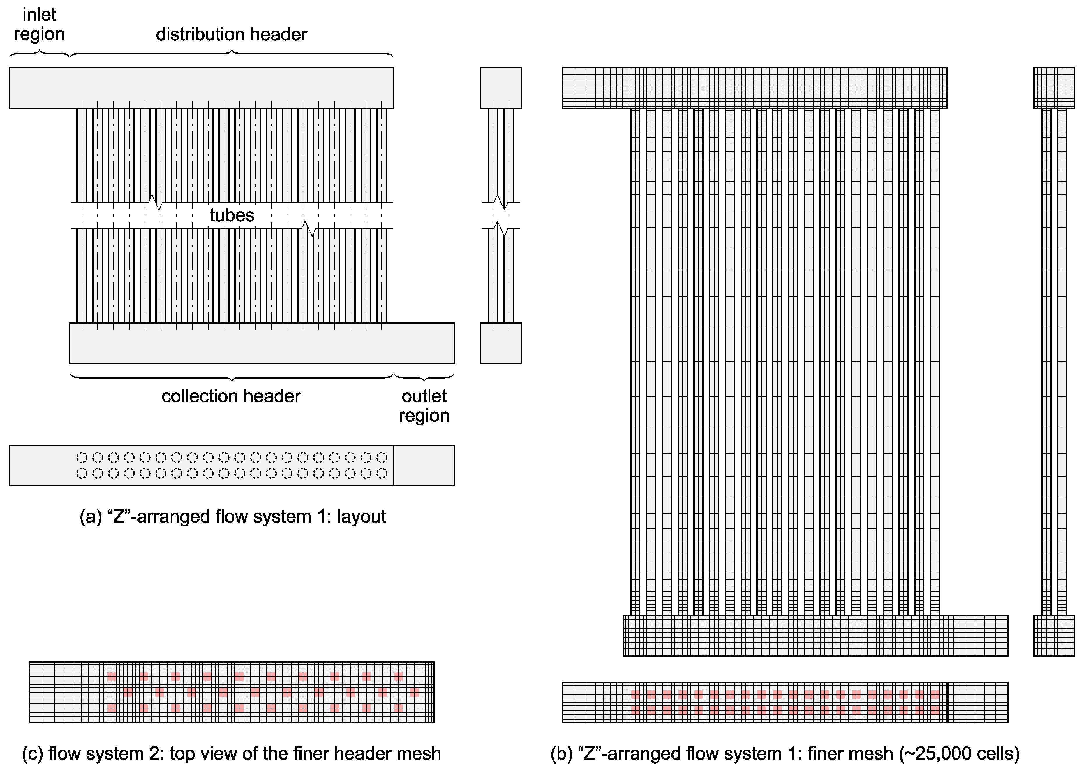
Three different flow systems, with both the “U” and the “Z” flow arrangements (“U”: outlet on the same side of the flow system as the inlet, “Z”: outlet on the opposite side), were used to generate test cases. Moreover, in two of these three flow systems, the mesh fineness was also varied (coarser and finer mesh). This yielded ten flow system configurations in total, with simplified, cuboid cell-only meshes of different sizes ranging from ~6000 cells to ~41,000 cells (see

Table 1. Flow system parameters: W, L, and H denote width, length, and height, respectively, p_r row pitch, and p_t tube pitch.

Parameter	Flow System 1	Flow System 2	Flow System 3
Headers (W × L × H)	40 × 320 × 40 mm	60 × 340 × 60 mm	100 × 340 × 100 mm
Inlet/outlet region (L)	60 mm	60 mm	60 mm
Tube bundle	2 inline rows, 20 tubes/row, pr = pt = 15.6 mm	3 staggered rows (45°), 10 tubes/row, pr = 15.6 mm, pt = 2pr	5 staggered rows (45°), 10 tubes/row, pr = 15.6 mm, pt = 2pr
Tubes	⌀10 mm × 500 mm	⌀10 mm × 500 mm	⌀10 mm × 500 mm
Flow arrangement	“U” or “Z”	“U” or “Z”	“U” or “Z”
Mesh	coarser: ~6000 cells, finer: ~25,000 cells	coarser: ~8000 cells, finer: ~41,000 cells	coarser: ~16,000 cells

). The meshes were generated automatically by the employed benchmarking software (see further) using the key parameters listed in Table 1. Due to the cuboid nature of the meshes, cell sizes were, in all computational domains, governed primarily by how many cell faces comprised a tube cross section (coarser mesh: 1 face only, finer mesh: 2 × 2 faces) and by the utilized cell growth factor. Sample meshes are shown in Figure 1.

As for boundary conditions, 0.5 kg/s of water at 300 K was fed into the inlet while pressure at the outlet was set to 101,325 Pa. All walls were adiabatic except for tube walls, where a specific heat flux of 15 kW/m² was set when the energy equation was enabled. Steady state simulations were carried out using the same CFD setup as in [42], that is, the SIMPLEC pressure-velocity coupling [43] was employed together with the Power Law discretization scheme [44]. Standard scaled residual limits, i.e., 10⁻³ for continuity and momentum and 10⁻⁶ for energy, were used. Only the natural ordering of the variables was considered in this study.

The SSOR preconditioning technique was paired with two widely used numerical solution methods, which were shown by an earlier study [42] to perform very well in simplified 3D CFD models. The conjugate gradient (CG) numerical solution method [45] was employed in the pressure correction equation. The momentum and energy equations, on the other hand, were solved using the bi-conjugate gradient stabilized numerical method with the minimization of residuals over L-dimensional subspaces (BiCGstab(L)) [46], with L = 1, 2, or 3. Performance of the ILU preconditioner (which is efficient, but the construction of the respective preconditioning matrix may not always be possible) was taken as the baseline.

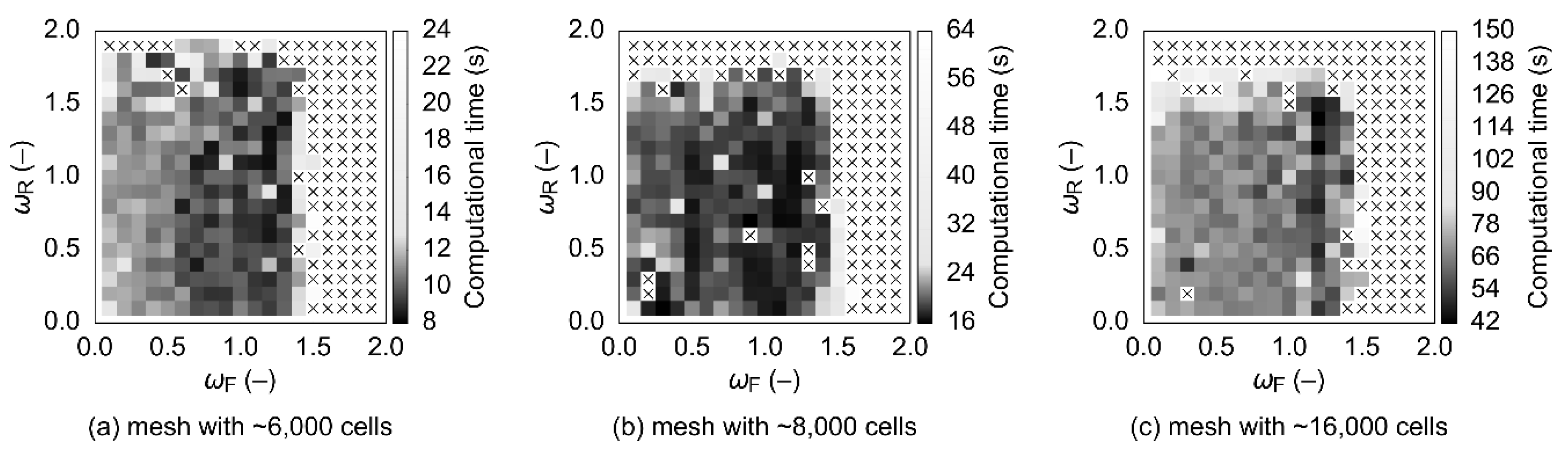
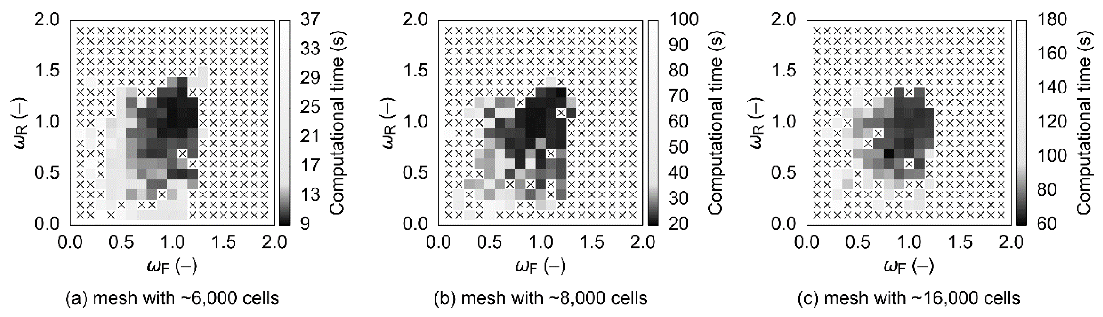
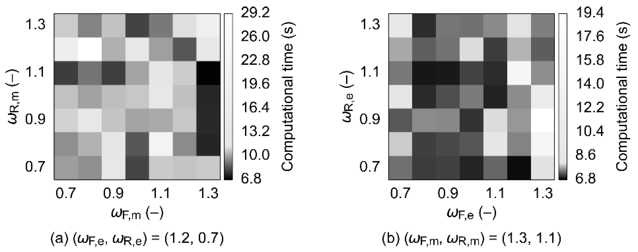
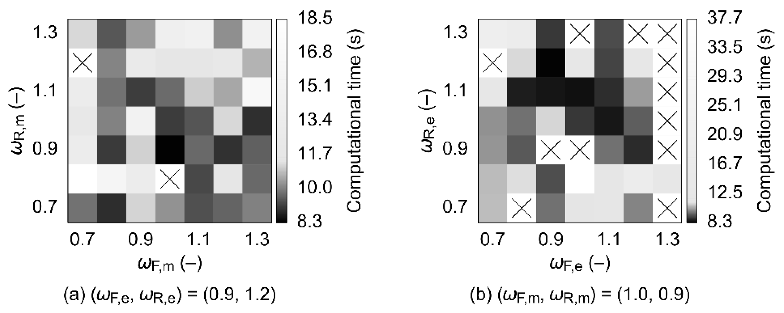
The SSOR-preconditioned numerical solution methods were tested with various tuples of ω_F, ω_R = 0.1, 0.2, …, 1.8, 1.9 in successive steps, depending on the obtained results. Promising combinations of ω_F and ω_R were then taken as pivots, and their square neighborhoods were tested further—that is, all combinations of ω_F, ω_R with the respective values being ω – 0.04, ω – 0.02, ω, ω + 0.02, and ω + 0.04 were evaluated except for the original pivot point (ω_F, ω_R). In order to be able to compare SSOR to the baseline (ILU), all the ten meshes were also evaluated using the ILU-preconditioned combinations of solution methods. In total, 50,620 CFD model setups were tested.

The same benchmarking simplified 3D CFD Java software application was used as in [42], and, therefore, the reader is kindly referred to this paper for details (please note that the software is not publicly available). The benchmarking procedure itself was almost the same, as well, with the only difference being that the numbers of warm-up and test runs were smaller for the larger meshes (see

Table 2. Numbers of warm-up and test runs and test case limits.

Mesh Size (Cells)	Warm-Up Runs	Test Runs	Iteration Limit	Computational Time Limit
~6000	30	50	1000	1800 s
~8000	30	50	1000	1800 s
~16,000	20	40	1500	2700 s
~25,000	10	30	2000	3600 s
~41,000	10	30	2000	3600 s

). Such a measure was necessary to keep the times required to complete the respective benchmarks within reasonable bounds. This did not introduce any problems, because with larger cell counts all Java initializations and compilations had been finished within much less warm-up runs, and, therefore, it was not needed to carry out many of them before the timing phase. Mean test-run computational time was then taken as the final performance metric. Unlike in [42], however, only one machine (Intel Xeon E5 2698 v4 CPU, 128 GB RAM) was used instead of two largely disparate ones. The reason for this simplification was that, as shown in the respective paper, single-core computational times proved to be virtually identical, irrespective of whether the machine was a high-performance server or a regular laptop with an ultra-low voltage CPU. Please see the paragraph titled Supplementary Materials on how to obtain the data set containing all the mean computational times together with other relevant information.

Because this study targeted fast computation, two kinds of limits were set in the solution process as detailed in Table 2. The first one concerned the number of CFD solver iterations, while the second one applied to the actual computational time. Any combination of numerical solution methods and preconditioning techniques which exceeded at least one of these two limits was marked as failing to reach a solution. Additionally, since robustness is one of the factors that must be considered when evaluating the suitability of numerical solution methods, no user interventions (e.g., changes to the internal residual limits of the numerical methods, CFD relaxation factors, etc.) were allowed during a solution process.

3. Results

This section is split into four parts. The first part presents the results pertaining to flow-only simulations. The second part discusses flow and energy transport simulations, in which only the energy equation was solved using SSOR-preconditioned numerical methods. The third part, on the other hand, summarizes data obtained via benchmarks, where SSOR was used for both the momentum and the energy equations. The last part then compares the SSOR-related data with results corresponding to the cases where solely the ILU preconditioning technique was used.

3.1. Flow-Only Simulations with SSOR-Preconditioned Momentum Equations

As mentioned above, the pressure correction equation was always solved using CG. This solution method was first coupled with SSOR, while the momentum equations were solved using BiCGstab(3):ILU. Within the several initial benchmarks, however, it became clear that CG:SSOR is wholly unsuitable. No matter the actual relaxation factors ω_F and ω_R, the majority of test cases either failed (mostly due to divergence) or resulted in very long computational times. Those setups which did not fail featured ω_F ≈ ω_R and, what is more, their amount decreased with an increasing mesh size, as shown in Figure 2. This was most probably a consequence of the fact that SSOR is sensitive to the ordering of variables. Only the ILU preconditioning technique was, therefore, used for the pressure correction equation, from then on.

The shortest mean computational times obtained with BiCGstab(2) and BiCGstab(1) instead of BiCGstab(3) were, on average, ~80% and ~260% longer, respectively. Conversely, stability of the solution process was greater with these two methods, and fewer combinations of ω_F and ω_R resulted in failures (again, mostly because of divergence; see Figure 3). It is also evident from the figure that the best-performing combinations were around ω_F = ω_R = 1.0, while with ω_F below 0.5 or above 1.5 the computational times were much longer, or solution failures occurred. As for the CFD setup involving BiCGstab(3) in particular, mean computational times started at 2.56 s for the smallest mesh and 117.33 s when the largest mesh was used.

The solution behavior mentioned above was also observed for the larger meshes. Only BiCGstab(3):SSOR was, therefore, used to solve the momentum equations in the following flow-only benchmarks because of its superior performance. To generate these, the combinations of ω_F and ω_R obtained for the ten flow systems were sorted by mean computational time and the respective ordered sets were then used to find the most common combinations yielding the most favorable computational times. In other words, the best tuples (ω_F, ω_R) were taken as pivot points whose square neighborhoods were evaluated further.

Example plots resulting from such evaluations are shown in Figure 4. Both pertain to the same mesh—the smallest one in this particular case. The plot on the left (Figure 4a) shows mean computational times for all the pivots and their respective neighborhoods. The plot on the right (Figure 4b) displays a cropped area corresponding to ω_F, ω_R ∈ [0.5, 1.5], where the best-performing combinations of relaxation factors are located. The dotted lines in both these plots represent the trend obtained using the standard weighted least squares method. Because the goal was to minimize computational time, the weights for individual combinations (ω_F, ω_R) were calculated as w_i = (t_min/t_i)⁴, where t_min denotes the minimum computational time observed with a specific mesh and t_i denotes the mean computational time corresponding to the respective (i-th) combination of relaxation factors evaluated using this mesh. The fourth power of the computational time ratio instead of just the ratio itself was used to adequately limit the influence of combinations that yielded solutions in longer time frames. Weights for combinations leading to solution failures were set to zero.

Trends for all the mesh sizes as well as the overall relaxation factor trends are listed in

Table 3. Relaxation factor trends, ω_R = aω_F + b, for individual mesh sizes and the overall relaxation factor trend for the solution of momentum equations using BiCGstab(3):SSOR; R² denotes the coefficient of determination and SE(a) and SE(b) the standard error values for the coefficients a, b.

Mesh Size (Cells)	a	b	R2	SE(a)	SE(b)
~6000	0.823	0.071	0.479	0.014	0.009
~8000	0.843	0.094	0.457	0.015	0.007
~16,000	0.888	0.011	0.795	0.013	0.003
~25,000	0.798	0.051	0.593	0.019	0.007
~41,000	0.898	0.028	0.754	0.015	0.007
Overall trend	0.861	0.056	0.584	0.007	0.003

and shown in Figure 5. Although the R² values are relatively low, this is caused by the fact that the data featured many less-relevant points scattered over the (0, 2) × (0, 2) relaxation factor domain, which were assigned small, but still non-zero weights. In any case, the standard errors for the trend coefficients are quite reasonable, and it is obvious that all the trends are very similar. Considering the actual values of the coefficients a and b and the fact that the best combinations of relaxation factors featured ω_F ≈ 0.9, it follows that, when solving the momentum equations in flow-only scenarios, both SSOR sweeps should be slightly underrelaxed to gain the shortest computational time.

3.2. Flow & Energy Transport Simulations with SSOR-Preconditioned Energy Equation

Based on the solution behavior observed in the flow-only scenarios, only CG:ILU was used to solve the pressure correction equation in the flow and energy transport simulations. Momentum equations were also preconditioned only with ILU, while SSOR was used just for the energy equation. Various combinations of BiCGstab(L) for the momentum and energy equations were tested first, and the two most suitable combinations were then evaluated in detail using square neighborhoods of promising relaxation factor tuples (i.e., the pivot points).

The best results overall were obtained using BiCGstab(3) and BiCGstab(1) for the momentum equations and the energy equation, respectively (see Figure 6). This setup was relatively robust, most probably because of the better stability and smoothness of convergence resulting from the use of BiCGstab(1). Figure 7 shows the second-best combination, featuring only BiCGstab(2). On average, this setup was ~38% slower, and more combinations of ω_F and ω_R resulted in solution failures. It can also be seen that all the suitable relaxation factor tuples were in a relatively small neighborhood of (1, 1). Furthermore, with the SSOR-preconditioned energy equation, a significantly larger percentage of failures than before was due to slow convergence (that is, the respective iteration limits were exceeded).

The data sets mentioned above were then combined with data sets obtained by evaluating square neighborhoods of the promising tuples of ω_F and ω_R to get the corresponding relaxation factor trends. Again, the standard weighted least squares method was used with the weights being calculated in the same manner as before. Because the best setup and the second-best one (featured in Figure 6 and Figure 7) were, at least in some cases, on par, the trends were calculated for both of them (see

Table 4. Relaxation factor trends, ω_R = aω_F + b, for individual mesh sizes and the overall relaxation factor trends for the two discussed setups using either BiCGstab(1):SSOR or BiCGstab(2):SSOR to solve the energy equation; R² denotes the coefficient of determination, SE(a) and SE(b) denote the standard error values for the coefficients a, b, and “n/a” denotes the fact that all the respective benchmarks had failed, and thus the trend could not be obtained.

Mesh Size (Cells)	BiCGstab(1)					BiCGstab(2)
	a	b	R2	SE(a)	SE(b)	a	b	R2	SE(a)	SE(b)
~6000	0.867	0.047	0.555	0.027	0.009	0.960	0.007	0.929	0.008	0.004
~8000	0.762	0.120	0.564	0.023	0.013	0.971	0.005	0.936	0.007	0.003
~16,000	0.717	0.069	0.512	0.037	0.011	0.995	0.003	0.944	0.006	0.002
~25,000	0.905	0.012	0.888	0.009	0.002	0.964	0.012	0.922	0.013	0.006
~41,000	n/a	n/a	n/a	n/a	n/a	0.994	0.001	0.940	0.013	0.001
Overall trend	0.866	0.042	0.676	0.009	0.003	0.972	0.005	0.939	0.004	0.001

and Figure 8). It is of note here that all benchmarks involving the largest mesh and BiCGstab(1) had failed. This suggests that the respective solution method simply is too slow when combined with SSOR. In any case, the best results were obtained with ω_F around 1.2 or 1.1 when BiCGstab(1) or BiCGstab(2) were used, respectively. This means that, given the calculated relaxation factor trends, ω_R should also be a little above 1.0 (i.e., it is best to slightly overrelax both SSOR sweeps when solving the energy equation).

3.3. Flow & Energy Transport Simulations with SSOR-Preconditioned Momentum and Energy Equations

The last set of SSOR benchmarks involved both the momentum and the energy equations being preconditioned using this technique. However, because of a significantly larger relaxation factor domain (four factors had to be chosen instead of two), only ω_F, ω_R = 0.7, 0.8, …, 1.3 were evaluated, i.e., only the subdomain where the best-performing relaxation factor quadruples were expected to lie. Additionally, only the “Z”-arranged flow system meshes, and the two setups identified in Section 3.2 as the most promising ones, were considered. Such a reduction led to a decrease in the number of combinations to be evaluated from more than 2.6 million (10 meshes × 2 setups × 130,321 factor quadruples) to ~24 thousand (5 meshes × 2 setups × 2,401 factor quadruples). This still provided enough information to get a general sense of how solution processes would likely behave.

The respective benchmarks generally resulted in computational times and solution failure percentages comparable to those reached when just the energy equation was preconditioned using SSOR. As before, the failures mostly occurred due to slow convergence or—less often—because of divergence. Only with rare combinations of SSOR relaxation factors were the solution processes so slow that the respective time limit was exceeded.

The best-performing combinations of relaxation factors are listed in

Table 5. Combinations of relaxation factors resulting in the shortest mean computational times when both the momentum and the energy equations were preconditioned using SSOR; setup “B3/B1” denotes the case when BiCGstab(3) was used to solve the momentum equations and BiCGstab(1) the energy equation, while setup “B2/B2” corresponds to only BiCGstab(2) being used for both these equation types.

Mesh Size (Cells)	Setup	Momentum		Energy		Mean Computational Time
		ωF	ωR	ωF	ωR
~6000	B3/B1	1.3	1.1	1.2	0.7	6.87 s
	B2/B2	1.0	0.9	0.9	1.2	8.34 s
~8000	B3/B1	1.0	1.0	0.8	1.0	14.46 s
	B2/B2	1.3	1.3	1.0	1.1	22.58 s
~16,000	B3/B1	1.3	1.3	1.0	0.7	81.65 s
	B2/B2	0.8	0.7	1.0	1.3	57.96 s
~25,000	B3/B1	1.1	0.7	1.2	1.2	99.16 s
	B2/B2	1.3	1.3	1.0	1.2	134.85 s
~41,000	B3/B1	1.1	0.8	1.2	0.8	325.18 s
	B2/B2	1.0	0.8	1.0	1.1	542.41 s

. It can be seen that with almost all meshes, the setup involving only BiCGstab(2) resulted in markedly longer computational times. Additionally, it should be noted that there were other combinations of factors providing similar numerical performance, but all of them were clustered around the values mentioned in the table.

Visualizing the obtained data in one plot per data set is not possible because that would require four-dimensional plots. One could, however, fix the momentum relaxation factor tuple to, e.g., the values from the best-performing quadruple mentioned in Table 5, and then plot the corresponding two-dimensional energy relaxation factor map (or vice versa). Examples of such plots are shown in Figure 9 and Figure 10.

Because, here, one must choose two relatively independent relaxation factor tuples, it is best to generate two trends for each combination of numerical solution methods. This can be done by “flattening” the four-dimensional data to two dimensions (while still considering all the data points). In other words, if one sought, e.g., the momentum relaxation factor trend, one would disregard the energy-related part of the relaxation factor quadruple and thus have multiple data points with different weights (calculated just as before) for each momentum relaxation factor tuple. The respective trends would then, again, be calculated via the standard weighted least squares method (see

Table 6. Relaxation factor trends, ω_R = aω_F + b, for individual mesh sizes and the overall relaxation factor trends for the setup where BiCGstab(3):SSOR was used to solve the momentum equations and BiCGstab(1):SSOR the energy equation; R² denotes the coefficient of determination and SE(a) and SE(b) the standard error values for the coefficients a, b.

Mesh Size (Cells)	Momentum					Energy
	a	b	R2	SE(a)	SE(b)	a	b	R2	SE(a)	SE(b)
~6000	0.684	0.141	0.636	0.011	0.006	0.798	0.097	0.576	0.014	0.007
~8000	0.876	0.062	0.610	0.014	0.007	0.774	0.101	0.585	0.013	0.006
~16,000	0.957	0.000	0.995	0.001	0.000	0.985	0.000	0.937	0.005	0.000
~25,000	1.034	0.000	0.957	0.004	0.001	0.960	0.002	0.922	0.006	0.001
~41,000	0.931	0.001	0.914	0.006	0.001	0.892	0.001	0.905	0.006	0.001
Overall trend	0.936	0.013	0.893	0.003	0.001	0.949	0.011	0.884	0.003	0.001

and

Table 7. Relaxation factor trends, ω_R = aω_F + b, for individual mesh sizes and the overall relaxation factor trends for the setup where BiCGstab(2):SSOR was used to solve both the momentum equations and the energy equation; R² denotes the coefficient of determination and SE(a) and SE(b) the standard error values for the coefficients a, b.

Mesh Size (Cells)	Momentum					Energy
	a	b	R2	SE(a)	SE(b)	a	b	R2	SE(a)	SE(b)
~6000	0.864	0.054	0.786	0.009	0.005	0.963	0.031	0.856	0.008	0.004
~8,000	0.957	0.026	0.811	0.009	0.005	0.946	0.030	0.871	0.007	0.004
~16,000	1.007	0.007	0.845	0.009	0.004	0.980	0.016	0.904	0.007	0.003
~25,000	0.965	0.000	0.962	0.004	0.000	1.155	0.000	0.974	0.004	0.000
~41,000	0.993	0.002	0.930	0.006	0.001	1.007	0.001	0.961	0.004	0.001
Overall trend	0.965	0.011	0.882	0.003	0.001	0.990	0.010	0.923	0.003	0.001

and Figure 11 and Figure 12). From the results, it follows that for the momentum equations, the SSOR forward sweeps should generally be carried out with ω_F between ca. 1.1 and 1.3, while the backward sweeps should use ω_R ≤ ω_F. As for the energy equation and BiCGstab(1), the forward sweep should, again, be slightly overrelaxed (ω_F up to ca. 1.2) and ω_R ≤ ω_F, while with BiCGstab(2) ω_F should be around 1.0 (i.e., without any forward sweep relaxation) and ω_R ≥ ω_F.

3.4. Comparison to ILU-Only Simulations

In order to be able to assess the potential benefit of using SSOR, the meshes listed in Table 1 were also evaluated via the two combinations of numerical solution methods from Table 5, but only with the ILU preconditioning technique being employed. The results, summarized in

Table 8. Comparison of the mean computational times (s) obtained when solely the ILU preconditioning technique was used, and the overall best-case mean computational times reached with the momentum equations and/or the energy equation being preconditioned with SSOR.

Mesh Size (Cells)	ILU		SSOR
	Momentum	Momentum & Energy	Momentum	Energy	Momentum & Energy
~6000	3.09	7.61	2.56	8.28	6.87
~8000	4.02	9.60	4.59	14.95	14.46
~16,000	12.93	30.92	15.60	42.13	57.96
~25,000	28.10	71.86	41.45	93.52	99.16
~41,000	119.33	294.51	117.33	368.33	325.18

and visually compared in Figure 13, suggest that utilizing SSOR leads to at least a ~23% increase (on average) in computational time.

4. Discussion

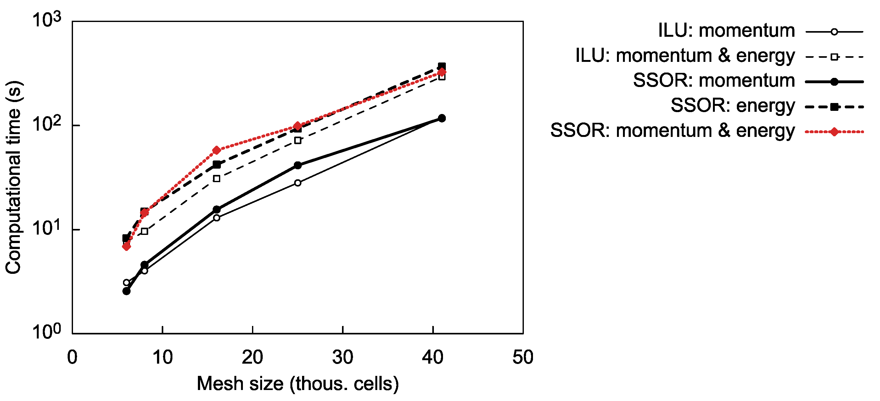
The aim of this study was to establish whether, in the case of simplified CFD models, the SSOR preconditioning technique can be a viable replacement for ILU. From the obtained data, it follows that SSOR should not be used in conjunction with CG to solve the pressure correction equation. When applied to the momentum and/or energy equations, computational times tend to be significantly longer even when the relaxation factors are chosen favorably (for the cases evaluated in this study, the increase was at least ~23% on average). However, because the SSOR preconditioning matrix can always be constructed, the respective techniques could be used in conjunction with ILU as a fallback option. From an engineering point of view, this would mean that ILU would be employed by default, and only in case of numerical issues would the CFD solver try to reach a converged solution using SSOR. Such an approach would capitalize on the efficiency of ILU while maintaining reasonable numerical robustness due to the possibility of falling back to a technique with guaranteed existence of the preconditioning matrix. The resulting models would, ultimately, be much more suitable for implementation in optimization algorithms or for other use cases where large batches of simulations must be carried out without user intervention.

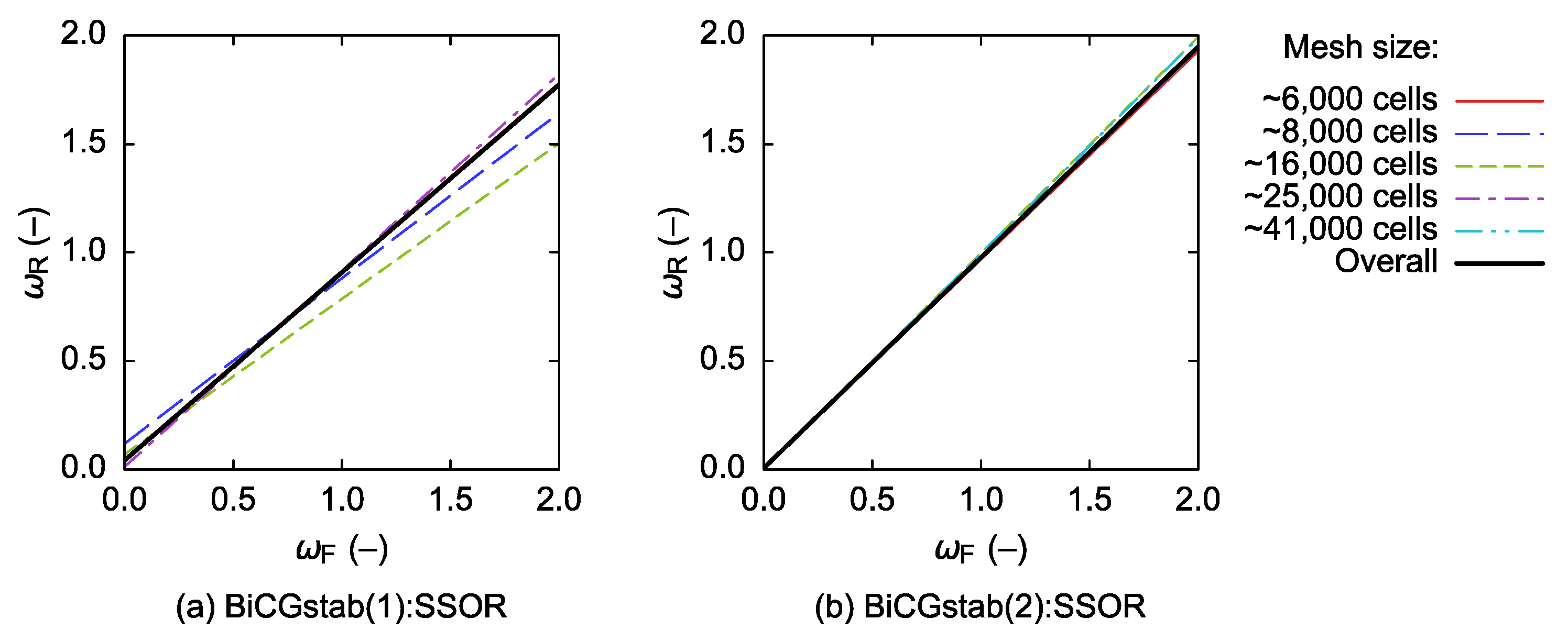
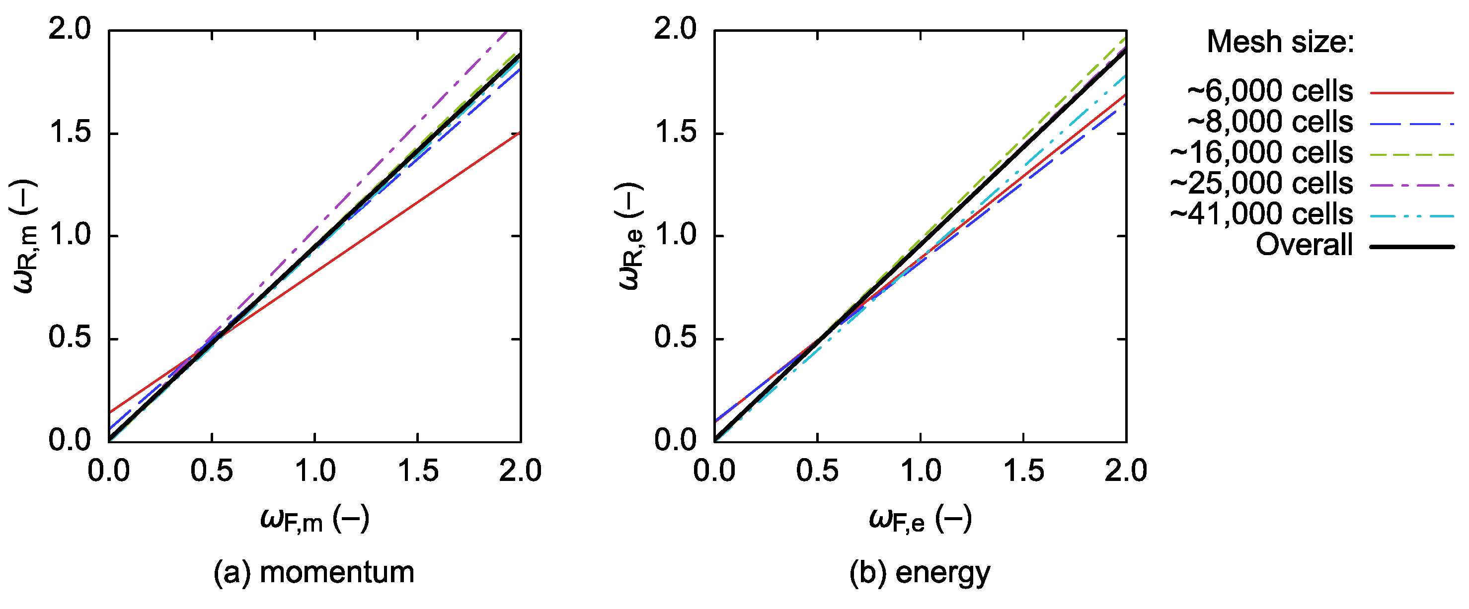
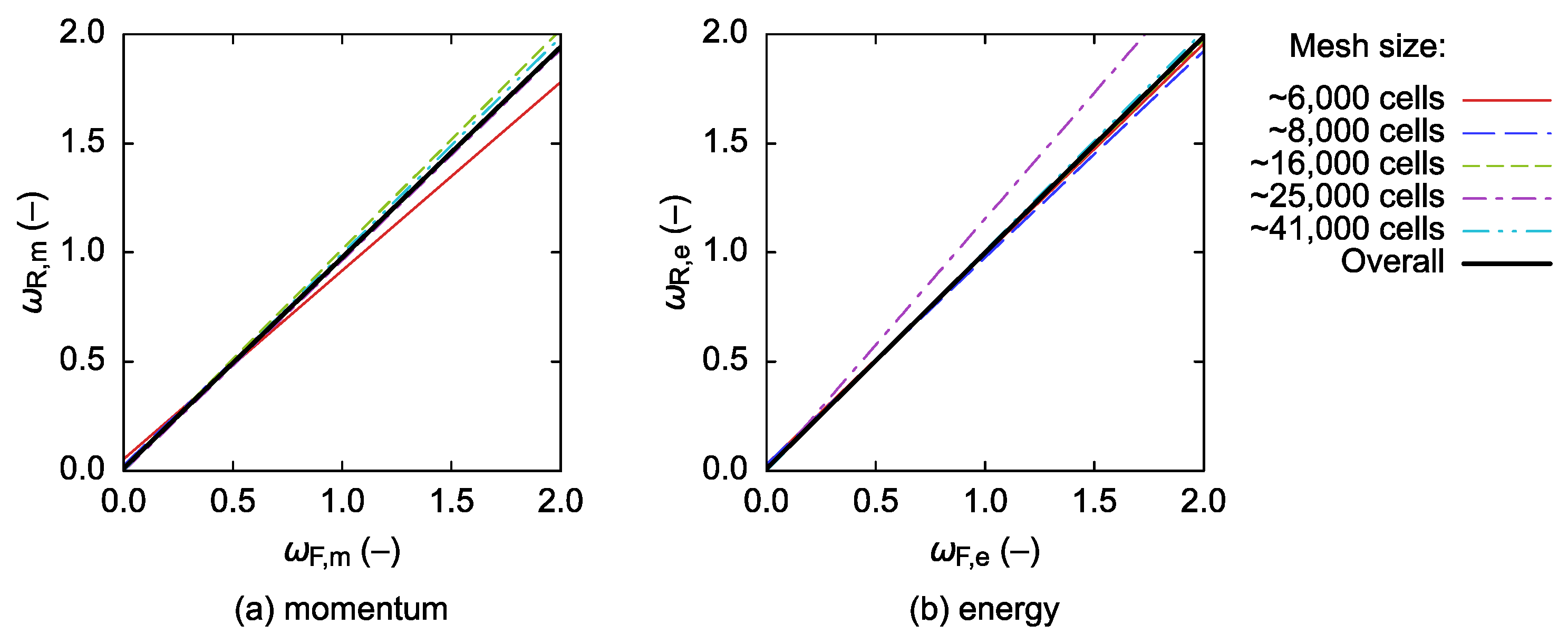
The best-performing combinations of numerical solution methods and SSOR forward and backward relaxation factors differ according to whether energy transport is included in the model or not. In the flow-only scenario, the momentum equations should preferably be solved using BiCGstab(3), with ω_F ≈ 0.9 and ω_R slightly less than ω_F, that is, both SSOR sweeps should be a little underrelaxed. Computational times obtained using other variants of BiCGstab(L) proved to be at least 80% longer. If also the energy transport is included and only the energy equation is preconditioned using SSOR, it is best to solve the momentum equations using BiCGstab(3) and the energy equation using BiCGstab(1). Here, both SSOR sweeps should be slightly overrelaxed, with ω_F ≈ 1.2 and ω_R ≈ 1.1. Similar performance can in some cases be obtained by employing BiCGstab(2) for both types of equations with the energy SSOR sweeps being overrelaxed using ω_F ≈ ω_R ≈ 1.1; however, a much greater solution failure probability can then be expected. If SSOR is utilized for both the momentum and the energy equations, then it is, again, preferable to use the combination of BiCGstab(3) and BiCGstab(1). The respective forward sweeps should be a little overrelaxed (ω_F between ca. 1.1 and 1.3 for the momentum, and up to ca. 1.2 for the energy), while the backward sweeps should feature ω_R slightly lower than ω_F. The best-case computational times obtained with BiCGstab(2) proved to be up to ~67% longer and, therefore, the use of this numerical solution method is discouraged in this scenario.

References

1. Turek, V.; Fialová, F.; Jegla, Z. Efficient flow modelling in equipment containing porous elements. Chem. Eng. Trans. 2016, 52, 487–492. [Google Scholar] [CrossRef]
2. Meijerink, J.A.; van der Vorst, A.H. An iterative solution method for linear systems of which the coefficient matrix is a symmetric M-matrix. Math. Comput. 1977, 31, 148–162. [Google Scholar] [CrossRef]
3. Chapman, A.; Saad, Y.; Wigton, L. High-order ILU preconditioners for CFD problems. Int. J. Numer. Methods Fluids 2000, 33, 767–788. [Google Scholar] [CrossRef]
4. Young, D.M. On the accelerated SSOR method for solving large linear systems. Adv. Math. 1977, 23, 215–271. [Google Scholar] [CrossRef] [Green Version]
5. Birken, P.; Gassner, G.; Haas, M.; Munz, C.-D. Preconditioning for modal discontinuous Galerkin methods for unsteady 3D Navier–Stokes equations. J. Comput. Phys. 2013, 240, 20–35. [Google Scholar] [CrossRef]
6. Bai, Z.-Z. On SSOR-like preconditioners for non-Hermitian positive definite matrices. Numer. Linear Algebra 2016, 23, 37–60. [Google Scholar] [CrossRef]
7. Tan, X.-Y. Shifted SSOR-like preconditioner for non-Hermitian positive definite matrices. Numer. Algorithms 2017, 75, 245–260. [Google Scholar] [CrossRef]
8. Zhang, J.-L. On SSOR-like preconditioner for saddle point problems with dominant skew-Hermitian part. Int. J. Comput. Math. 2019, 96, 782–796. [Google Scholar] [CrossRef]
9. Wang, Z.-Q. On hybrid preconditioning methods for large sparse saddle-point problems. Linear Algebra Appl. 2011, 434, 2353–2366. [Google Scholar] [CrossRef]
10. Chen, J.; Liu, Z.; Cao, N.; Yong, B. Shifted SSOR preconditioning technique for improved electric field integral equations. Microw. Opt. Technol. Lett. 2013, 55, 304–308. [Google Scholar] [CrossRef]
11. Wu, S.-L.; Li, C.-X. A modified SSOR preconditioning strategy for Helmholtz equations. J. Appl. Math. 2012, 2012, 365124. [Google Scholar] [CrossRef]
12. Zhang, L.T.; Cheng, S.H. Modified block symmetric SOR preconditioners for large sparse saddle-point problems. Appl. Mech. Mater. 2013, 241–244, 2583–2586. [Google Scholar] [CrossRef]
13. Huang, Y.-M.; Lu, D.-Y. A preconditioned conjugate gradient method for multiplicative half-quadratic image restoration. Appl. Math. Comput. 2013, 219, 6556–6564. [Google Scholar] [CrossRef]
14. Meng, Z.; Li, F.; Xu, X.; Huang, D.; Zhang, D. Fast inversion of gravity data using the symmetric successive over-relaxation (SSOR) preconditioned conjugate gradient algorithm. Explor. Geophys. 2017, 48, 294–304. [Google Scholar] [CrossRef]
15. Helfenstein, R.; Koko, J. Parallel preconditioned conjugate gradient algorithm on GPU. J. Comput. Appl. Math. 2012, 236, 3584–3590. [Google Scholar] [CrossRef] [Green Version]
16. Meyer, K. Technical note: A successive over-relaxation preconditioner to solve mixed model equations for genetic evaluation. J. Anim. Sci. 2016, 94, 4530–4535. [Google Scholar] [CrossRef] [PubMed]
17. Sanjuan, G.; Margalef, T.; Cortés, A. Accelerating preconditioned conjugate gradient solver in wind field calculation. In Proceedings of the 2016 International Conference on High Performance Computing & Simulation (HPCS), Innsbruck, Austria, 18–22 July 2016; Smari, W.W., Ed.; IEEE: New York, NY, USA, 2016; pp. 294–301. [Google Scholar] [CrossRef]
18. Duff, I.S.; Meurant, G.A. The effect of ordering on preconditioned conjugate gradients. BIT Numer. Math. 1989, 29, 635–657. [Google Scholar] [CrossRef]
19. DeLong, M.A.; Ortega, J.M. SOR as a preconditioner. Appl. Numer. Math. 1995, 18, 431–440. [Google Scholar] [CrossRef]
20. Chen, Y.; Zhao, Y.; Zhao, W.; Zhao, L. A comparative study of preconditioners for GPU-accelerated conjugate gradient solver. In Proceedings of the 2013 IEEE 10th International Conference on High Performance Computing and Communications & 2013 IEEE International Conference on Embedded and Ubiquitous Computing, Zhangjiajie, China, 13–15 November 2013; IEEE: New York, NY, USA, 2013; pp. 628–635. [Google Scholar] [CrossRef]
21. Li, J.; Zhang, N.-M. A triple-parameter modified SSOR method for solving singular saddle point problems. BIT Numer. Math. 2016, 56, 501–521. [Google Scholar] [CrossRef]
22. Pan, C. On generalized SSOR-like iteration method for saddle point problems. WSEAS Trans. Math. 2017, 16, 239–247. [Google Scholar]
23. Liang, Z.-Z.; Zhang, G.-F. Modified unsymmetric SOR method for saddle-point problems. Appl. Math. Comput. 2014, 234, 584–598. [Google Scholar] [CrossRef]
24. Wang, H.-D.; Huang, Z.-D. On a new SSOR-like method with four parameters for the augmented systems. East Asian J. Appl. Math. 2017, 7, 82–100. [Google Scholar] [CrossRef]
25. Louka, M.A.; Missirlis, N.M. A comparison of the extrapolated successive overrelaxation and the preconditioned simultaneous displacement methods for augmented linear systems. Numer. Math. 2015, 131, 517–540. [Google Scholar] [CrossRef]
26. Najafi, H.S.; Edalatpanah, S.A. On the modified symmetric successive over-relaxation method for augmented systems. Comp. Appl. Math. 2015, 34, 607–617. [Google Scholar] [CrossRef]
27. Darvishi, M.T.; Hessari, P. A modified symmetric successive overrelaxation method for augmented systems. Comput. Math. Appl. 2011, 61, 3128–3135. [Google Scholar] [CrossRef] [Green Version]
28. Salkuyeh, D.K.; Shamsi, S.; Sadeghi, A. An improved symmetric SOR iterative method for augmented systems. Tamkang J. Math. 2012, 43, 479–490. [Google Scholar] [CrossRef]
29. Huang, Z.-G.; Wang, L.-G.; Xu, Z.; Cui, J.-J. Preconditioned accelerated generalized successive overrelaxation method for solving complex symmetric linear systems. Comput. Math. Appl. 2019, 77, 1902–1916. [Google Scholar] [CrossRef]
30. Edalatpour, V.; Hezari, D.; Salkuyeh, D.K. Accelerated generalized SOR method for a class of complex systems of linear equations. Math. Commun. 2015, 20, 37–52. [Google Scholar]
31. Hezari, D.; Edalatpour, V.; Salkuyeh, D.K. Preconditioned GSOR iterative method for a class of complex symmetric system of linear equations. Numer. Linear Algebra Appl. 2015, 22, 761–776. [Google Scholar] [CrossRef] [Green Version]
32. Salkuyeh, D.K.; Hezari, D.; Edalatpour, V. Generalized successive overrelaxation iterative method for a class of complex symmetric linear system of equations. Int. J. Comput. Math. 2015, 92, 802–815. [Google Scholar] [CrossRef]
33. Pu, Z.-N.; Wang, X.-Z. Block preconditioned SSOR methods for H-matrices linear systems. J. Appl. Math. 2013, 2013, 213659. [Google Scholar] [CrossRef]
34. Kushida, N. Condition number estimation of preconditioned matrices. PLoS ONE 2015, 10, e0122331. [Google Scholar] [CrossRef] [PubMed]
35. Zhang, C.; Miao, G.; Zhu, Y. Convergence on successive over-relaxed iterative methods for non-Hermitian positive definite linear systems. J. Inequal. Appl. 2016, 2016, 156. [Google Scholar] [CrossRef]
36. Wang, H.-D.; Huang, Z.-D. On convergence and semi-convergence of SSOR-like methods for augmented linear systems. Appl. Math. Comput. 2018, 326, 87–104. [Google Scholar] [CrossRef]
37. Liang, Z.-Z.; Zhang, G.-F. On SSOR iteration method for a class of block two-by-two linear systems. Numer. Algorithms 2016, 71, 655–671. [Google Scholar] [CrossRef]
38. Zhou, L.; Zhang, N. Semi-convergence analysis of GMSSOR methods for singular saddle point problems. Comput. Math. Appl. 2014, 68, 596–605. [Google Scholar] [CrossRef]
39. Cao, G.; Huang, Y.; Song, Y. Convergence of parallel block SSOR multisplitting method for block H-matrix. Calcolo 2013, 50, 239–253. [Google Scholar] [CrossRef]
40. Yang, S.; Gobbert, M.K. The optimal relaxation parameter for the SOR method applied to the Poisson equation in any space dimensions. Appl. Math. Lett. 2009, 22, 325–331. [Google Scholar] [CrossRef] [Green Version]
41. Barrett, R.; Berry, M.W.; Chan, T.F.; Demmel, J.; Donato, J.; Dongarra, J.; Eijkhout, V.; Pozo, R.; Romine, C.; Van der Vorst, H. Templates for the Solution of Linear Systems: Building Blocks for Iterative Methods, 2nd ed.; Society for Industrial and Applied Mathematics (SIAM): Philadelphia, PA, USA, 1994; pp. 35–49. [Google Scholar]
42. Turek, V. On improving computational efficiency of simplified fluid flow models. Chem. Eng. Trans. 2018, 70, 1447–1452. [Google Scholar] [CrossRef]
43. Van Doormaal, J.P.; Raithby, G.D. Enhancement of the SIMPLE method for predicting incompressible fluid flows. Numer. Heat Transf. 1984, 7, 147–163. [Google Scholar] [CrossRef]
44. Patankar, S.V. A calculation procedure for two-dimensional elliptic situations. Numer. Heat Transf. 1981, 4, 409–425. [Google Scholar] [CrossRef]
45. Hestenes, M.R.; Stiefel, E. Methods of conjugate gradients for solving linear systems. J. Res. Natl. Bur. Stand. 1952, 49, 409–436. [Google Scholar] [CrossRef]
46. Sleijpen, G.L.; Fokkema, D.R. BiCGstab(l) for linear equations involving unsymmetric matrices with complex spectrum. Electron. Trans. Numer. Anal. 1993, 1, 11–32. [Google Scholar]
Figure 1. Sample simplified (cuboid cell-only) meshes generated automatically by the benchmarking software using the growth factor of 1.15; clockwise from top left: (a) layout of the “Z”-arranged flow system 1 from Table 1; (b) the corresponding finer mesh (~25,000 cells, groups of red cells in the top view denote locations of tube cross-sections); (c) top view of the finer mesh of the distribution header from flow system 2 (inlet region being on the left); other parts of this mesh, as well as the remaining meshes, were generated analogously.
Energies 12 02438 g001
Figure 2. Mean computational times for three different meshes and various combinations of ωF and ωR, the pressure correction equation was solved using CG:SSOR and the momentum equations using BiCGstab(3):ILU; diagonal crosses indicate failing combinations of ωF and ωR. Please note that the colorbars have been adjusted so that the best (i.e., the most relevant) combinations of ωF, ωR are easily identifiable. Further, due to the necessary colorbar ranges, the respective lower limits have been set to zero even though the data start at higher values.
Energies 12 02438 g002
Figure 3. Mean computational times for the smallest mesh and the cases when the pressure correction equation was solved using CG:ILU and the momentum equations using BiCGstab(3):SSOR, BiCGstab(2):SSOR, and BiCGstab(1):SSOR; diagonal crosses indicate failing combinations of ωF and ωR. Please note that the colorbars have been adjusted so that the best (i.e., the most relevant) combinations of ωF, ωR are easily identifiable.
Energies 12 02438 g003
Figure 4. Mean computational times for the neighborhoods of pivot points corresponding to the smallest mesh; the pressure correction equation was solved using CG:ILU and the momentum equations using BiCGstab(3):SSOR; please note that, for the sake of clarity, the time ranges have been severely limited in both plots. Again, the colorbars have been adjusted so that the best (i.e., the most relevant) combinations of ωF, ωR are easily identifiable.
Energies 12 02438 g004
Figure 5. Relaxation factor trends for the solution of momentum equations using BiCGstab(3):SSOR; the overall trend was obtained using the merged data set and identical weights.
Energies 12 02438 g005
Figure 6. Mean computational times for three different meshes and various combinations of ωF and ωR, CG:ILU was used to solve the pressure correction equation, BiCGstab(3):ILU was used for the momentum equations, and BiCGstab(1):SSOR was used for the energy equation; diagonal crosses indicate failing combinations of ωF and ωR. Please note that the colorbars have been adjusted so that the best (i.e., the most relevant) combinations of ωF, ωR are easily identifiable.
Energies 12 02438 g006
Figure 7. Mean computational times corresponding to the meshes from Figure 6 and the cases when the momentum equations were solved using BiCGstab(2):ILU, and the energy equation was solved using BiCGstab(2):SSOR; diagonal crosses indicate failing combinations of ωF and ωR. Please note that the colorbars have been adjusted so that the best (i.e., the most relevant) combinations of ωF, ωR are easily identifiable.
Energies 12 02438 g007
Figure 8. Relaxation factor trends for the two discussed setups using either BiCGstab(1):SSOR or BiCGstab(2):SSOR to solve the energy equation; the overall trends were obtained using the merged data sets and identical weights.
Energies 12 02438 g008
Figure 9. Two-dimensional plots of mean computational times obtained for the smallest “Z”-arranged mesh with (a) the energy relaxation factor tuple fixed to (ωF, ωR) = (1.2, 0.7) and (b) the momentum relaxation factor tuple fixed to (ωF, ωR) = (1.3, 1.1); BiCGstab(3):SSOR was used to solve the momentum equations and BiCGstab(1):SSOR the energy equation. Please note that the colorbars have been adjusted so that the best (i.e., the most relevant) combinations of ωF, ωR are easily identifiable.
Energies 12 02438 g009
Figure 10. Two-dimensional plots of mean computational times obtained for the smallest “Z”-arranged mesh with (a) the energy relaxation factor tuple fixed to (ωF, ωR) = (0.9, 1.2) and (b) the momentum relaxation factor tuple fixed to (ωF, ωR) = (1.0, 0.9); BiCGstab(2):SSOR was used to solve both the momentum equations and the energy equation; diagonal crosses indicate failing combinations of ωF and ωR. Please note that the colorbars have been adjusted so that the best (i.e., the most relevant) combinations of ωF, ωR are easily identifiable.
Energies 12 02438 g010
Figure 11. Relaxation factor trends for (a) momentum and (b) energy obtained with BiCGstab(3):SSOR and BiCGstab(1):SSOR as the solution methods for the momentum equations and the energy equation, respectively; the overall trends were obtained using the merged data sets and identical weights.
Energies 12 02438 g011
Figure 12. Relaxation factor trends for (a) momentum and (b) energy obtained with BiCGstab(2):SSOR as the solution method for both the momentum equations and the energy equation; the overall trends were obtained using the merged data sets and identical weights.
Energies 12 02438 g012
Figure 13. Comparison of the mean computational times obtained when solely the ILU preconditioning technique was used, and the overall best-case mean computational times reached with the momentum equations and/or the energy equation being preconditioned with SSOR.
Energies 12 02438 g013