Deep Learning Neural Networks Trained with MODIS Satellite-Derived Predictors for Long-Term Global Solar Radiation Prediction

Abstract

Solar energy predictive models designed to emulate the long-term (e.g., monthly) global solar radiation (GSR) trained with satellite-derived predictors can be employed as decision tenets in the exploration, installation and management of solar energy production systems in remote and inaccessible solar-powered sites. In spite of a plethora of models designed for GSR prediction, deep learning, representing a state-of-the-art intelligent tool, remains an attractive approach for renewable energy exploration, monitoring and forecasting. In this paper, algorithms based on deep belief networks and deep neural networks are designed to predict long-term GSR. Deep learning algorithms trained with publicly-accessible Moderate Resolution Imaging Spectroradiometer (MODIS) satellite data are tested in Australia’s solar cities to predict the monthly GSR: single hidden layer and ensemble models. The monthly-scale MODIS-derived predictors (2003–2018) are adopted, with 15 diverse feature selection approaches including a Gaussian Emulation Machine for sensitivity analysis used to select optimal MODIS-predictor variables to simulate GSR against ground-truth values. Several statistical score metrics are adopted to comprehensively verify surface GSR simulations to ascertain the practicality of deep belief and deep neural networks. In the testing phase, deep learning models generate significantly lower absolute percentage bias (≤3%) and high Kling–Gupta efficiency (≥97.5%) values compared to the single hidden layer and ensemble model. This study ascertains that the optimal MODIS input variables employed in GSR prediction for solar energy applications can be relatively different for diverse sites, advocating a need for feature selection prior to the modelling of GSR. The proposed deep learning approach can be adopted to identify solar energy potential proactively in locations where it is impossible to install an environmental monitoring data acquisition instrument. Hence, MODIS and other related satellite-derived predictors can be incorporated for solar energy prediction as a strategy for long-term renewable energy exploration.

1. Introduction and Background

Due to the decreasing trends of feed-in tariffs (a premium rate paid for electricity fed back into the electricity grid from a designated renewable electricity generation source) for solar-generated electricity in many countries (including Australia), there has been an accelerated interest and need for versatile energy management systems (EMS) for end-users to increase the generation of electricity and the capacity for power transmission from various regions, both remote and metropolitan, to meet the rising consumer energy demands [1]. EMS are able to monitor, control and optimize the transmission and use of solar and conventional energies [2]. However, the prediction error on the power output from a solar power system can cause a negative effect on the system profitability. Considering this, an accurate predictive tool for solar can help reduce the uncertainty of power generation (solar photovoltaic), as well as to increase the conversion efficiency (solar thermal) in the future. Such tools can be used to explore and evaluate the sustainability of long-term solar-powered energy installations in all regions, irrespective of their location.

The magnitude of power generated by a solar photovoltaic (PV) system and conversion efficiency (solar air heater, solar water heater, solar concentrator) is largely a function of the global solar radiation (GSR) [3]. However, stochastic components of solar energy variability depend on the cloud coverage characteristics, as well as factors including the aerosol, dust particles, smoke and airborne pollutants that are largely difficult to measure on an ongoing basis and, therefore, must be derived from remotely-sensed data products. In addition to this, the intermittency and randomness in atmospheric variables and a lack of data for remote or regional sites make the prediction of long-term availability of GSR to support a future solar PV, as well as a solar thermal system quite challenging. Although GSR is one of the most commonly-monitored meteorological variables, measurement stations remain sparse, particularly in the Southern Hemisphere [4]. Even if a measurement station has been set up, the measured data can be unreliable and questionable, due to a lack of regular maintenance and issues with calibration of the instruments in a regional or remote location [5]. To surmount these issues, the opportunity to adopt satellite-derived predictors to estimate long-term GSR presents an alternative and viable avenue for future exploration of solar energy.

To explore solar energy potentials, many techniques have been developed to predict GSR, which can be largely categorized as follows: (I) empirical models with simple mathematical equations: linear, quadratic and polynomial equations to emulate the links between GSR and its related meteorological variables; (II) remote sensing retrieval that is based on images from satellites used to predict GSR [6]; (III) soft computing or data-driven models that apply artificial intelligence techniques to model the erratic behaviour of GSR received on the Earth’s surface. The requirement for any predictive model for solar applications is that it must be an appropriately representative model developed, calibrated and validated to extract intrinsic features related to GSR prediction.

Data-driven models are becoming increasingly promising tools for electrical power [7,8] and solar radiation prediction [9,10,11,12,13,14]. Single hidden layer (SHL) neural networks, using the artificial neural network (ANN) as a black-box tool, have been designed for both short-term [15] and long-term prediction of GSR [13,16]. A recent study in Australia designed an ANN model at four locations using the European Centre for Medium Range Weather Forecasting (ECMWF) reanalysis data as an input [10]. In spite of the acceptable performance in this study, inputs were selected from a limited set of meteorological variables from weather stations (e.g., latitude, rainfall, sunshine duration, humidity, temperature) and, therefore, did not consider additional predictors, such as those available in satellite data repositories that could possibly influence GSR.

To address the potential problems associated with the inadequacy of data, the opportunity to use satellite products from the National Aeronautics and Space Administration (NASA), Goddard Online Interactive Visualization and Analysis Infrastructure (GIOVANNI) repository is an alternative avenue to generate GSR forecasts, particularly feeding the model with important variables such as land surface temperature, cloud-free days, aerosol optical depth and cloud temperature that are highly likely to moderate the amount of solar radiation received at the Earth’s surface. In fact, recent studies have utilized land surface temperature with other satellite-derived variables to model long-term GSR in regional Queensland and over the Australian sub-continent [9,13], although none have used a sophisticated method (e.g., deep learning algorithms).

Recently, to address potential limitations of ANNs, particularly arising from the algorithm being a single hidden layer neuronal system, a number of newer neural network techniques such as deep learning (DL) have also been implemented [17] and shown to generate a superior accuracy compared to a single hidden layer model. Deep learning is designed to use a neural network structure similar to the ANN to represent inputs and target data. These models use multiple feature extraction layers and learn the complex relationships within the data more efficiently. These DL methods have been widely implemented in medical imaging, speech recognition and natural language processing, autonomous driving and computer vision. However, there have been only a few prior studies that have employed a DL model for GSR prediction, especially using satellite-derived predictor datasets.

To address the limitations of single hidden layer neuronal models, this paper adopts the deep neural network (DNN) and deep belief network (DBN), the two fundamental categories of DL algorithms, coupled with satellite-derived data to predict long-term GSR, where monthly averaged daily values are modelled for solar cities in Australia. These solar cities have previously been established as potential future sites for solar energy projects that have a low cloud cover and limited aerosol concentrations and are thus well suited for solar energy. To provide a sound context for developing DNN and DBN models to predict the GSR, the merits of DL models include the capability to extract much deeper and naturally inherent data features within a predictor-target matrix, mainly to provide more accurate predictions [18]. For example, a DNN approach is able to boost the predictive power of the ANN model by deepening and replicating its hidden layers and also leveraging its internal structures to model the GSR accurately. Moreover, a DBN model [19] is able to avoid the problem of overfitting and also avoiding the learning mode being halted when a local optima emerges in a feature space. The merits of deep learning models can, therefore, help address the unavoidable drawbacks of conventional approaches, e.g., an ANN model [20].

Many studies are currently using deep learning for time series forecasts [21,22,23,24]. Some results reveal a DBN model’s superiority over a linear autoregressive and a conventional back-propagation neural network (i.e., ANN) model. Furthermore, literature on GSR prediction problems using deep learning approaches has rather been limited to short-term forecast horizons (i.e., minutes and hours), and these studies have used deep learning based on long short term memory network or convolutional neural networks. However, a longer forecast horizon (i.e., weekly or monthly model) can be useful for exploring the long-term prospects of solar energy [25], leading to better policy, implementation of new solar powered sites and expansion of solar energy systems in remote and regional locations where solar radiation may be in abundance [9,10,13].

A literature review, particularly the related review articles [26,27,28], shows that the current literature is relatively scarce, and even non-existent, in terms of prior studies conducted to predict monthly GSR using deep learning approaches. From a practical point of view, the future planning for an electricity grid certainly requires the prediction of solar radiation a few months ahead of time [29]; therefore, a monthly predictive model is particularly desirable. That model can be useful for agricultural crop growth [30], production of algal-derived biofuels [31], and key decisions made for many applications, where the estimation of long-term solar radiation may be required.

The aims of this study are as follows: (1) to design and implement a deep learning (DL) approach using deep belief network (DBN) and deep neural network (DNN) algorithms and to evaluate its relative success in estimating the long-term daily average monthly GSR using remotely-sensed MODIS-derived products as the DL model’s input variables. Here, we consider the application study site as Australia’s solar cities, namely: Blacktown [33.77°S, 150.90°E], Adelaide [34.92°S, 138.59°E], Townsville [19.25°S, 146.81°E] and Central Victoria [36.74°S, 144.28°E], all four of which are situated in the dry sub-tropic region and are relatively enriched with solar exposure. The next aims of the study are: (2) to apply wrapper and filter-based feature selection techniques on the MODIS satellite data in order to select the optimum predictor variables for these prescribed DL models; (3) to adopt the Gaussian Emulation Machine approach to perform a sensitivity analysis of MODIS variables to deduce their relative influence on GSR prediction; (4) to benchmark the deep learning models (i.e., DBN and DNN) with a multitude of competing data-driven approaches, namely: single hidden layer (ANN), and ensemble models (random forest regression (RF), extreme gradient boosting regression (XGBR), Gradient Boosting Machine (GBM), and decision tree (DT).

By testing the developed models over Australia’s solar cities, this paper aims to provide valuable contributions to exploring the utility of a deep learning approach of improving other previous studies (e.g., [10,11,12,13]) where single hidden layer neuronal systems have been used. The novelty lies in the incorporation of MODIS-derived predictors to foster new insights for estimating long-term solar energy for any region that does not have atmospheric monitoring systems. More importantly, it can rely on remote sensing data for GSR prediction. These models can promote solar energy in remote or regional areas where satellites can be employed for long-term evaluation.

2. Theoretical Background

In this section, only the deep learning models are explained in detail; the theoretical explanation of the ANN [32], RF [33], GBM [34], XGBR [35] and DT [36,37] is all elucidated elsewhere since they are well-known methodologies.

2.1. Objective Model: Deep Learning Approach

Deep learning (DL) is a subfield of data-driven models where the algorithm itself learns the internal representation from raw data to perform a regression or a classification process. This is in contrast to classical methods that require carefully-engineered input features based on domain expertise. The DL algorithm can be classified with artificial neural networks because of its multi-layer structure formed by input and output neurons. The multi-layer network as a class of data-driven methods is built by attaching multiple layers to form a unique machine. The DL methodology aims to sequence independent machines, in which the output of one layer is the input of the next layer.

In this paper, we adopt DL as it has recently been used to predict renewable energy sources. For example, the work in [38] used deep belief network (DBN) to predict wind power, whereas [39] applied stacked auto encoders to predict short-term wind speed. Hence, two fundamental forms of DL, based on DNN and DBN, are used to predict GSR by employing MODIS-derived predictor variables.

2.1.1. Deep Belief Network

Deep belief network (DBN) is a generative model with a stacked restricted Boltzmann machine (RBM) and a sigmoid belief network. A typical DBN algorithm flowchart is shown in Figure 1a. The deep belief network plays an important role in modelling time series data [23] and has been adopted in energy studies, for example wind speed prediction [40,41].

The proposed DBN GSR prediction model is comprised of two RBMs and one MLP (Figure 1b). The RBM is symmetrical bipartite with two layers (visible and hidden layer). The visible units $v=\{v_1,v_2,\cdots ,v_m\}$ and the hidden units $h=\{h_1,h_2,\cdots ,h_n\}$ are connected by a symmetrical weight matrix W, as well as bias weights (offsets) $a=\left\{a_i\right|i=1,2,\cdots ,m\}$ for the visible units and $b=\left\{b_j\right|j=1,2,\cdots ,n\}$ for the hidden units. RBM is an energy model, and the energy function of the visible layer and hidden layer is defined as below [42]:

$$\begin{array}{l}E(v,h;\theta )=-{\displaystyle {\displaystyle \sum }_{i=1}^{n_v}}{a}_i{v}_i-{\displaystyle {\displaystyle \sum }_{j=1}^{n_h}}{b}_j{h}_j-{\displaystyle {\displaystyle \sum }_{i=1}^{n_v}}{\displaystyle {\displaystyle \sum }_{j=1}^{n_h}}{h}_j{W}_{j,i}{v}_i\\ \mathrm{where}\\ v_i=\mathrm{number}\mathrm{of}\mathrm{neurons}\mathrm{in}\mathrm{the}\mathrm{visible}\mathrm{layer};\\ a_i=\mathrm{is}\mathrm{the}\mathrm{bias}\mathrm{of}\mathrm{node}i;\\ b_j=\mathrm{is}\mathrm{the}\mathrm{bias}\mathrm{of}\mathrm{node}j;\\ h_j=\mathrm{is}\mathrm{the}\mathrm{number}\mathrm{of}\mathrm{Boolean}\mathrm{hidden}\mathrm{neurons}\\ \mathrm{within}\mathrm{the}\mathrm{hidden}\mathrm{layer};\\ W_{j,i}=\mathrm{is}\mathrm{the}\mathrm{weight}\mathrm{matrices}\mathrm{between}\mathrm{the}\\ \mathrm{visible}\mathrm{layer}\mathrm{and}\mathrm{hidden}\mathrm{layer};\\ \theta =\mathrm{is}\mathrm{a}\mathrm{model}\mathrm{parameter},\theta =\{w,a,b\};\end{array}$$

(1)

In order to minimize the energy function, i.e., Equation (1), the model parameters $\theta =\left\{W,a,b\right\}$ of RBM need to be updated by the contrastive divergence algorithm proposed by Hinton [43], and the update rule can be derived by Equation (2) [44].

$$\begin{array}{l}\mathsf{\Delta }\mathbf{W}=\epsilon ({\mathrm{vh}}^T-{\mathbf{v}}^{\prime }{\mathbf{h}}^{\prime T})\\ \mathsf{\Delta }\mathbf{a}=\epsilon (\mathrm{v}-{\mathrm{v}}^{\prime })\\ \mathsf{\Delta }\mathbf{b}=\epsilon (\mathbf{h}-{\mathbf{h}}^{\prime })\end{array}$$

(2)

where ε is the learning rate and V′ and h’ are the reconstruction of v and h by Gibbs sampling [45], respectively. Once the first RBM is trained, its hidden layer becomes the visible layer of the next RBM, and the new RBM is trained with the procedure above. Then, a supervised learner MLP is added to the top of the network for time series forecasting. Finally, the parameters of the whole network are fine-tuned by the back-propagation algorithm.

2.1.2. Deep Neural Network

Deep neural networks (DNNs) are complex, yet fully-connected ANNs composed of more than one hidden layer (Figure 1c), where each successive layer uses the outputs from the previous layer. Although different architectures are available, a common DL has a feed-forward network, with a back-propagation algorithm, for the learning and optimization. Although DNNs exhibit superior performance, overfitting is the major issue, which can be decreased by applying a regularization technique such as a weight penalty, early stopping or dropout during training. The input layer of the DNN implemented in this study is selected using the feature selection procedure (Section 3) where one neuron in the output layer is used to generate the predicted GSR. The mathematical form of the neural network forward propagation model is described below [46]:

$$\begin{array}{l}{a}^l{}_i=f\left({\displaystyle {\displaystyle \sum }_{j=1}^{N^{l-1}}}{W}_{ij}{}^l{a}_j{}^{l-1}+b_i{}^l\right)\\ \mathrm{where}\\ a^l{}_i=\mathrm{output}\mathrm{value}\mathrm{from}\mathrm{the}{i}^{th}\mathrm{neurons}\mathrm{in}\mathrm{the}{l}^{th}\mathrm{layer}\mathrm{neural}\mathrm{network}.\\ a_j{}^{l-1}=\mathrm{output}\mathrm{value}\mathrm{from}\mathrm{the}{i}^{th}\mathrm{neurons}\mathrm{in}\mathrm{the}{(l-1)}^{th}\mathrm{layer}\mathrm{neural}\mathrm{network}\\ W_{ij}{}^l=\mathrm{the}\mathrm{weight}\mathrm{from}\mathrm{the}{j}^{th}\mathrm{neurons}\mathrm{in}\mathrm{the}{(l-1)}^{th}\mathrm{layer}\mathrm{to}\mathrm{the}{i}^{th}\mathrm{neurons}\mathrm{in}\mathrm{the}{l}^{th}\mathrm{layer}.\\ b_i{}^l=\mathrm{bias}\mathrm{term}\mathrm{from}\mathrm{the}{i}^{th}\mathrm{neurons}\mathrm{in}\mathrm{the}{l}^{th}\mathrm{layer}\mathrm{neural}\mathrm{network}.\\ N^{l-1}=\mathrm{number}\mathrm{of}\mathrm{neurons}\mathrm{in}\mathrm{the}{(l-1)}^{th}\mathrm{layer}.\\ f(•)=\mathrm{is}\mathrm{the}\mathrm{activation}\mathrm{function}\mathrm{of}\mathrm{the}\mathrm{neurons}.?\end{array}$$

(3)

Among the many types of neural network activation functions, a popular one includes the sigmoid function, ReLU (rectified linear unit), softplus and hyperbolic tangent (tanh) [47] functions, described as follows:

$$\begin{array}{l}f\left(x\right)=\frac{1}{1+e^{-x}}=\mathit{sigmoid}\mathit{function}(\sigma )\\ f\left(x\right)=\frac{e^{2x}-1}{e^{2x}+1}=\mathit{tanhfunction}\\ f\left(x\right)=\mathit{ln}\left(e^x+1\right)-\mathit{ln}2=\mathit{softplus}\mathit{function}\\ f\left(x\right)=\mathit{max}\left(0,x\right)=\mathit{Re}LU\mathit{function}\\ wherexistheinputtoaneuron\end{array}$$

(4)

The mean squared error of training sets can be described by [32]:

$$\begin{array}{l}mse=\frac{1}{m}{\displaystyle {\displaystyle \sum }_{t=1}^m}{\left(o_t-y_t\right)}^2=T\left(w\right)\\ \mathrm{where}\\ mse=\mathrm{mean}\mathrm{squared}\mathrm{error}\mathrm{between}\mathrm{the}\mathrm{predicted}\mathrm{and}\mathrm{true}\mathrm{values}\mathrm{of}\mathrm{the}\mathrm{data}\mathrm{sets}.\\ o_t=t^{th}\mathrm{sample}’\mathrm{s}\mathrm{predicted}\mathrm{value}\mathrm{of}GSR.\\ y_t=t^{th}\mathrm{sample}’\mathrm{s}\mathrm{actual}\mathrm{value}\mathrm{of}GSR\\ w=\mathrm{vector}\mathrm{that}\mathrm{contains}\mathrm{the}\mathrm{weights}\mathrm{and}\mathrm{bias}\mathrm{terms}\mathrm{between}\mathrm{the}\mathrm{neurons}\mathrm{in}\mathrm{each}\mathrm{layer}.\\ m=\mathrm{number}\mathrm{of}\mathrm{the}\mathrm{datasets}.\end{array}$$

(5)

This paper uses the adaptive moment estimation (Adam) [48], root mean squared prop (RMSProp) [49], adaptive gradient (AdaGrad) [50], Nesterov-accelerated adaptive moment estimation (Nadam) [51], the variant of Adam based on the infinity norm (Adamax) [48] and the adaptive delta (AdaDelta) [52] algorithm to avoid the model from falling into a local optimal solution. These algorithms applied updated weights to achieve high efficiency and fast convergence. More details regarding the learning algorithm are found in other works [53].

3. Data, Importance and Context of the Study

This study employs monthly averaged daily GSR records to develop a prediction model using DBN and DNN for four solar cities of Australia: Blacktown [33.77°S, 150.90°E], Adelaide [34.92°S, 138.59°E], Townsville [19.25°S, 146.81°E] and Central Victoria [36.74°S, 144.28°E]. Although the potential for use of solar energy in these regions remains high, deep learning-based models for GSR are not easily available. Furthermore, in most states in Australia, the electricity is provided through power plants located in the central and southern areas, and because of this, there are huge transmission and distribution costs and losses [54]. Hence, there is a potential to harness locally available solar energy, particularly in remote sites where solar forecast models are actively being tested [9,10,11,12,13], although the studies are using simplistic models rather than deep learning approaches.

Other than focusing on solar city sites with abundant solar radiation, this study purposely adopts MODIS satellite variables to model GSR since historical data related to the target variable (GSR) play a key role in helping evaluate solar energy availability. Remote sensing data have already been identified as a practical predictor for solar problems [55], so in this view, the coupling of a deep learning model with satellite-derived products is a major improvement over the use of station-based data mainly because the acquisition of satellite imagery can be feasible for inaccessible sites with no measurement infrastructure as long as a footprint is identified. For long-term forecast horizons (e.g., monthly), satellite data remain abundant for a diverse range of spatial and temporal resolutions and, recently, have been adopted in global solar radiation prediction problems [9,13]. Although recent studies have considered solar radiation models trained with MODIS datasets, these were limited to cloud-free predictor variables and land surface temperature. Considering this, significant MODIS data have not been used in previous studies [56], although a recent study [12] has estimated solar radiation using MODIS-derived predictors without a deep learning model.

3.1. MODIS Satellite-Derived Predictor Data

To design a deep learning model for GSR prediction over long time horizons, monthly predictor data have been extracted from 1 March 2000–2018 from NASA’s Goddard Online Interactive Visualization and Analysis Infrastructure (GIOVANNI) repository.

Table 1. Description of Moderate Resolution Imaging Spectroradiometer (MODIS) satellite-derived predictors, with the relevant notation adopted in this study to predict monthly averaged daily solar radiation (GSR) in Australia’s solar cities (data source: Goddard Online Interactive Visualization and Analysis Infrastructure (GIOVANNI) NASA Repository).

Data Source	MODIS-Derived Variable	Notation	Units
GIOVANNI (MODIS Level 3 Atmosphere Products: MOD08_M3)	Aerosol Optical Depth (550) Dark Target Deep Blue Combined	aoddtdbc	none
	Aerosol Optical Depth Land Ocean	aodlc	none
	Aerosol Scattering Angle	asa	none
	Atmospheric Water Vapour Medium	awvm	cm
	Atmospheric Water Vapour High	awvh	cm
	Atmospheric Water Vapour Low	awvl	cm
	Cloud Effective Radius Ice	cefri	μm
	Cloud Effective Radius Liquid	cerl	μm
	Cloud Fraction	cf	none
	Cloud Fraction Day	cfd	none
	Cloud Fraction Night	cfn	none
	Cloud Optical Thickness Combined	cotc	none
	Cloud Optical Thickness Ice	coti	none
	Cloud Optical Thickness Liquid	cotl	none
	Cirrus Reflectance	cr	none
	Cloud Top Pressure Night	ctp	hPa
	Cloud Top Pressure	ctpd	hPa
	Cloud Top Pressure Day	ctpd	hPa
	Cloud Top Temperature	ctt	K
	Cloud Top Temperature Day	cttd	K
	Cloud Top Temperature Night	cttn	K
	Cloud Water Path Ice	cwpi	gm2
	Cloud Water Path Liquid	cwpl	gm2
	Deep Blue Angstrom Exponent Land	dbael	none
	Deep Blue Aerosol Optical Depth 550 Land	dbaodl	none
	Water Vapour Near Infrared Clear	wvnic	cm
	Water Vapour Near Infrared Cloud	wvnicl	cm

lists the predictors. The objective variable (i.e., integer values of land surface daily global solar radiation) were downloaded from a ground-based source, the Scientific Information for Land Owners (SILO) database. The Long Paddock SILO database is operated by Queensland Government Department of Environment and Science in the Department of Science, Information Technology, Innovation and the Arts (DSITIA). This data cover each of the four solar cities [57].

The GIOVANNI data offer a fast and flexible method to explore links between physical, chemical and biological parameters useful for inter-comparing multiple satellite sensors and algorithms [58]. Since only a relatively short investment of time and effort is required to become familiar with the GIOVANNI system, a main advantage is its ease-of-use so that researchers who are unfamiliar with remote sensing can use the system to determine their data needs applicable to their topic area [59]. Missions, instruments, or projects providing data products available in GIOVANNI are useful for GSR modelling as they include the Atmospheric Infrared Sounder (AIRS), Tropical Rainfall Measuring Mission (TRMM), Ozone Measuring Instrument (OMI), Moderate Resolution Imaging Spectroradiometer (MODIS), Modern Era Retrospective-analysis for Research and Applications (MERRA) project and North American Land Data.

In this paper, data from a MODIS instrument on-board Terra (EOS AM) and Aqua (EOS PM) satellites have been utilized. These satellite (MODIS) meteorological data are widely and freely available for public access [60] and, therefore, useful for solar energy exploration and modelling in a diverse range of sites.

3.2. Data Preparation, Feature Selection and Sensitivity Analysis

Before the GSR model was developed, all inputs were normalized in the range of (0, 1) [9]. Normalization was done to have the same range of values for each of the inputs to the models. This normalization procedure guarantees stable convergence of weight and biases [61,62].

$$X_n=\frac{X_{actual}-X_{\min }}{X_{\max }-X_{\min }}$$

(6)

where X, X_min and X_max represent input data and minimum and maximum values, respectively.

After this, the data were segregated into training and testing sets. Since there is no rule for data segregation, we used an earlier researcher’s approach [63,64] to divide into 80% (training) and 20% (testing) sub-sets, but 10% of the training data were separated again for the purpose of model validation, mainly to eliminate issues related to a model bias through a cross-validation process.

In this paper, a total of five filter- and 10 wrapper-based feature selection (FS) algorithms were employed to extract the most important MODIS-derived predictors related to the target (i.e., GSR). Table 2a,b outlines the FS algorithms. By removing irrelevant, noisy or redundant features from the original space, FS can alleviate the problem of overfitting, improve the performance [65] and save time and space costs that are normally an issue of consideration in a deep learning algorithm [66]. Importantly, through an FS strategy, we can also get deeper insights into the MODIS and GSR data by analysing the importance of all and the most relevant features that can affect the future sustainability of solar energy.

For this study, FS divided into two categories, filters and wrappers, has been used. The filter method was used as a pre-processing step using criteria that did not involve any learning, and by doing that, it did not consider the effect of a selected feature subset on the performance of the algorithm [67,68]. Wrapper methods, on the other hand, were used to evaluate a subset of features according to the accuracy of a predictor [65], where search strategies were used to yield nested subsets of variables, and the variable selection was based on the performance of a learned algorithm [69]. In accordance with Table 2a,b, this study had multiple FS algorithms to select the most optimal predictors of long-term GSR carefully.

Other than incorporating the FS strategy, we also performed a sensitivity test to examine the statistical relationships between GSR and its selected variables. To estimate GSR in a region with limited predictors, a solar engineer may be interested in checking the importance of a given set of predictors that effectively contribute to a predictive model. This information is useful for decision making in solar power plant design, especially in selecting the most appropriate predictors for GSR and enhancing the understanding of the correct measurements to obtain when those data are used. In this study, we employed a global sensitivity analysis method using the Gaussian Emulation Machine (GEM-SA) software [70]. For detailed information on this technique, readers can consult [71]. To deduce which of the MODIS-derived inputs produced a substantial effect on the target variable (GSR), two GEM-SA parameters were used: the main effect (ME) and the total effect (TE). The ME enumerates the influence of just one parameter varying in its own in relation to GSR, while the TE comprises the ME plus any variance due to possible interactions between that parameter and all of the other inputs varying at the same time [72].

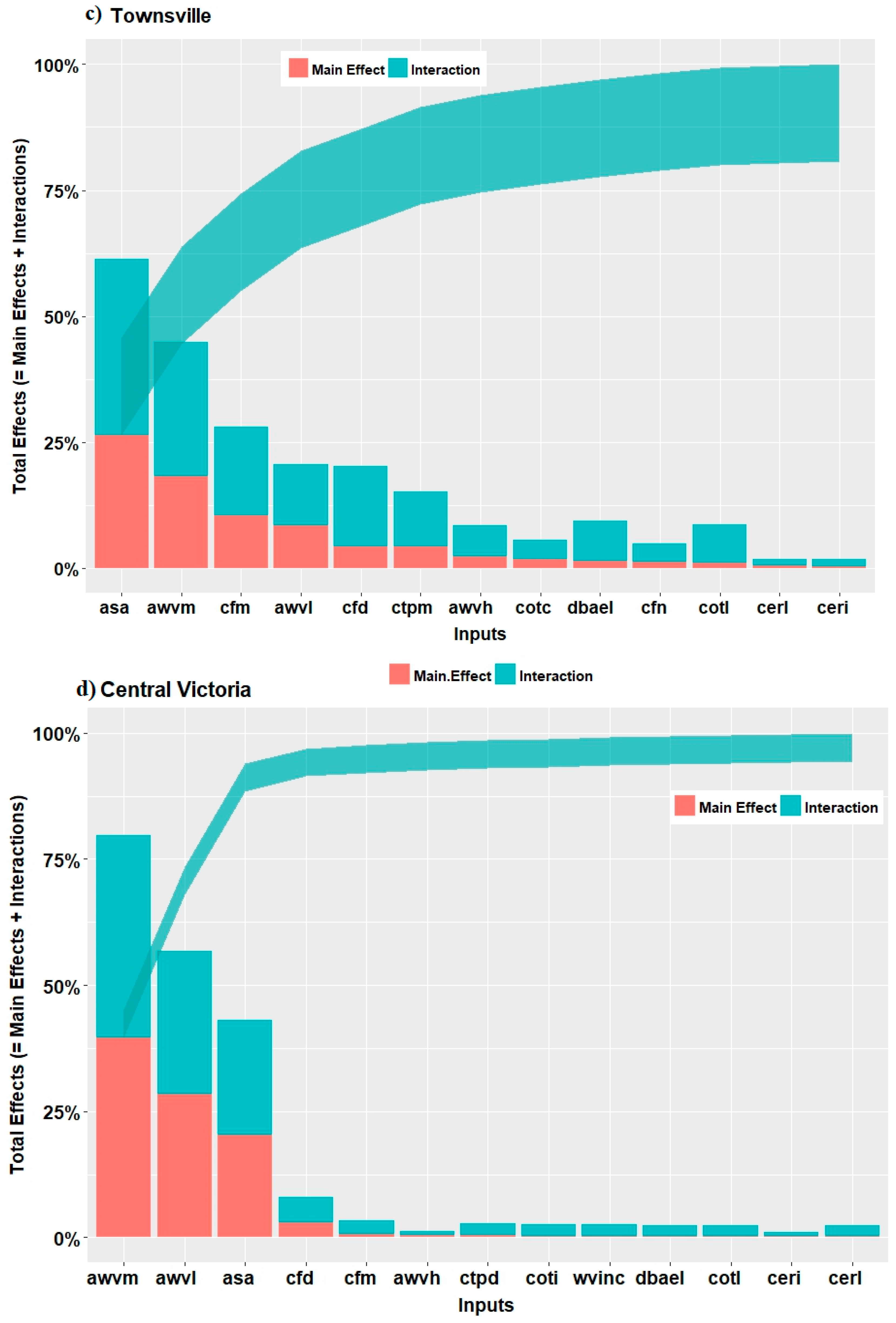
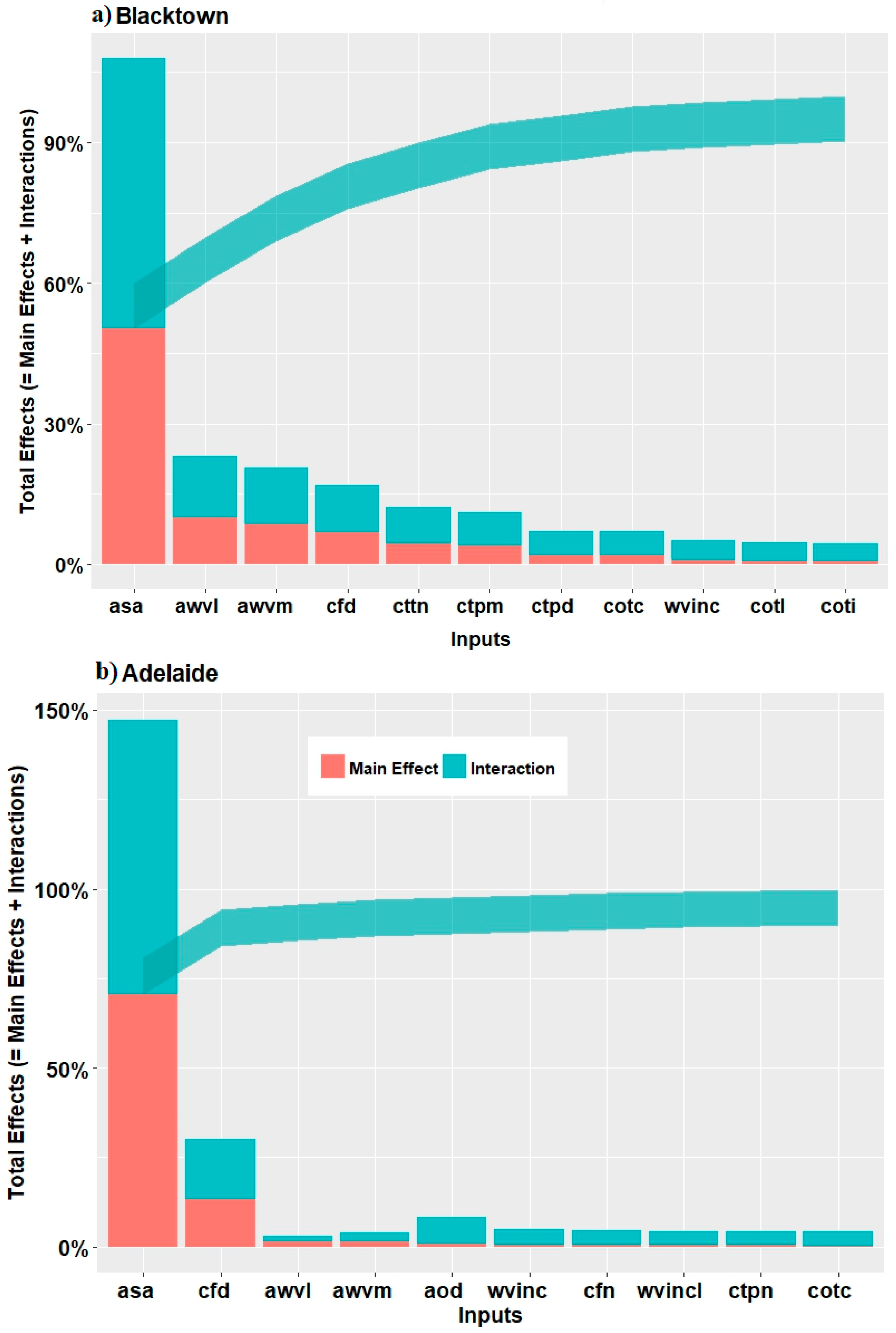
Figure 2 is a “Lowry plot” and shows the relative contribution to the total variance in GSR, from each selected MODIS input. Notably, the vertical bars show ME and TE for each input ranked in order of their main importance, whilst the lower and upper bounds show the cumulative sum of the main and total effect, respectively. This analysis shows that almost 72%, 50% and 27% of the variance in GSR was due to the asa variable (i.e., aerosol scattering angle) for the Adelaide, Blacktown and Townsville study sites, respectively. In contrast, for the case of Central Victoria, almost 40% of the total variance in GSR was due to awvm (i.e., medium atmospheric water vapour) compared to about 23% due to asa. For Adelaide, however, the second highest contribution was derived from day-time cloud fraction (cfd ≈ 27%). It can therefore be concluded that for Adelaide, these input variables are important and are likely to affect the performance of the deep learning models if they are neglected. Similarly, for Central Victoria, the low atmospheric water vapour (awvl), aerosol scattering angle (asa), and day-time cloud fraction (cfd) were found to be the second, third and fourth highest contributors analysed by the GEM-SA method, whereas the other MODIS input variables appeared to have a negligible effect (<5%).

In contrast to the above results, for the case of Blacktown, all of the other MODIS-derived inputs had a negligible effect on GSR with less than 10% of the total variance. It can therefore be concluded that to include 90% of the variance, the first six MODIS parameters (asa, awvl, awvm, cfd and cttn) are required in modelling GSR for Blacktown. Similarly, the first 10 MODIS parameters (asa, awvm cfm, awvl, cfd, ctpm, awvh, cotc and dbael) are required for Townsville to include 90% of the variance. The effect of MODIS inputs on the target variable can be easily identified with the GEM-SA method. As revealed in this analysis, it should be noted that the most important MODIS inputs are not the same for all four locations; hence, a sensitivity analysis of FS-based inputs is necessary to identify more clearly the role of these predictors in modelling the objective variable.

3.3. Deep Learning Predictive Model Design

In this study, deep learning was implemented in Python with the Keras Deep Learning library together with Theano [73] used for modelling GSR in a computer with an Intel core i7 processor @ 3.3 GHz and with 16 GB RAM memory.

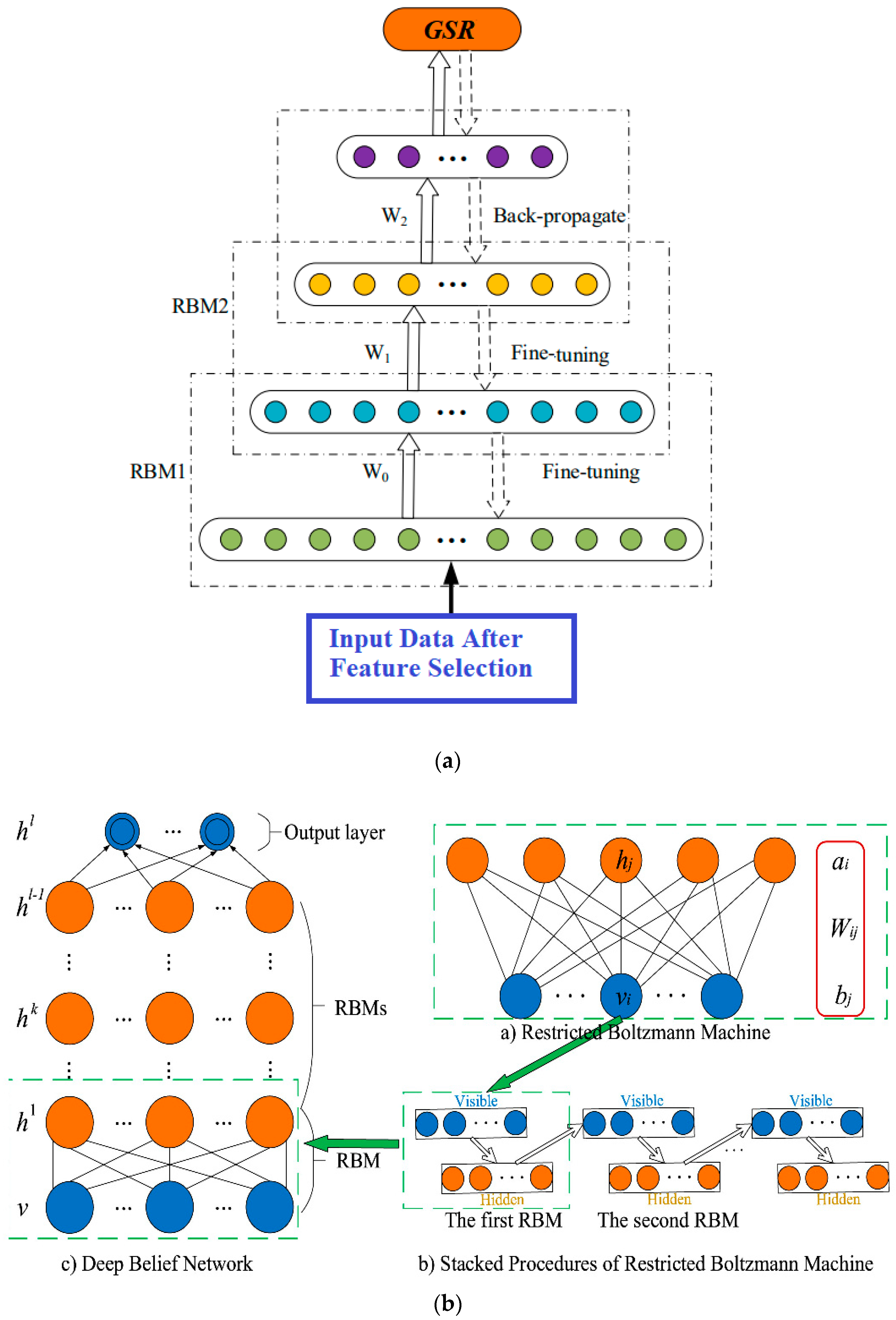
3.3.1. Deep Belief Networks

After a feature selection process and sensitivity analysis of MODIS-derived predictors, a DBN model architecture was designed. This study followed the notion that there is no theoretical basis to set a correct number of layers in a deep learning model. Indeed, insufficient hidden layers means that there could be no proper feature space, resulting in an under-fitted model, but too many layers can lead to the issues of over-fitting, as well as an “ill-posed” problem with higher computational costs [74]. Considering these, a trial and error method was adopted to determine the optimal structure of a DBN model, selected carefully from a total of 12 different neuronal architectures.

For the DBN model, this study used back-propagation for all trained models, but the activation functions were switched between rectified linear unit (ReLU) and the sigmoid equation with a regularization parameter used for fine tuning. The finer details of DBM models are as follows.

(1)

Back-propagation was used to adjust weights, using the derivative chain principle on model errors that were propagated from the last to the first layer. The two parameters implemented were the batch size [2,5] and epochs (100, 200), where training samples were divided into groups of the same size. Notably, the batch size refers to the samples in each group fed to the network before weight updates are performed, whereas epochs are related to the iterations of fine-tuning. Generally, the network can undergo fine-tuning with a smaller batch size or a larger number of epochs [75] including a large iteration set of 1000 in this study.

(2)

To avoid overfitting, a least absolute shrinkage and selection operator (i.e., L2 or lasso regularization) was used to update the cost function by adding a regularization term [76], such that the weights were reduced, to assume a neural network with a smaller weight matrix, leading to a cost-efficient DBN model. This is likely to reduce the overfitting [77], so in this study, we used the L2 regularization as 0.01.

(3)

The learning rate for stacked restricted Boltzmann machine (RBM) and back-propagation were fixed to 0.01 and 0.001 for the DBN model design following earlier studies [78].

In accordance with Table 2, the input nodes were selected by the feature selection algorithm, and hidden layers were deduced by trial and error with analysis of the influence on training performance. As a result, one hidden layer was used at first, and increased up to two layers with variable layers and neurons to optimize the predictive model. This resulted in 12 distinct DBN architectures where the DBN₁₀ model was the optimal model.

Table 3. The influence of feature selection algorithms on GSR prediction problems in terms of the relative root mean square (RRMSE %) generated by the deep belief network (DBN) model for a selected solar city, Adelaide (Australia) in the training phase illustrated as an example. The most optimal feature selection algorithm (i.e., PSO) and the relevant DBN model architectures (i.e., DBN₁₀) are highlighted in blue and is boldface.

Feature Selection Algorithm	DBN1	DBN2	DBN3	DBN4	DBN5	DBN6	DBN7	DBN8	DBN9	DBN10	DBN11	DBN12
ACO	3.8032	3.605	6.0055	4.1061	3.8771	5.9773	3.4115	3.6646	3.7953	4.9275	4.0954	4.9497
EXH	4.6274	4.4285	4.1359	5.7535	6.1618	5.1044	5.4939	6.0681	5.9135	4.4656	6.469	5.4435
FSRNCA	3.7848	4.3611	3.3554	3.2943	4.3768	3.8191	3.7903	5.3001	3.4902	4.0396	4.282	4.9547
GA	5.1471	3.2947	3.5085	3.8677	4.0935	5.5466	3.8229	6.5333	3.8884	3.4569	3.6279	4.0753
MIR	4.7199	4.3303	4.5359	4.3908	5.1334	4.7249	4.969	9.4603	4.8635	4.3226	6.7647	4.5045
NSGA	3.2782	3.3948	4.4819	5.2861	4.1812	3.3408	4.9873	7.3162	4.4266	3.431	3.4871	3.9187
PSO	2.9939	4.9381	8.214	3.0133	4.8548	4.3518	4.6447	3.5864	3.6208	2.9888	4.512	3.2131
Relief	4.7294	4.7415	4.5825	6.0117	5.516	6.0632	4.8268	5.2409	4.3927	4.4404	4.7927	7.5023
RFER	4.2767	3.9111	3.9301	3.8939	4.5415	4.8686	4.4713	5.6978	4.3635	3.9684	4.4727	4.3049
RF	4.4939	5.4009	4.2472	4.293	6.3196	4.6522	4.3344	4.4513	4.678	4.4939	5.1191	4.5643
SA	3.29	3.3942	3.3791	4.0482	4.5882	3.4462	3.7251	3.4854	3.5494	4.0958	4.0854	3.3233
SBR	4.4648	4.339	6.6621	5.3684	4.3839	4.0238	4.1885	4.6828	3.9967	4.4697	5.0949	6.799
SFR	3.4398	3.3889	4.8542	3.7915	4.8091	3.7299	4.4864	4.4268	3.7121	3.1502	4.1725	3.4217
Step	3.4244	3.3991	3.6212	3.3992	4.4455	3.8746	4.0521	3.3514	4.5755	3.457	3.8704	3.6596
UNV	4.6064	5.0044	4.7281	4.293	5.7903	4.6687	5.2329	5.6587	4.7297	4.6151	4.7372	5.0933

lists the effect of feature selection in designing the optimal DBN model, where the relative root mean square (RRMSE %) generated for a selected study site, Adelaide in the model training phase, is illustrated. Evidently, MODIS-based predictors acquired through the particle swarm optimization (PSO) algorithm yielded the lowest RRMSE (≈ 2.98%) in the training DBN₁₀ model, as identified in Table 3.

Similarly (not shown here), the MODIS-derived predictors analysed by the genetic algorithm with DBN₁₁ (RRMSE ≈ 3.25%), analysed with step feature selection for DBN₂ (RRMSE ≈ 3.79%) and the relief algorithm with DBN₂ (RRMSE ≈ 3.71%), yielded the lowest RRMSE compared to the other DBN models for Blacktown, Townsville and Central Victoria, respectively. In addition, the increase in neurons in the hidden layers above 50 was seen to increase training errors for Adelaide, with RRMSE being elevated by 65%, 174%, 81%, 62%, 45%, 55%, 19% and 21% for DBN₂, DBN₃, DBN₄, DBN₅, DBN₆, DBN₇, DBN₈ and DBN₉, respectively (not shown here). In this study, a total of 180 DBN architectures were developed to generate the optimal GSR predictive model.

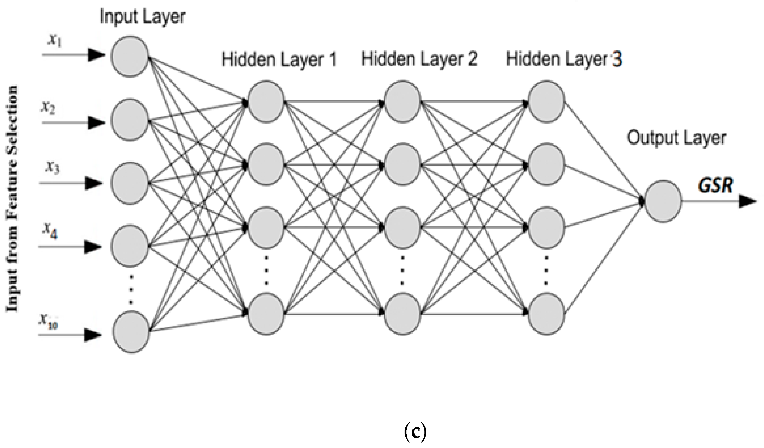
3.3.2. Deep Neural Network

To design a competing deep learning approach for GSR prediction, the next objective model, DNN with 3 hidden layers, 1 input layer where MODIS-derived predictor variables were incorporated from the FS process and 1 output layer corresponding to the target (i.e., GSR), was designed. As with the case of DBN (Section 3.3.1, there appeared to be no preferred method to optimize a DNN model, so a trial and error approach was implemented, where the number of neurons in the hidden layer, activation function, batch size, and number of neurons were tested randomly to satisfy the most accurate GSR model.

Specifically, the modelling experiments were executed 10 times for the same DNN configuration to attain the best result, with the various steps as follows.

• In each trial and error, DNN was trained using popular algorithms: AdaGrad, RMSProp, AdaDelta, Adam, Adamax, Nadam and SGD. It is noteworthy that the Adam algorithm is normally quite popular [79], given it is an enhanced combination of RMSProp and the moments techniques [80]. In this study, we utilized all seven algorithms to determine the optimal DNN architecture.
• To avoid overfitting, three measures were employed. First, we added L2 regularization to penalize the weights in the deep neural network. Second, the dropout technique was used to omit the subset of hidden units at each iteration of a training procedure [81]. Third, early stopping was applied by monitoring the validation performance with the last 10% of the training dataset, in accord with earlier studies [82].

In total, six distinct DNN model architectures with different hyperparameters were developed.

Table 4. The architecture of 6 different DNN designed with the back-propagation algorithm for GSR prediction.

Architecture of DNN
Model	Hidden Layer 1 (H1)	H1 Activation function	Dropout percentage	Activation function	Hidden Layer 2 (H2)	H2 Activation function	Hidden Layer 3 (H3)	H3 Activation function	Batch Size	Epochs
DNN1	500	Sigmoid	0.2	ReLU	200	Sigmoid	500	Sigmoid	1	1000
DNN2	500	Sigmoid	0.2	ReLU	200	Sigmoid	500	Sigmoid	3	1000
DNN3	50	Sigmoid	0.2	ReLU	20	Sigmoid	5	Sigmoid	3	1000
DNN4	500	Sigmoid	0.2	ReLU	50	Sigmoid	20	Sigmoid	3	200
DNN5	100	ReLU	0.2	ReLU	50	ReLU	20	tanh	1	200
DNN6	100	ReLU	0.2	ReLU	50	Sigmoid	20	tanh	5	500
Architecture of Back-propagation (BP) Algorithm for DNN
BP Optimizers for the DNN Model				Learning rate	Epsilon, ε	Decay, δ	Rho, ρ	Beta, β1	Beta, β2
Gradient-based optimization, AdaGrad				0.01	None	0
Geoff Hinton’s adaptive learning rate method, RMSProp				0.001	None	0	0.9	0.9	0.999
Extended AdaGrad algorithm, AdaDelta				1	None	0	0.95	0.9	0.999
Adaptive Moment Estimation, Adam				0.001	None	0
Kingma and Ba, (2015) Adamax				0.002	None	0
Nesterov-accelerated adaptive moment estimation, Nadam				0.002	None	0.004
Stochastic gradient descent, SGD				0.01	None	0
where
δ = Learning rate decay over each update, ρ = Decay factor ε = Factor for updating the variables to eliminate dividing by zero
β1 = The exponential decay rate for the first moment estimates
β2 = The exponential decay rate for the second moment estimates

Note: ReLU and tanh stand for rectified linear units and hyperbolic tangent activation functions, respectively.

shows the architecture for one study site (Central Victoria), where the best model designed with the Adam and SGD algorithms was shown to generate the lowest RRMSE.

3.3.3. Comparison Models

To benchmark the objective deep learning model (i.e., DBN and DNN), this study used the Scikit package [83] to design a Python-based predictive model for GSR with XGBoost [84], gradient boosting regression [85], decision tree [86] and the random forest regressor [87]. For the tuning of the regression model’s hyperparameters, the study used a grid search [88] package where several parameters like the maximum depth of the tree (max_depth), the number of samples required to split an internal node (min_samples_split), the number of features to consider when looking for the best split (max_features) and the others were tuned.

Table 5a,b shows a full list of parameters tuned by the grid search method with 10-fold cross-validation, where the optimal parameter for each of the study sites, yielding the lowest RRMSE, is shown.

For the ANN model, MATLAB 2017b software was utilized [89]. In this study, ANN with various hidden neurons in its hidden layer (1–50) was used with the Levenberg–Marquardt back-propagation algorithm (trainlm) [90] including the hyperbolic tangent and logarithmic sigmoid as activation functions, tested in hidden and output layers, respectively. The ANN model with the low RRMSE and high correlation coefficient (r) was selected.

3.4. Model Performance Criteria

To evaluate the performance of the proposed deep learning models against their comparative counterparts, statistical metrics were employed. Commonly-used metrics like RMSE, MAE and Pearson’s correlation coefficient (r), together with skill score metrics ($RMS{E}_{ss}$) defined in Equation (7) are as follows.

$${RMSE}_{ss}=1-\frac{{RMSE}_{ℳ}}{{RMSE}_{𝒫}}$$

(7)

where $ℳ$ refers to the error (RMSE) obtained in the predicted results employed to assess model performance. Here, $𝒫$ is the RMSE of a persistence model. The persistence model, which is also called the naive predictor, considers that the GSR at t + 1 equals the GSR at t. The interpretation of this metric is that a value of ${RMSE}_{ss}$ close to zero will indicate that the performance of the model is similar to that of the persistence model.

By contrast, if this metric is a positive value, the models under study are likely to outperform the persistence model (which is the baseline), whereas if $RMS{E}_{ss}$ attains a negative value, then the persistence model is likely to be better than the models under study. This study also utilized the normalized performance indicators based on the Nash–Sutcliffe coefficient (E_NS), Willmott’s index (WI) and the Legate’s and McCabe’s index (LM), which provide advanced assessment of models relative to the E_NS and WI values.

In addition to these metrics, this study considered absolute percentage bias (APB) and Kling–Gupta efficiency (KGE) as key performance indicators for GSR prediction. The optimal value of APB is 0.0, with low-magnitude values indicating accurate model simulation; whereas, KGE is a model evaluation criterion that can be decomposed into the contribution of the mean, variance and correlation on model performance [91]. A KGE value of unity is considered as the perfect fit. Similarly, underestimation bias and overestimation bias of models are represented by positive and negative values of APB, respectively.

The mathematical derivation is as follows:

$$E_{NS}=1-\frac{{\sum }_{i=1}^N{\left[GS{R}^m-GS{R}^p\right]}^2}{{\sum }_{i=1}^N{\left[GS{R}^m-〈GS{R}^m〉\right]}^2}$$

(8)

$$WI=1-\frac{{\sum }_{i=1}^N{\left[GS{R}^m-GS{R}^p\right]}^2}{{\sum }_{i=1}^N{\left[|(GS{R}^p-〈GS{R}^m〉)|+|(GS{R}^m-〈GS{R}^m〉)|\right]}^2}$$

(9)

$$LM=1-\frac{{\sum }_{i=1}^N|GS{R}^m-GS{R}^p|}{{\sum }_{i=1}^N|GS{R}^m-〈GS{R}^m〉|}$$

(10)

$$APB=\left[\frac{{\sum }_{i=1}^N(GS{R}^m-GS{R}^p)\ast 100}{{\sum }_{i=1}^{N}GS{R}^m}\right]$$

(11)

$$\begin{array}{l}KGE=1-\sqrt{{(r-1)}^2+{\left(\frac{<GS{R}^p{>}_{}}{<GS{R}^m{>}_{}}-1\right)}^2+{\left(\frac{C{V}_p}{C{V}_m}\right)}^2}\\ \mathrm{where}\\ r=\mathrm{correlation}\mathrm{coeffecient}\\ CV=\mathrm{coefficient}\mathrm{of}\mathrm{variation}\end{array}$$

(12)

where $GS{R}^p$ and $GS{R}^m$ are the predicted (i.e., estimated) and measured values, respectively, and $〈 〉$ refers to the average value of the respective data in the tested set.

4. Results and Discussion

In this section, the results generated by the DBN and DNN algorithms within the testing phase are presented to ascertain the appropriateness of the two deep learning methods used for GSR prediction, tested at diverse sites including Australia’s solar cities. These were also benchmarked against single hidden layer (i.e., ANN) and ensemble models (random forest regression (RF), extreme gradient boosting regression (XGBoost), Gradient Boosting Machine (GBM) and decision trees (DT). It is noteworthy that the results are only presented for DNN₁₀ and DBN₂, the two optimized models in accordance with Table 4 and Table 5.

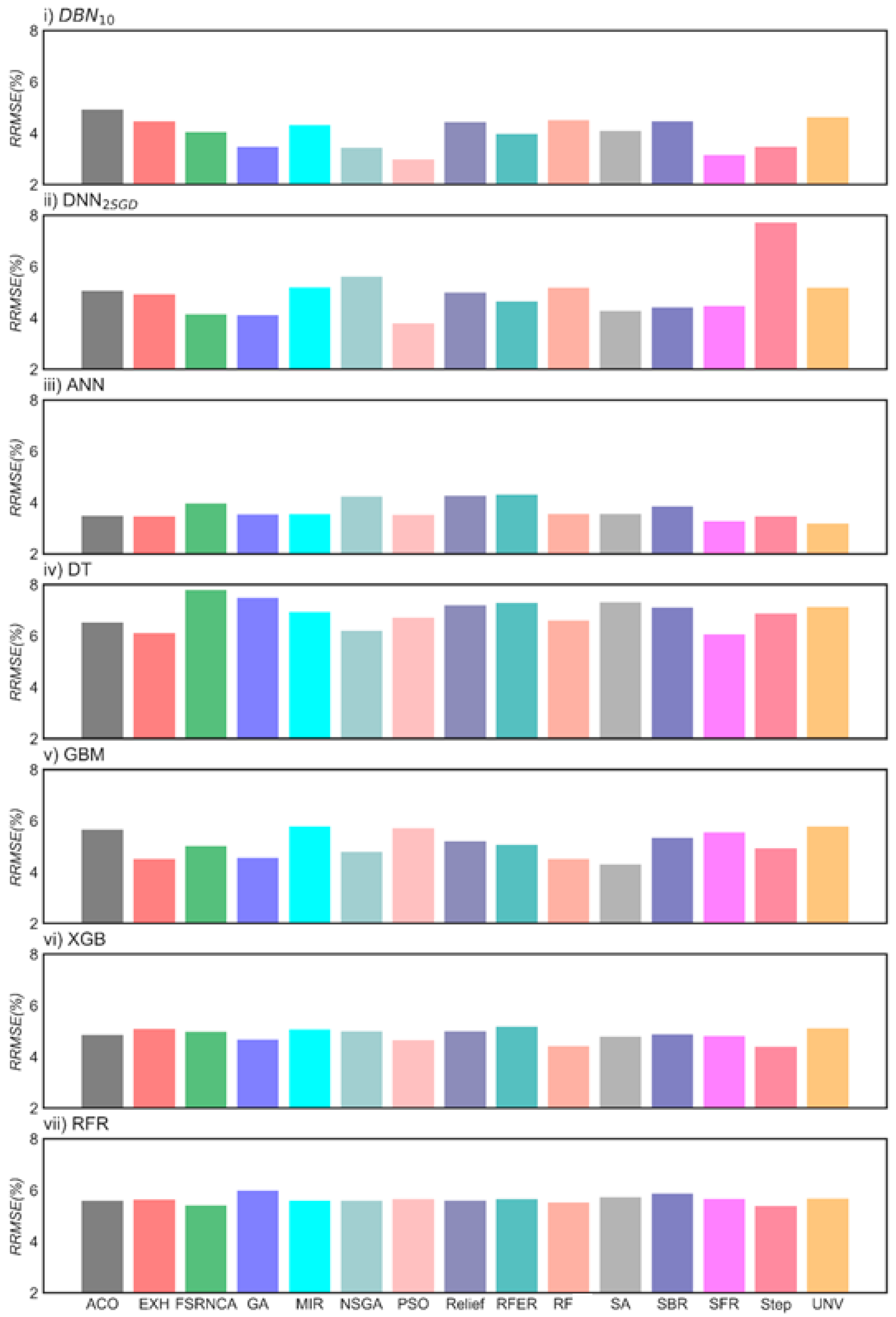
Figure 3 shows this for Adelaide, where the optimal model was selected on the basis of the lowest RRMSE. It should be noted that for this location, the optimized models (DBN₁₀ and DNN₂) (where SGD was used as the back-propagation algorithm) with input selected by the PSO approach were seen to yield a better result. Similarly, for the ANN model, the inputs screened by the nondominated sorting genetic algorithm (NSGA) feature selection approach appeared to be better, and similarly for the DT, GBM, RF and XGB models, inputs screened by the sequential forward selection (SFR), SA, sequential backward selection (SBR), step and NSGA appeared to yield a relatively low RRMSE compared to other feature selection methods.

The model designation is as follows: DBN₁₀ = Deep Belief Network 10, DNN2_SGD = Deep Neural Network 2 with SGD as back-propagation, ANN = neural network, DT = decision tree, RF = random forest regression, GBM = gradient boosting machine and XGBR= extreme gradient boosting regression.

In this study, a feature selection (FS) and sensitivity analysis process utilizing a Lowry plot (Figure 2) were combined to deduce the best FS method for GSR prediction. Note that the nomenclature of any model is designated as FS-(model name), for example, for the Adelaide study site, the model names are designated as PSO-DBN₁₀, PSO-DNN_2SGD, PSO-ANN, PSO-DT, PSO-GBM, PSO-RF and PSO-XGBR. The number that appears after the respective model name, for example, DBN₁₀, is used to represent Deep Belief Network Model Number 10, as deduced from Table 3. Similarly, the subscript (SGD, AdaGrad, Adam) in the model names represent the back-propagation algorithm that was used in training the neural network model. For the ANN, however, only one back-propagation algorithm (LM), the most popular algorithm, was used, so the subscript is not mentioned.

Table 6. Evaluating the training performance of DBN₁₀ and DNN₂ vs. the counterpart models in terms of their best feature selection methods, as measured by the relative root mean squared error (RRMSE, %) used for long-term GSR predictions.

Predictive Model Type	Acronym	Approach for Feature Selection and Performance Error	Australia’s Solar City
			Blacktown	Central Victoria	Adelaide	Townsville
Deep Learning Models	DBN10	Best Feature Selection Algorithm	GA	Relief	PSO	PSO
		RRMSE	3.279	3.7133	2.988	3.791
	DNN2	Best Feature Selection Algorithm	GA	Relief	PSO	EXH
		RRMSE	3.66	4.8296	3.774	3.899
Single Hidden Layer ANN, Decision Tree and Ensembles Models	ANN	Best Feature Selection Algorithm	ACO	FSRNCA	NSGA	NSGA
		RRMSE	4.39	6.252	3.449	4.666
	DT	Best Feature Selection Algorithm	RF	FSRNCA	SFR	Step
		RRMSE	6.49	9.7043	6.055	6.036
	GBM	Best Feature Selection Algorithm	SFR	Relief	SA	RFER
		RRMSE	3.755	6.177	4.302	4.959
	RF	Best Feature Selection Algorithm	ACO	UVR	Step	RFER
		RRMSE	4.884	7.0976	5.375	5.65
	XGBR	Best Feature Selection Algorithm	NSGA	NSGA	Step	RFER
		RRMSE	4.2808	6.3964	4.392	4.644

Note: The best models (DNN₂ and DBN₁₀) are highlighted in blue and boldfaced, and the symbols are as per Table 1 and Table 2a.

shows the training root mean squared error generated for different FS algorithms integrated with deep learning and its respective comparative algorithms, required to select the critical MODIS-derived predictors. In accordance with this evaluation, for the DBN₁₀ model, the GA appeared to be the best FS algorithm for the study site Blacktown, whereas the relief algorithm was the best for the case of Central Victoria, and the PSO algorithm was the best for both the Adelaide and Townsville study sites. However, when the DNN₂ model was evaluated, root mean squared errors were slightly higher for each FS algorithm compared to those obtained from DBN₁₀, but these predictive errors remained much lower than all single hidden layer and ensemble models, thus confirming the superiority of deep learning over the less sophisticated models. When both deep learning models (i.e., DBN₁₀ and DNN₂) were evaluated individually, there appeared to be a clear consensus that the DBN₁₀ model exceeded the performance of DNN₂, used with its best FS approach.

Table 7. Comparison of deep learning models vs. counterpart models. The best model is highlighted in blue and boldfaced (DBN₁₀ represents the optimal model, to accord with Table 3, and DNN_{2 Nadam} represents the optimal model, to accord with Table 5, trained with the Nadam-type back-propagation algorithm.

Australia’s Solar City	Model	r	RMSE (MJ·m−2·day−1)	MAE (MJ·m−2·day−1)	RMSEss
Blacktown	DBN10	0.994	0.546	0.45	0.824
	DNN2Nadam	0.99	0.706	0.503	0.773
	ANN	0.989	0.739	0.536	0.739
	DT	0.955	1.309	0.979	0.579
	RF	0.982	0.798	0.635	0.744
	GBM	0.988	0.664	0.568	0.787
	XGBR	0.985	0.727	0.589	0.766
Adelaide	DBN10	0.997	0.503	0.426	0.863
	DNN2SGD	0.996	0.636	0.546	0.826
	ANN	0.997	0.653	0.529	0.824
	DT	0.985	1.063	0.791	0.713
	RF	0.989	0.895	0.652	0.754
	GBM	0.988	0.906	0.72	0.758
	XGBR	0.992	0.737	0.577	0.801
Central Victoria	DBN10	0.996	0.614	0.498	0.836
	DNN2SGD	0.994	0.798	0.592	0.787
	ANN	0.984	1.276	0.995	0.682
	DT	0.961	1.696	1.217	0.553
	RF	0.984	1.094	0.854	0.714
	GBM	0.988	0.942	0.799	0.753
	XGBR	0.987	0.992	0.825	0.74
Townsville	DBN10	0.974	0.773	0.627	0.718
	DNN2RMSProp	0.967	0.868	0.646	0.682
	ANN	0.972	0.991	0.858	0.641
	DT	0.951	1.181	0.973	0.572
	RF	0.95	1.212	0.971	0.559
	GBM	0.947	1.254	1.006	0.539
	XGBR	0.953	1.205	0.959	0.56
Average of 5 Study Sites	DBN10	0.990	0.609	0.500	0.810
	DNN2RMSProp	0.987	0.752	0.572	0.767
	ANN	0.986	0.915	0.730	0.722
	DT	0.963	1.312	0.990	0.604
	RF	0.976	1.000	0.778	0.693
	GBM	0.978	0.942	0.773	0.709
	XGBR	0.979	0.915	0.738	0.717

compares deep learning models vs. the counterpart models in the testing phase, measured by the correlation coefficient (r), root mean squared error (RMSE), mean absolute error (MAE) and skill score (RMSE_ss). As mentioned earlier, only the optimally-trained models with the lowest MAE and RMSE, the highest r and the RMSE_ss values are shown. Between the deep learning and comparative (SHL and ensemble) models, the DBN model yielded better GSR predictions for all four solar cities. This is evident, for example, when comparing the DBN accuracy statistics (i.e., r ≈ 0.994, RMSE ≈ 0.546 MJ·m⁻²·day⁻¹, MAE ≈ 0.450 MJ·m⁻²·day⁻¹ and RMSE_ss ≈ 0.824 for Blacktown GA-DBN₁₀) with the equivalent ANN and GBM models result statistics (r ≈ 0.989, RMSE ≈ 0.739 MJ m⁻²·day⁻¹, MAE ≈ 0.536 MJ·m⁻²·day⁻¹ and RMSE_ss ≈ 0.739 for Blacktown GA-ANN and r ≈ 0.988, RMSE ≈ 0.664 MJ·m⁻²·day⁻¹, MAE ≈ 0.568 0 MJ·m⁻²·day⁻¹ and RMSE_ss ≈ 0.787 for Blacktown GA-GBM). Comparatively better results for DBN₁₀ models were also seen for all of the other solar cities, confirming the reliability of this deep learning approach, as a viable estimator GSR, with implications for long-term solar energy assessments.

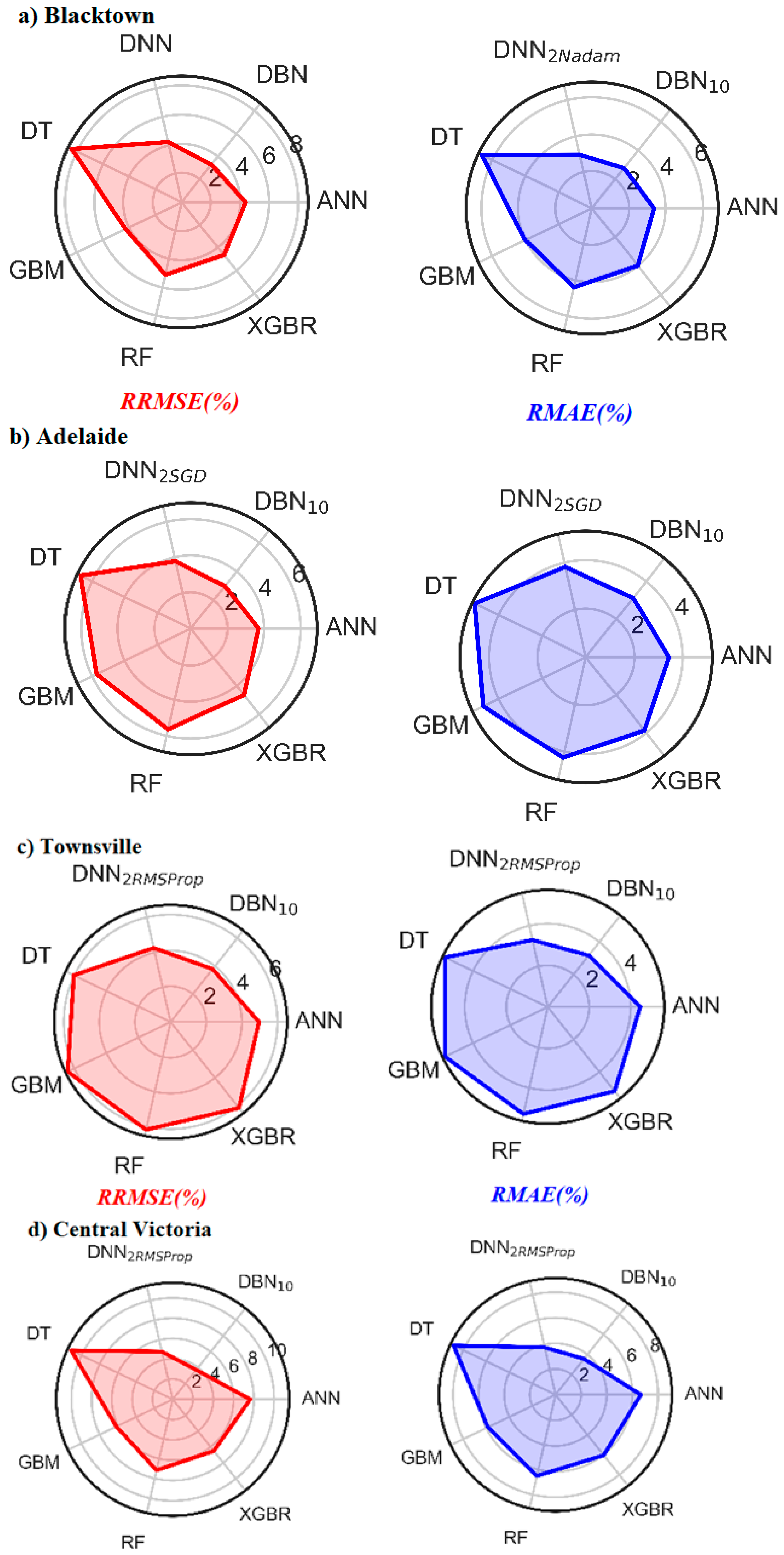
In conjunction with the statistical score metrics, the relative prediction errors were used to show the alternative “goodness-of-fit” for the predicted in relation to the observed GSR data. Figure 4 shows the radar plots in the model’s testing phase for DNN₂ and DBN₁₀ in terms of the RRMSE (%) and RMAE % values. Note that these percentage errors were also used as alternative metrics to enable the model comparison at geographically-diverse sites [92]. It can be seen that the DBN model yielded high precision (with the lowest RRMSE and RMAE) followed by the comparative (SHL and ensemble) models.

For the optimal DBN model, the RRMSE and RMAE were found to be 3.279/2.763%, 2.989/3.124%, 3.713/3.572% and 3.792/3.175% for the study site Blacktown (GA-DBN₁₀), Adelaide (PSO-DBN₁₀), Central Victoria (Relief-DBN₁₀), and Townsville (PSO-DBN₁₀), respectively. On the other hand, the other deep learning model lagged behind the accuracy of DBN with 4.240/2.970%, 3.774/3.825%, 4.830/3.781% and 4.256/3.175% for Blacktown (GA-DNN_2Nadam), Adelaide (PSO-DNN_2SGD), Central Victoria (Relief-DNN_2SGD) and Townsville (PSO-DNN_2RMSProp), showing relatively good performance, compared to the SHL and ensemble models.

The SHL and ensemble models’ performances were lower than those of the DBN and DNN models, except for the study site Adelaide, where the PSO-ANN model (RRMSE/RMAE) was lower (3.702/3.442%) than the DNN model (RRMSE/RMAE ≈ 3.774/3.825%). In accordance with these outcomes, the relative measures concurred on the suitability of deep learning for GSR prediction at all four solar cities selected across Australia.

It is of interest to this study that a numerical quantification of model performance using Willmott’s index (WI), Nash–Sutcliffe (E_NS) and Legates–McCabe’s index (LM) was made where these metrics should ideally be unity for a perfect model. Subsequently, these results (

Table 8. Performance of deep learning models (i.e., DNN₁₀, DBN_2Nadam) with respect to their comparative counterpart models. The best model is highlighted in bold.

Australia’s Solar City	Model	Model Performance Metrics
		WI	ENS	LM
Blacktown	DBN10	0.993	0.987	0.893
	DNN2Nadam	0.989	0.979	0.88
	ANN	0.989	0.977	0.875
	DT	0.944	0.905	0.738
	RF	0.981	0.965	0.83
	GBM	0.986	0.976	0.848
	XGBR	0.984	0.971	0.843
Adelaide	DBN10	0.997	0.995	0.933
	DNN2SGD	0.996	0.991	0.915
	ANN	0.995	0.989	0.907
	DT	0.982	0.968	0.848
	RF	0.987	0.977	0.875
	GBM	0.987	0.977	0.862
	XGBR	0.991	0.985	0.889
Central Victoria	DBN10	0.996	0.992	0.922
	DNN2RMSProp	0.994	0.987	0.908
	ANN	0.984	0.964	0.837
	DT	0.958	0.923	0.773
	RF	0.982	0.968	0.84
	GBM	0.986	0.976	0.851
	XGBR	0.985	0.974	0.846
Townsville	DBN10	0.975	0.949	0.786
	DNN2RMSProp	0.969	0.936	0.78
	ANN	0.965	0.919	0.713
	DT	0.957	0.904	0.699
	RF	0.949	0.898	0.7
	GBM	0.943	0.891	0.689
	XGBR	0.948	0.9	0.703

Note: DBN₁₀ means the DBN model as per Table 3’s configuration, and DNN_2Nadam means the DNN model as per Table 5 with Nadam as the back-propagation algorithm.

) indicated that deep learning is able to attain a dramatic improvement in comparison to SHL and the ensemble model (Table 8).

The highest magnitude of WI ≈ 0.997, E_NS ≈ 0.995 and LM ≈ 0.933 was registered for the Blacktown study site for a GA-DBN₁₀ model. Intriguingly, the lowest value of WI ≈ 0.943, E_NS ≈ 0.891 and LM ≈ 0.689 was registered at the Townsville study site for the PSO-RF model. Further, the GA-DBN₁₀ model noted the increment in WI, E_NS and LM by 5.2%, 9.06% and 21.02%, respectively, compared to the counterpart (SHL and ensemble) models for the Blacktown study site. A similar trend was also demonstrated for the other solar cities. Hence, it is evident that a deep learning model has a better potential to predict GSR over long-term periods.

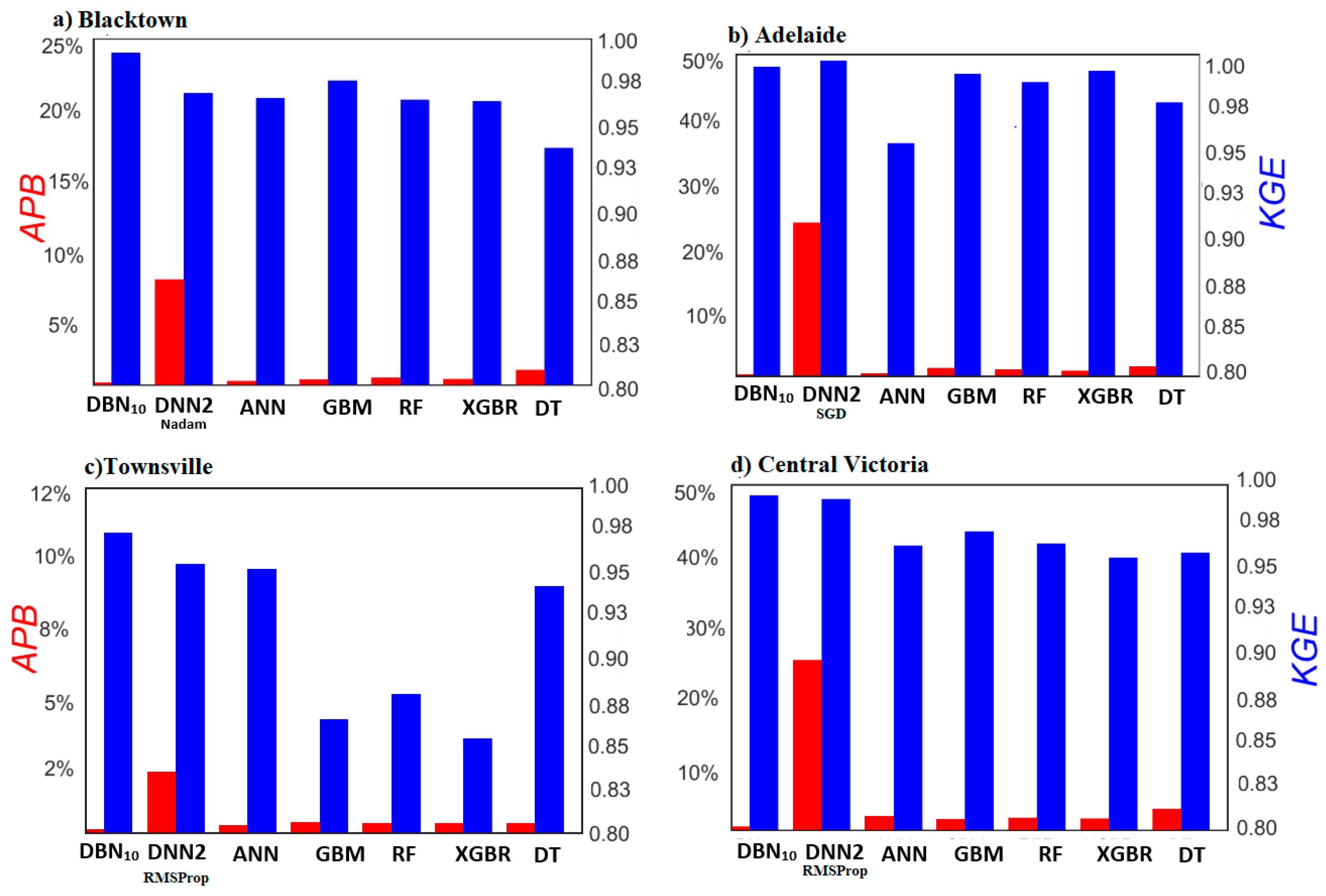
In this paper, a comprehensive evaluation of the deep learning approach for GSR predictions was made in terms of the absolute percentage bias (APB, %) and Kling–Gupta efficiency (KGE) in the testing phase (Figure 5). The evaluation of KGE and APB for these solar cities showed that the DBN₁₀ model constituted the best performing approach.

For example, KGE ≥ 0.99 and APB ≤ 0.025 for the case of Blacktown (GA-DBN₁₀), Adelaide (PSO-DBN₁₀), Central Victoria (Relief-DBN₁₀) and Townsville (PSO-DBN₁₀). Indeed, this plot shows that the magnitude of KGE was oriented toward unity, and the magnitude of APB was oriented toward zero for all deep learning models for all solar cities in consideration. Concurrent with the earlier findings, the deep learning model can be considered as a trustworthy and powerful tool for the prediction of long-term GSR, at least by the evidence generated so far.

Further insights were gained by checking the correspondence between the predicted and actual GSR. Comparing the prescribed deep learning models with an earlier study using wavelet support vector machine models (W-SVM) [14] applied in Australia, it became evident that the precision of the present model was relatively good for prediction of daily averaged monthly global solar radiation. In fact, in that study, their W-SVM model for the Townsville study produced a regression line equation GSR_pred = 0.849 × GSR_obs + 3.02, whereas the present deep learning model generated GSR_pred = 0.969 × GSR_obs + 0.678 and GSR_pre = 0.939 × GSR_obs + 1.196 for DBN (PSO-DBN₁₀) and DNN (PSO-DNN_2RMSProp), respectively. It is therefore clear that the prescribed approaches exceeded the performance of earlier studies.

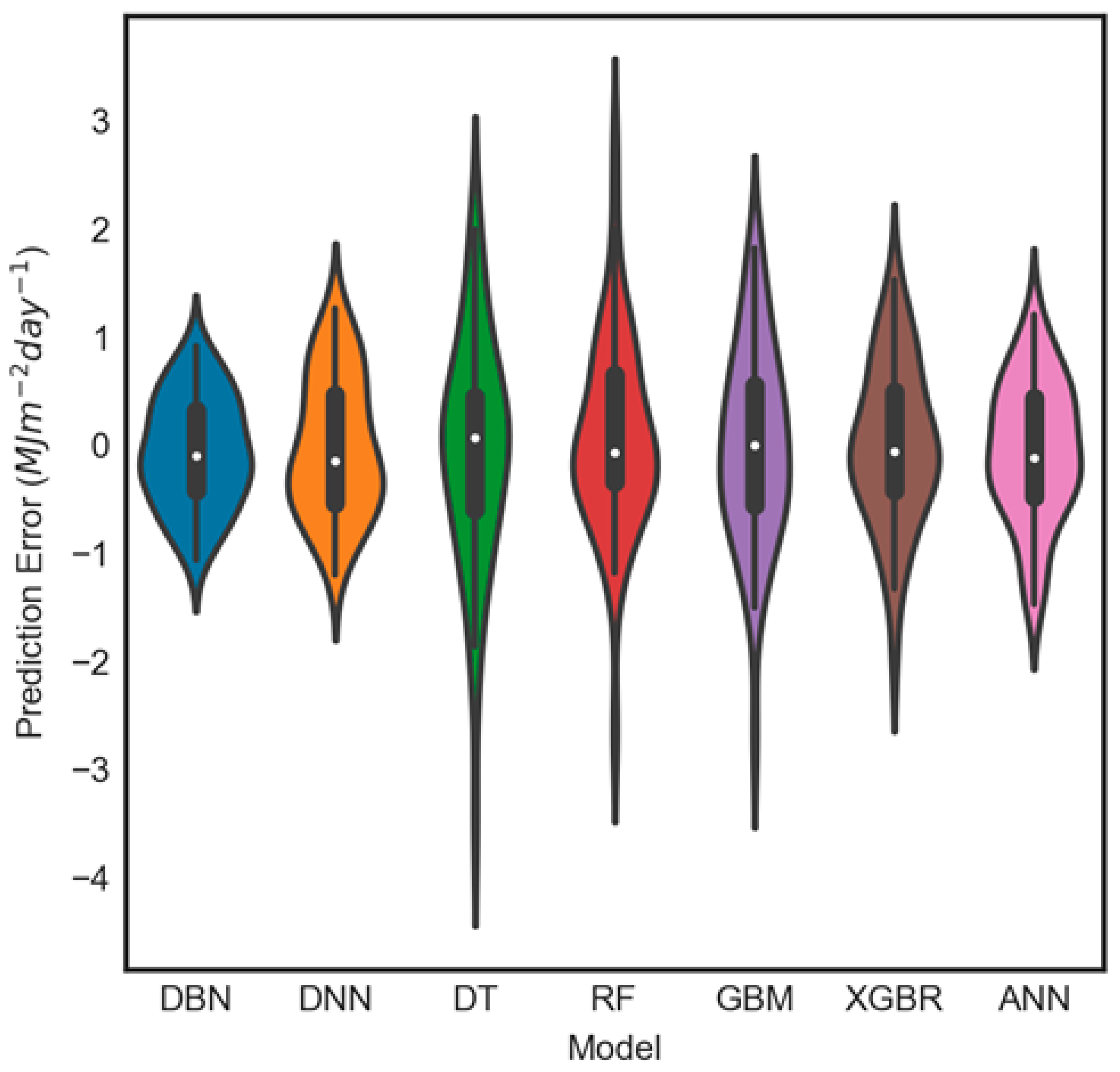
To assess a model’s stability for predicting GSR, the spread of the prediction errors is illustrated with the help of a violin plot [92] (Figure 6). In plotting this, all of the sites’ actual and predicted GSR were considered. It should be noted that a violin plot is a synergistic combination of a box plot and density trace that is rotated and placed on each side to show the distribution shape of these data. The interquartile range is represented by a thick black bar in the centre, whereas 95% confidence intervals are represented by the thin black line or whisker, and the median is represented by the dot.

The shape of the violin displays the frequencies of the values. As can be seen on the figure (Figure 6) with a wider section of the plot, the prediction error (PE) generated by the DBN model had a high probability of a value of zero as compared to the benchmark models. Likewise, the median error (white dot) for a deep learning model was lower than that of comparative (SHL and ensemble) models, and the shape of distribution (extremely thin on each end and wide in the middle) indicates that the PE of DBN were highly concentrated around the median. Overall, it is noteworthy that the DBN model enjoyed superior performance relative to its comparative (SHL and ensemble) models tested for all four Australian solar cities.

To draw a more conclusive argument on the suitability of the deep learning model for GSR prediction,

Table 9. The percentage frequency of the absolute prediction errors, |PE|, in different error bands in the testing phase, encountered by the deep learning model within respect to its comparative counterpart models: a single hidden layer neural network (ANN) and ensemble models for Australia’s solar cites. The best model is highlighted in blue/bold.

Prediction Error, |PE| (%)	Adelaide				Blacktown				Townsville				Central Victoria
	DBN	DNN	ANN	XGBR	DBN	DNN	ANN	XGBR	DBN	DNN	ANN	XGBR	DBN	DNN	ANN	XGBR
0 ⩽ |PE| < 4	86.40	88.60	84.10	79.60	88.60	84.10	84.10	79.50	81.00	81.00	78.30	72.60	81.80	79.50	86.40	84.10
4 ⩽ |PE| < 5	11.40	4.60	4.60	11.40	2.30	11.40	4.60	11.40	7.10	14.30	12.20	12.20	11.40	11.40	2.30	11.40
5 ⩽ |PE| < 6	2.30	6.80	9.10	4.60	6.80	0.00	2.30	6.80	9.50	0.00	7.10	8.10	4.60	4.60	9.10	2.30
|PE| > 6	0.00	0.00	2.30	4.60	2.3	4.60	9.10	2.30	2.40	4.80	2.40	7.10	2.30	4.6	2.30	2.30

shows the prediction error (%), with its respective normalized frequency of the datum points, in each error bracket tested for each of the four solar cities. The normalized frequency is presented as a percentage of the predicted points in each error bracket in terms of the total data points in the testing period. Consistent with the earlier results, the most accurate prediction was obtained by using a deep learning model as the PE (%) attained the maximum value for the lowest range (e.g., Townsville ≈ 81 % (DBN and DNN) within [0 ⩽ |PE| < 4]) compared to the comparative (SHL and ensemble) models (e.g., Townsville ≈ 72.3 % (XGBR) within [0 ⩽ |PE| < 4]).

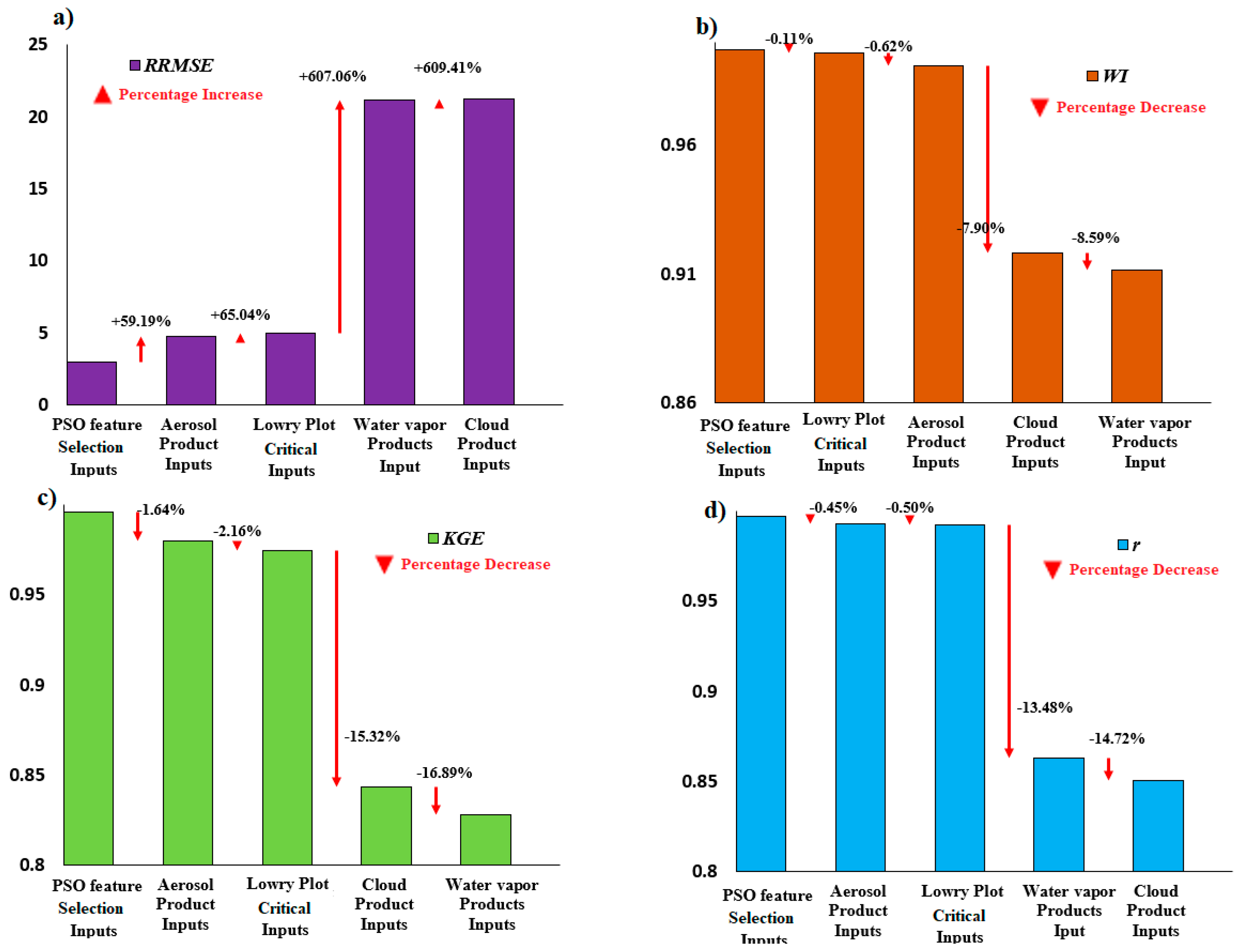
In Figure 7, the sensitiveness of clouds, water vapour and aerosols (i.e., the three main contributors to the fluctuations in global solar radiation) including these GEM-SA critical parameters (Lowry plot, Figure 2) as the predictors of GSR are explored more closely for the case of the Adelaide study site. The four DBN models were tested with the cloud parameters (i.e., cfd, cfn, cotc, cotl, ctpm and cttd), aerosol parameters (asa and aod), atmospheric water vapour (awvl and awvm) and GEM-SA critical parameters (asa, cfd, awvl, and awvm) to arrive at conclusive arguments. The model results were compared with the original model PSO-DBN₁₀ (Table 3).

From the graph (Figure 7), it is deduced that the PSO feature selection gave the best prediction with the lowest RRMSE and the highest values of KGE, WI and r. When only aerosol products from the MODIS data repository were used as a potential input, the RRMSE appeared to increase by 65%, whereas the WI, KGE and r-values decreased by 66.8%, 67% and 66.9%, respectively. Similarly, with the cloud and water vapour product as a potential input, the RRMSE increased much greater than 600%, and KGE, WI and r decreased by more than 70%.

Furthermore, with only four critical parameters from GEM-SA (Lowry plot, asa, cfd, awvl and awvm) as an input, the RRMSE was lower than that of the aerosol, cloud and water vapour product as a potential input. Therefore, it is evident that the cloud and aerosol products were very important predictors and should not be neglected, for GSR predictions at the selected study sites.

5. Further Discussion

5.1. Comprehensive Evaluation of the Deep Learning Approach

It appears that DBN, DNN and also the ANN model (where the first two were designed with a deep learning approach, whereas the third model was designed with a single hidden layer neuronal system) have attained a better accuracy in comparison with all other data-driven models. As far as the error measurements were concerned, the r, however, was based on a linear relationship between observed and predicted GSR and, therefore, can be limited in its capacity to provide a robust model since it standardizes the observed and predicted means and variances [13]. However, RMSE and MAE, used in this study, can provide information about the predictive skill, whereas RMSE measures the goodness-of-fit relevant to high values, and MAE is not weighted towards high(er) magnitude or low(er) magnitude, but instead evaluates all deviations from observed, in both an equal manner and regardless of sign [9]. It is for this reason that all of these metrics were used to evaluate the deep learning models for GSR prediction.

It is important to note that while RMSE can assess the model with higher skill compared to the correlation coefficient, this metric is computed on squared differences [9]. Thus, performance assessment is biased in favour of the peaks and high(er) magnitude events that will in most cases exhibit the greatest error and be insensitive to low(er) magnitude sequences [14]. Consequently, the RMSE can be more sensitive than other performance metrics.

To overcome this issue, in this study, relative errors, root mean squared error (RRMSE) and mean absolute error (RMAE) (Figure 6) were utilized to describe the model over the range of statistically-different GSR, making it possible to compare the models evaluated for geographically- (and climatically-) diverse sites, where MAE and RMSE alone do not make sense. Notably, although the r (≥0.98) value was similar for DBN, DNN and ANN, in terms of RRMSE and RMAE, DBN and DNN outperformed all of the other models. Furthermore, KGE was quite high (≥97.5%) (Figure 7) for the DBN model for all locations as compared to DNN, ANN and the other models. Note that KGE gives more weight to the mismatch between observed and predicted GSR for high GSR because it squares the difference. Additionally, APB was low (≤3%) for DBN, measuring the tendency of predicted GSR to be larger or smaller than observations.

Comprehensively considering the prediction accuracy in terms of RRMSE, RMAE, KGE and APB of deep learning models, the DBN model can be of high utility for predicting long-term GSR using remote sensing data under different climatic conditions in Australia and, perhaps, elsewhere with similar climatic conditions.

5.2. Comparison with Related Research Work

In spite of good performance attained by deep learning approaches, as evidenced by statistical metrics and visual analysis, we further evaluated the models with respect to results from other studies. One such study was the work of [44] that validated a DBN model for daily GSR predictions in the Lhasa region in China using weather station fields (i.e., wind speed, sunshine duration, air dry-bulb temperature, air relative humidity) for the period 1994–2015. In concurrence with the present study (Table 7), that study also concluded that the DBN approach constituted the best model as it generated a relatively low mean absolute bias error, RMSE and a high r-value (i.e., 1.2709 MJ m⁻² day⁻¹, 1.6765 MJ m⁻² day⁻¹ and 0.960).

Further comparison can be made in terms of another relevant study [93] where a DNN model was employed to estimate daily GSR over 30 stations in Turkey. The astronomical factor, extra-terrestrial radiation and climatic variables, sunshine duration, cloud cover, minimum temperature and maximum temperature, were used as input variables with data from 34 stations spanning from 2001–2007 used for training and testing the models. Their proposed DNN model yielded a high coefficient of determination (r² = 0.980) and low RMSE (0.780 MJ m⁻² day⁻¹) and MAE (0.610 MJ m⁻² day⁻¹), which stands within the range of the present study (Table 7).

The results from two latest research works were, however, the closest available comparison of deep learning models for GSR prediction. When directly comparing the prediction metrics, our DBN model outperformed by a noticeable margin, with a lower RMSE (≤ 0.503 MJ·m⁻²·day⁻¹) and MAE (≤ 0.426 MJ·m⁻²·day⁻¹) and high r (≥0.994) values (Table 7). Moreover, the two recent research projects used weather station data (ground-based), whereas the present study used freely-available remote sensing data as potential inputs (Table 2). Furthermore, a feature selection and sensitivity analysis of the MODIS predictors were not performed in the compared research works, whereas this study used fifteen feature selection algorithms (Table 2a) including the GEM-SA method for sensitivity analysis of the MODIS-derived predictors.

In terms of using deep learning models for GSR prediction in Australia, this study is the first of its kind to demonstrate the merits of this algorithm with respect to a neural network model used previously (e.g., ANN). For example, a study by Deo and Sahin [13] that utilized MODIS land surface temperature within an ANN model for long-term GSR predictions and generated an average RMSE of 1.23 MJ·m⁻² over a group of seven sites in regional Queensland had errors far exceeding a current lower average RMSE of 0.609 MJ·m⁻². Furthermore, that study had generated an average MAE of 1.02 MJ·m⁻² in contrast to a lower error value of 0.50 MJ·m⁻².

The comparison shows that the proposed study can be considered as a significant advancement over earlier studies performed in Australia that have used satellite-derived variables, but did not apply deep learning. In this context, a deep learning approach may be adopted for long-term solar radiation modelling and future solar energy exploration.

5.3. Recommendation for Further Research

This study supports the significant merits of a deep learning predictive model to attain greater precision in predicting long-term GSR. Further, the study also provided a significant guideline for selecting appropriate models for GSR prediction in terms of the predictive accuracy in different climatic zones in Australia and also may be applicable elsewhere where similar climatic conditions prevail around the world. However, the scope of this study was restricted in terms of the prediction horizon, authenticating deep learning for monthly averaged, daily GSR, i.e., long-term period.

6. Conclusions

Deep learning models were developed for Australia’s solar cities (i.e., Adelaide, Blacktown, Townsville, and Central Victoria) to estimate long-term GSR. These cities are heterogeneously distributed and represent a significant variation in their climatic conditions. In order to predict the monthly averaged daily GSR as an output, publicly-available MODIS satellite data (aerosol, cloud and water vapour) from GIOVANNI were extracted as the most relevant predictors. Fifteen different wrapper and filter-based feature selection algorithms were applied, with sensitivity analysis of all MODIS-derived predictors using GEM-SA to select the optimum input for the prediction of GSR. The data were segregated 80% for training, and 20% data were used for testing. A total of 180 deep belief networks (12 DBN models, 15 feature selections) and 630 deep neural network models were developed for each site. The developed models were benchmarked with single hidden layer and ensemble models including neural network, gradient boosting machine, extreme gradient boosting regression, decision tree and random forest regression models.

A holistic evaluation via statistical metrics and diagnostic plots revealed that the DBN model generated superior prediction in comparison with the benchmark models (viz., ANN, GBM, XGBR, DT and RF). The site comparison showed that the DBN model had the best performance at Blacktown (Table 7) with the lowest RRMSE ≈ 2.988% and RMAE ≈ 2.76% and highest r ≈ 0.994 and RMSE_ss ≈ 0.824 in predicting GSR. Similarly, the DBN model outperformed all the benchmark models for all sites (Figure 5) in terms of absolute percentage bias and Kling–Gupta efficiency (e.g., KGE ≈ 0.992 and APB ≈ 0.027 for Blacktown using the DBN model, KGE ≈ 0.855 and APB ≈ 0.049 for Townsville using the XGBR model). Furthermore, the regression plot of actual versus predicted GSR demonstrated that, with a slope closer to unity and an intercept closer to zero, the DBN was best in GSR estimation and even outperformed the previous study [93] using a W-SVM model for GSR estimation at Townsville. In addition to this, the sensitivity analysis of the predictor variables demonstrated that aerosol, cloud, and water vapour parameters as input parameters played a significant role in the prediction of GSR (Figure 7). This is a clearly understandable finding, as cloud and aerosol have obvious noticeable effects on sky brightness during daylight hours.

The findings of this study ascertained that with appropriate feature selection (such as PSO, GA and GEM-SA for sensitivity analysis), the deep learning model effectively captured the nonlinear dynamics and interactions amongst the input parameters and GSR in generating optimally-combined and -stabilized predictions for all four study sites. The DL model yielded good results for estimating monthly averaged daily GSR, either better than or comparable to many previous studies reported in the literature. One can conclude that the method derived here can be implemented as a suitable alternative and be successfully applied to similar regions.

References

1. Roda, C.; Chitnis, K.; Peterson, J.; Schwaderer, J. Town- [email protected] J. Home Energy Management System 2014. Available online: https://www.researchgate.net/publication/274780353_Home_Energy_Management_System (accessed on 19 June 2019).
2. Liu, Y.; Qiu, B.; Fan, X.; Zhu, H.; Han, B. Review of smart home energy management systems. Energy Procedia 2016, 104, 504–508. [Google Scholar] [CrossRef]
3. Kumar, S.; Kaur, T. Development of ANN based model for solar potential assessment using various meteorological parameters. Energy Procedia 2016, 90, 587–592. [Google Scholar] [CrossRef]
4. Sivaneasan, B.; Yu, C.Y.; Goh, K.P. Solar forecasting using ANN with fuzzy logic Pre-processing. Energy Procedia 2017, 143, 727–732. [Google Scholar] [CrossRef]
5. Ghritlahre, H.K.; Prasad, R.K. Application of ANN technique to predict the performance of solar collector systems—A review. Renew. Sustain. Energy Rev. 2018, 84, 75–88. [Google Scholar] [CrossRef]
6. Ayet, A.; Tandeo, P. Nowcasting solar irradiance using an analog method and geostationary satellite images. Sol. Energy 2018, 164, 301–315. [Google Scholar] [CrossRef] [Green Version]
7. Al-Musaylh, M.S.; Deo, R.C.; Adamowski, J.F.; Li, Y. Short-term electricity demand forecasting with MARS, SVR and ARIMA models using aggregated demand data in Queensland, Australia. Adv. Eng. Inform. 2018, 35, 1–16. [Google Scholar] [CrossRef]
8. Al-Musaylh, M.S.; Deo, R.C.; Adamowski, J.F.; Li, Y. Two-phase particle swarm optimized-support vector regression hybrid model integrated with improved empirical mode decomposition with adaptive noise for multiple-horizon electricity demand forecasting. Appl. Energy 2018, 17, 422–439. [Google Scholar] [CrossRef]
9. Deo, R.C.; Sahin, M.; Adamowski, J.; Mi, J. Universally deployable extreme learning machines integrated with remotely sensed MODIS satellite predictors over Australia to forecast global solar radiation: A new approach. Renew. Sustain. Energy Rev. 2019, 104, 235–261. [Google Scholar] [CrossRef]
10. Ghimire, S.; Deo, R.C.; Downs, N.J.; Raj, N. Global solar radiation prediction by ANN integrated with European Centre for medium range weather forecast fields in solar rich cites of queensland Australia. J. Clean. Prod. 2019, 216, 288–310. [Google Scholar] [CrossRef]
11. Salcedo-Sanz, S.; Deo, R.C.; Cornejo-Bueno, L.; Camacho-Gómez, C.; Ghimire, S. An efficient neuro-evolutionary hybrid modelling mechanism for the estimation of daily global solar radiation in the Sunshine State of Australia. Appl. Energy 2018, 209, 79–94. [Google Scholar] [CrossRef]
12. Ghimire, S.; Deo, R.C.; Downs, N.J.; Raj, N. Self-adaptive differential evolutionary extreme learning machines for long-term solar radiation prediction with remotely-sensed MODIS satellite and reanalysis atmospheric products in solar-rich cities. Remote Sens. Environ. 2018, 212, 176–198. [Google Scholar] [CrossRef]
13. Deo, R.C.; Sahin, M. Forecasting long-term global solar radiation with an ANN algorithm coupled with satellite-derived (MODIS) land surface temperature (LST) for regional locations in Queensland. Renew. Sustain. Energy Rev. 2017, 72, 828–848. [Google Scholar] [CrossRef]
14. Deo, R.C.; Wen, X.; Feng, Q. A wavelet-coupled support vector machine model for forecasting global incident solar radiation using limited meteorological dataset. Appl. Energy 2016, 168, 568–593. [Google Scholar] [CrossRef]
15. Gutierrez-Corea, F.-V.; Manso-Callejo, M.-A.; Moreno-Regidor, M.-P.; Manrique-Sancho, M.-T. Forecasting short-term solar irradiance based on artificial neural networks and data from neighboring meteorological stations. Sol. Energy 2016, 134, 119–131. [Google Scholar] [CrossRef]
16. Azadeh, A.; Maghsoudi, A.; Sohrabkhani, S. An integrated artificial neural networks approach for predicting global radiation. Energy Convers. Manag. 2009, 50, 1497–1505. [Google Scholar] [CrossRef]
17. Li, L.-L.; Cheng, P.; Lin, H.-C.; Dong, H. Short-term output power forecasting of photovoltaic systems based on the deep belief net. Adv. Mech. Eng. 2017, 9. [Google Scholar] [CrossRef] [Green Version]
18. Liu, H.; Mi, X.-W.; Li, Y.-F. Wind speed forecasting method based on deep learning strategy using empirical wavelet transform, long short term memory neural network and Elman neural network. Energy Convers. Manag. 2018, 156, 498–514. [Google Scholar] [CrossRef]
19. Hinton, G.E.; Salakhutdinov, R.R. Reducing the dimensionality of data with neural networks. Science 2006, 313, 504–507. [Google Scholar] [CrossRef] [PubMed]
20. Xu, W.; Peng, H.; Zeng, X.; Zhou, F.; Tian, X.; Peng, X. Deep belief network-based AR model for nonlinear time series forecasting. Appl. Soft Comput. 2019, 77, 605–621. [Google Scholar] [CrossRef]
21. Torres, J.F.; Fernández, A.; Troncoso, A.; Martínez-Álvarez, F. Deep learning-based approach for time series forecasting with application to electricity load. In Proceedings of the International Work-Conference on the Interplay Between Natural and Artificial Computation, Corunna, Spain, 19–23 June 2017. [Google Scholar]
22. Qin, M.; Li, Z.; Du, Z. Red tide time series forecasting by combining ARIMA and deep belief network. Knowl. Based Syst. 2017, 125, 39–52. [Google Scholar] [CrossRef]
23. Kuremoto, T.; Kimura, S.; Kobayashi, K.; Obayashi, M. Time series forecasting using a deep belief network with restricted Boltzmann machines. Neurocomputing 2014, 137, 47–56. [Google Scholar] [CrossRef]
24. Huang, H.B.; Li, R.X.; Yang, M.L.; Lim, T.C.; Ding, W.P. Evaluation of vehicle interior sound quality using a continuous restricted Boltzmann machine-based DBN. Mech. Syst. Signal Process. 2017, 84, 245–267. [Google Scholar] [CrossRef] [Green Version]
25. Lara-Fanego, V.; Ruiz-Arias, J.A.; Pozo-Vázquez, D.; Santos-Alamillos, F.J.; Tovar-Pescador, J. Evaluation of the WRF model solar irradiance forecasts in Andalusia (southern Spain). Sol. Energy 2012, 86, 2200–2217. [Google Scholar] [CrossRef]
26. Yadav, A.K.; Chandel, S.S. Solar radiation prediction using Artificial Neural Network techniques: A review. Renew. Sustain. Energy Rev. 2014, 33, 772–781. [Google Scholar] [CrossRef]
27. Qazi, A.; Fayaz, H.; Wadi, A.; Raj, R.G.; Rahim, N.A.; Khan, W.A. The artificial neural network for solar radiation prediction and designing solar systems: A systematic literature review. J. Clean. Product. 2015, 104, 1–12. [Google Scholar] [CrossRef]
28. Mohanty, S.; Patra, P.K.; Sahoo, S.S. Prediction and application of solar radiation with soft computing over traditional and conventional approach—A comprehensive review. Renew. Sustain. Energy Rev. 2016, 56, 778–796. [Google Scholar] [CrossRef]
29. Davy, R.J.; Troccoli, A. Interannual variability of solar energy generation in Australia. Sol. Energy 2012, 86, 3554–3560. [Google Scholar] [CrossRef]
30. Weiss, A.J.; Hays, C.; Hu, Q.; Easterling, W. Incorporating bias error in calculating solar irradiance: Implications for crop yield simulations. Agron. J. 2001, 93, 1321–1326. [Google Scholar] [CrossRef]
31. Deo, R.C.; Downs, N.; Adamowski, J.; Parisi, A. Adaptive Neuro-Fuzzy inference system integrated with solar zenith angle for forecasting sub-tropical photosynthetically active radiation. Food Energy Secur. 2018, 8, e00151. [Google Scholar] [CrossRef]
32. Antonopoulos, V.Z.; Papamichail, D.M.; Aschonitis, V.G.; Antonopoulos, A.V. Solar radiation estimation methods using ANN and empirical models. Comput. Electron. Agric. 2019, 160, 160–167. [Google Scholar] [CrossRef]
33. Prasad, R.; Ali, M.; Kwan, P.; Khan, H. Designing a multi-stage multivariate empirical mode decomposition coupled with ant colony optimization and random forest model to forecast monthly solar radiation. Appl. Energy 2019, 236, 778–792. [Google Scholar] [CrossRef]
34. Persson, C.; Bacher, P.; Shiga, T.; Madsen, H. Multi-site solar power forecasting using gradient boosted regression trees. Sol. Energy 2017, 150, 423–436. [Google Scholar] [CrossRef]
35. Fan, J.; Wang, X.; Wu, L.; Zhou, H.; Zhang, F.; Yu, X.; Lu, X.; Xiang, Y.Z. Comparison of support vector machine and extreme gradient boosting for predicting daily global solar radiation using temperature and precipitation in humid subtropical climates: A case study in China. Energy Convers. Manag. 2018, 164, 102–111. [Google Scholar] [CrossRef]
36. Abuella, M.; Chowdhury, B. Forecasting of solar power ramp events: A post-processing approach. Renew. Energy 2019, 133, 1380–1392. [Google Scholar] [CrossRef]
37. Thushara, D.S.M.; Hornberger, G.M.; Baroud, H. Decision analysis to support the choice of a future power generation pathway for Sri Lanka. Appl. Energy 2019, 240, 680–697. [Google Scholar] [CrossRef]
38. Tao, Y.; Chen, H.; Qiu, C. Wind power prediction and pattern feature based on deep learning method. In Proceedings of the Power and Energy Engineering Conference (APPEEC), Hong Kong, China, 7–10 December 2014. [Google Scholar]
39. Khodayar, M.; Teshnehlab, M. Robust deep neural network for wind speed prediction. In Proceedings of the 4th Iranian Joint Congress on Fuzzy and Intelligent Systems (CFIS), Zahedan, Iran, 9–11 September 2015. [Google Scholar]
40. Qureshi, A.S.; Khan, A.; Zameer, A.; Usman, A. Wind power prediction using deep neural network based meta regression and transfer learning. Appl. Soft Comput. 2017, 58, 742–755. [Google Scholar] [CrossRef]
41. Wang, H.-Z.; Li, G.-Q.; Wang, G.-B.; Peng, J.-C.; Jiang, H.; Liu, Y.-T. Deep learning based ensemble approach for probabilistic wind power forecasting. Appl. Energy 2017, 188, 56–70. [Google Scholar] [CrossRef]
42. He, Y.; Deng, J.; Li, H. Short-term power load forecasting with deep belief network and copula models. In Proceedings of the 9th International Conference on Intelligent Human-Machine Systems and Cybernetics (IHMSC), Hangzhou, China, 26–27 August 2017. [Google Scholar]
43. Hinton, G.E. A practical guide to training restricted boltzmann machines. In Neural Networks: Tricks of the Trade; Springer: Berlin, Germany, 2012; pp. 599–619. [Google Scholar]
44. Wang, M.; Zang, H.; Cheng, L.; Wei, Z.; Sun, G. Application of DBN for estimating daily solar radiation on horizontal surfaces in Lhasa, China. Energy Procedia 2019, 158, 49–54. [Google Scholar] [CrossRef]
45. Lin, Y.; Liu, H.; Xie, G.; Zhang, Y. Time series forecasting by evolving deep belief network with negative correlation search. In Proceedings of the 2018 Chinese Automation Congress (CAC), Xi’an, China, 30 November–2 December 2018. [Google Scholar]
46. Benali, L.; Notton, G.; Fouilloy, A.; Voyant, C.; Dizene, R. Solar radiation forecasting using artificial neural network and random forest methods: Application to normal beam, horizontal diffuse and global components. Renew. Energy 2019, 132, 871–884. [Google Scholar] [CrossRef]
47. Qiao, J.; Li, S.; Li, W. Mutual information based weight initialization method for sigmoidal feedforward neural networks. Neurocomputing 2016, 207, 676–683. [Google Scholar] [CrossRef]
48. Kingma, D.P.; Ba, J. Adam: A method for stochastic optimization. arXiv 2014, arXiv:14126980. [Google Scholar]
49. Tieleman, T.; Hinton, G. Lecture 6.5-rmsprop: Divide the gradient by a running average of its recent magnitude. COURSERA Neural Netw. Mach. Learn. 2012, 4, 26–31. [Google Scholar]
50. Duchi, J.; Hazan, E.; Singer, Y. Adaptive subgradient methods for online learning and stochastic optimization. J. Mach. Learn. Res. 2011, 12, 2121–2159. [Google Scholar]
51. Dozat, T. Incorporating Nesterov Momentum into Adam. 2016. Available online: https://openreview.net/forum?id=OM0jvwB8jIp57ZJjtNEZ (accessed on 19 June 2019).
52. Zeiler, M.D. Adadelta: An Adaptive Learning Rate Method. 2012. Available online: https://arxiv.org/abs/1212.5701 (accessed on 19 June 2019).
53. Ismail, M.; Attari, M.; Habibi, S.; Ziada, S. Estimation theory and neural networks revisited: REKF and RSVSF as optimization techniques for deep-learning. Neural Netw. 2018, 108, 509–526. [Google Scholar] [CrossRef] [PubMed]
54. Zahedi, A. Solar PV for Australian tropical region; the most affordable and an appropriate power supply option. In Proceedings of the 2016 Australasian Universities Power Engineering Conference (AUPEC), Brisbane, Australia, 25–28 September 2016. [Google Scholar]
55. Şenkal, O. Solar radiation and precipitable water modeling for Turkey using artificial neural networks. Meteorol. Atmos. Phys. 2015, 127, 481–488. [Google Scholar] [CrossRef]
56. Bisht, G.; Bras, R.L. Estimation of net radiation from the MODIS data under all sky conditions: Southern Great Plains case study. Remote Sens. Environ. 2010, 114, 1522–1534. [Google Scholar] [CrossRef]
57. Morshed, A.; Aryal, J.; Dutta, R. Environmental Spatio-temporal Ontology for the Linked Open Data Cloud. In Proceedings of the 12th IEEE International Conference on Trust, Security and Privacy in Computing and Communications, Melbourne, Australia, 16–18 July 2013. [Google Scholar]
58. Chen, C.; Jiang, H.; Zhang, Y.; Wang, Y. Investigating spatial and temporal characteristics of harmful Algal Bloom areas in the East China Sea using a fast and flexible method. In Proceedings of the 18th International Conference on Geoinformatics, Beijing, China, 18–20 June 2010. [Google Scholar]
59. Acker, J.; Soebiyanto, R.; Kiang, R.; Kempler, S. Use of the NASA Giovanni data system for geospatial public health research: Example of weather-influenza connection. ISPRS Int. J. Geo-Inf. 2014, 3, 1372–1386. [Google Scholar] [CrossRef]
60. Chen, J.-L.; Xiao, B.-B.; Chen, C.-D.; Wen, Z.-F.; Jiang, Y.; Lv, M.-Q.; Wu, S.-J.; Li, G.-S. Estimation of monthly-mean global solar radiation using MODIS atmospheric product over China. J. Atmos. Sol. Terr. Phys. 2014, 110, 63–80. [Google Scholar] [CrossRef]
61. Yang, C.; Xu, Q.; Xu, X.; Zeng, P.; Yuan, X. Generation of solar radiation data in unmeasurable areas for photovoltaic power station planning. In Proceedings of the 2014 IEEE PES General Meeting Conference Exposition, Chicago, IL, USA, 14–17 April 2014. [Google Scholar]
62. Meenal, R.; Selvakumar, A.I. Review on artificial neural network based solar radiation prediction. In Proceedings of the 2nd International Conference on Communication and Electronics Systems (ICCES), Tamilnadu, India, 19–20 October 2017. [Google Scholar]
63. Wang, K.; Qi, X.; Liu, H.; Song, J. Deep belief network based k-means cluster approach for short-term wind power forecasting. Energy 2018, 165, 840–852. [Google Scholar] [CrossRef]
64. Prasad, R.; Deo, R.C.; Li, Y.; Maraseni, T. Ensemble committee-based data intelligent approach for generating soil moisture forecasts with multivariate hydro-meteorological predictors. Soil Tillage Res. 2018, 181, 63–81. [Google Scholar] [CrossRef]
65. Guyon, I.; Elisseeff, A. An introduction to variable and feature selection. J. Mach. Learn. Res. 2003, 3, 1157–1182. [Google Scholar]
66. Rodriguez-Galiano, V.F.; Luque-Espinar, J.A.; Chica-Olmo, M.; Mendes, M.P. Feature selection approaches for predictive modelling of groundwater nitrate pollution: An evaluation of filters, embedded and wrapper methods. Sci. Total Environ. 2018, 624, 661–672. [Google Scholar] [CrossRef] [PubMed]
67. Lal, T.N.; Chapelle, O.; Weston, J.; Elisseeff, A. Embedded methods. In Feature Extraction; Springer: New York, NY, USA, 2006; pp. 137–165. [Google Scholar]
68. Guyon, I.; Elisseeff, A. An introduction to feature extraction. In Feature Extraction; Springer: New York, NY, USA, 2006; pp. 1–25. [Google Scholar]
69. Hilario, M.; Kalousis, A. Approaches to dimensionality reduction in proteomic biomarker studies. Brief. Bioinform. 2008, 9, 102–118. [Google Scholar] [CrossRef] [PubMed]
70. Kennedy, M.C.; Petropoulos, G.P. Chapter 17— GEM-SA: The Gaussian Emulation Machine for Sensitivity Analysis. In Sensitivity Analysis in Earth Observation Modelling; Petropoulos, G.P., Srivastava, P.K., Eds.; Elsevier: Amsterdam, The Netherlands, 2017; pp. 341–361. [Google Scholar]
71. O’Hagan, A. Bayesian analysis of computer code outputs: A tutorial. Reliab. Eng. Syst. Saf. 2006, 91, 1290–1300. [Google Scholar] [CrossRef]
72. Gant, S.E.; Kelsey, A.; McNally, K.; Witlox, H.W.; Bilio, M. Methodology for global sensitivity analysis of consequence models. J. Loss Prev. Process Ind. 2013, 26, 792–802. [Google Scholar] [CrossRef]
73. Al-Rfou, R.; Alain, G.; Almahairi, A.; Angermueller, C.; Bahdanau, D.; Ballas, N.; Bastien, F.; Bayer, J.; Belikov, A.; Belopolsky, A.; et al. Theano: A Python framework for fast computation of mathematical expressions. arXiv 2016, arXiv:1605.02688. [Google Scholar]
74. Zheng, J.; Fu, X.; Zhang, G. Research on exchange rate forecasting based on deep belief network. Neural Comput. Appl. 2019, 31, 573–582. [Google Scholar] [CrossRef]
75. Feng, W.; Wu, S.; Li, X.; Kunkle, K. A Deep Belief Network Based Machine Learning System for Risky Host Detection. 2017. Available online: https://arxiv.org/abs/1801.00025 (accessed on 19 June 2019).
76. Han, S.; Pool, J.; Tran, J.; Dally, W. Learning both weights and connections for efficient neural network. In Proceedings of the Advances in Neural Information Processing Systems, Montreal, QC, Canada, 7–12 December 2015. [Google Scholar]
77. Ng, A.Y. Feature selection, L 1 vs. L 2 regularization, and rotational invariance. In Proceedings of the Twenty-First International Conference on Machine Learning (ACM), Banff, AB, Canada, 4–8 July 2014. [Google Scholar]
78. Kamada, S.; Ichimura, T. An adaptive learning method of Deep Belief Network by layer generation algorithm. In Proceedings of the Region 10 Conference (TENCON), Marina Bay Sands, Singapore, 22–25 November 2016. [Google Scholar]
79. Reddy, B.K.; Delen, D. Predicting hospital readmission for lupus patients: An RNN-LSTM-based deep-learning methodology. Comput. Biol. Med. 2018, 101, 199–209. [Google Scholar] [CrossRef]
80. Kinga, D.; Adam, J.B. A method for stochastic optimization. In Proceedings of the International Conference on Learning Representations (ICLR), San Diego, CA, USA, 7–9 May 2015. [Google Scholar]
81. Mai, F.; Tian, S.; Lee, C.; Ma, L. Deep learning models for bankruptcy prediction using textual disclosures. Eur. J. Oper. Res. 2018, 274, 743–758. [Google Scholar] [CrossRef]
82. Dahl, G.E.; Sainath, T.N.; Hinton, G.E. Improving deep neural networks for LVCSR using rectified linear units and dropout. In Proceedings of the Acoustics, Speech and Signal Processing (ICASSP), Vancouver, BC, Canada, 26–30 May 2013. [Google Scholar]
83. Pedregosa, F.; Varoquaux, G.; Gramfort, A.; Michel, V.; Thirion, B.; Grisel, O.; Blondel, M.; Prettenhofer, P.; Weiss, R.; Dubourg, V.; et al. Scikit-learn: Machine learning in Python. J. Mach. Learn. Res. 2011, 12, 2825–2830. [Google Scholar]
84. Chen, T.; Guestrin, C. Xgboost: A scalable tree boosting system. In Proceedings of the 22nd ACM Sigkdd International Conference on Knowledge Discovery and Data Mining (ACM), California, CA, USA, 13–17 August 2016. [Google Scholar]
85. Prettenhofer, P.; Louppe, G. Gradient Boosted Regression Trees in Scikit-Learn. 2014. Available online: https://orbi.uliege.be/handle/2268/163521 (accessed on 19 June 2019).
86. Xia, Y.; Liu, C.; Li, Y.; Liu, N. A boosted decision tree approach using Bayesian hyper-parameter optimization for credit scoring. Expert Syst. Appl. 2017, 78, 225–241. [Google Scholar] [CrossRef]
87. Lakshminarayanan, B.; Roy, D.M.; Teh, Y.W. Mondrian forests: Efficient online random forests. In Proceedings of the Advances in Neural Information Processing Systems, Montreal, QC, Canada, 8–13 December 2014. [Google Scholar]
88. Komer, B.; Bergstra, J.; Eliasmith, C. Hyperopt-sklearn: Automatic hyperparameter configuration for scikit-learn. In Proceedings of the Scientific Computing with Python, Austin, TX, USA, 6–12 July 2014. [Google Scholar]
89. Demuth, H.; Beale, M. Matlab Neural Network Toolbox User’s Guide Version 6; The MathWorks Inc.: Natick, MA, USA, 2009. [Google Scholar]
90. Rego, A.S.C.; Valim, I.C.; Vieira, A.A.S.; Vilani, C.; Santos, B.F. Optimization of sugarcane bagasse pretreatment using alkaline hydrogen peroxide through ANN and ANFIS modelling. Bioresour. Technol. 2018, 267, 634–641. [Google Scholar] [CrossRef] [PubMed]
91. Kling, H.; Gupta, H. On the development of regionalization relationships for lumped watershed models: The impact of ignoring sub-basin scale variability. J. Hydrol. 2009, 373, 337–351. [Google Scholar] [CrossRef]
92. Hintze, J.L.; Nelson, R.D. Violin plots: A box plot-density trace synergism. Am. Stat. 1998, 52, 181–184. [Google Scholar]
93. Kaba, K.; Sarıgül, M.; Avcı, M.; Kandırmaz, H.M. Estimation of daily global solar radiation using deep learning model. Energy 2018, 162, 126–135. [Google Scholar] [CrossRef]
Figure 1. (a) Deep belief network algorithm flow chart. (b) The procedures to implement the deep belief network. (c) Topological structure of the deep neural network (DNN). RBM, restricted Boltzmann machine; GSR, global solar radiation.
Energies 12 02407 g001aEnergies 12 02407 g001b
Figure 2. Lowry plot with the main (primary) and the total cumulative effects of MODIS-derived predictors employed to predict monthly averaged daily global solar radiation GSR.
Energies 12 02407 g002aEnergies 12 02407 g002b
Figure 3. Relative root mean square error (RRMSE %) in the model’s testing phase, illustrated for a selected solar city, Adelaide, to identify the accurate performance using different feature selection algorithms. Note: For acronyms and model names, refer to Table 1, Table 2 and Table 3 and Table 5.
Energies 12 02407 g003
Figure 4. Radar plots in the model’s testing phase for prediction of GSR, in terms of the relative root mean squared error (RRMSE %) and relative mean absolute error (RMAE %).
Energies 12 02407 g004
Figure 5. Bar chart showing a comparison of the optimal deep learning models (i.e., DBN10 and DNN2RMSProp) in terms of their absolute percentage bias (APB, %) and the Kling–Gupta efficiency (KGE) in the testing phase. For notations and model names, please refer to Table 1, Table 2, Table 3, Table 5 and Table 7).
Energies 12 02407 g005
Figure 6. Violin plots of the prediction error (PE) generated by deep learning models (i.e., DBN10 and DNN2Nadam) compared with single hidden layer neuronal and decision tree-based models in the testing phase.
Energies 12 02407 g006
Figure 7. Sensitivity analysis of the relevant MODIS satellite-derived inputs variables: aerosol, cloud and water vapour, in terms of their: (a) relative root mean squared error (RRMSE), (b) Willmott’s index (WI), (c) Kling–Gupta efficiency, (KGE), and (d) correlation coefficient (r).
Energies 12 02407 g007