Forecasting of Coal Demand in China Based on Support Vector Machine Optimized by the Improved Gravitational Search Algorithm

Abstract

The main target of the energy revolution in the new period is coal, but the proportion of coal in primary energy consumption will gradually decrease. As coal is a major producer and consumer of energy, analyzing the trend of coal demand in the future is of great significance for formulating the policy of coal development planning and driving the revolution of energy sources in China. In order to predict coal demand scientifically and accurately, firstly, the index system of influencing factors of coal demand was constructed, and the grey relational analysis method was used to select key indicators as input variables of the model. Then, the kernel function of SVM (support vector machine) was optimized by taking advantage of the fast convergence speed of GSA (gravitational search algorithm), and the memory function and boundary mutation strategy of PSO (particle swarm optimization) were introduced to improve the gravitational search algorithm, and the improved GSA (IGSA)–SVM prediction model was obtained. After that, the effectiveness of IGSA–SVM in predicting coal demand was further proven through empirical and comparative analysis. Finally, IGSA–SVM was used to forecast China’s coal demand in 2018–2025. According to the forecasting results, relevant suggestions about coal supply, consumption, and transformation are put forward, providing scientific basis for formulating an energy development strategy.

1. Introduction

The coal industry is an important basic industry related to national economic and energy security. At the stage of high-quality development, the environment of coal industry development is more complex, and the problems of unbalanced, uncoordinated, and unsustainable development are still outstanding. With the acceleration of the energy revolution, the proportion of coal in primary energy consumption will gradually decrease, but the main energy status will not change for a long time in China [1]. Coal has made irreplaceable contributions to the growth of the national economy. The shortage and surplus of coal supply will seriously interfere with the normal operation of the national economy.

As coal is a major producer and consumer of energy, due to the lack of scientific planning, the imbalance between supply and demand has been affecting the healthy development of the coal industry and national economy for a long time in China. At the same time, given the dominance of coal in China’s energy structure, it is the leading source of carbon dioxide emissions. Thus, the change in coal demand is closely related to China’s low-carbon and clean energy transition. Therefore, the timely adjustment of energy strategic planning with the help of scientific and accurate prediction of coal demand will not only help the coal industry to achieve the balance between supply and demand but also play an important role in promoting the establishment of modern energy systems and realizing the energy revolution.

In order to study the operation rules and characteristics of coal and guide the healthy and sustainable development of the coal industry, it is necessary to focus on the influencing factors of coal demand and coal demand forecasting. Coal demand forecasting is a very complex system. Rational estimation of each component of coal demand will be affected and restricted by many factors. The accuracy of coal demand forecasting depends on the detailed consumption data of major coal-consuming industries and the scientificness of forecasting methods and models. This paper chose the improved gravity search algorithm to optimize the parameters of the support vector machine algorithm and then used the optimized algorithm to predict the values of key factors. This improved intelligent algorithm model can greatly improve the prediction accuracy. The innovations of this article are as follows:

(1)

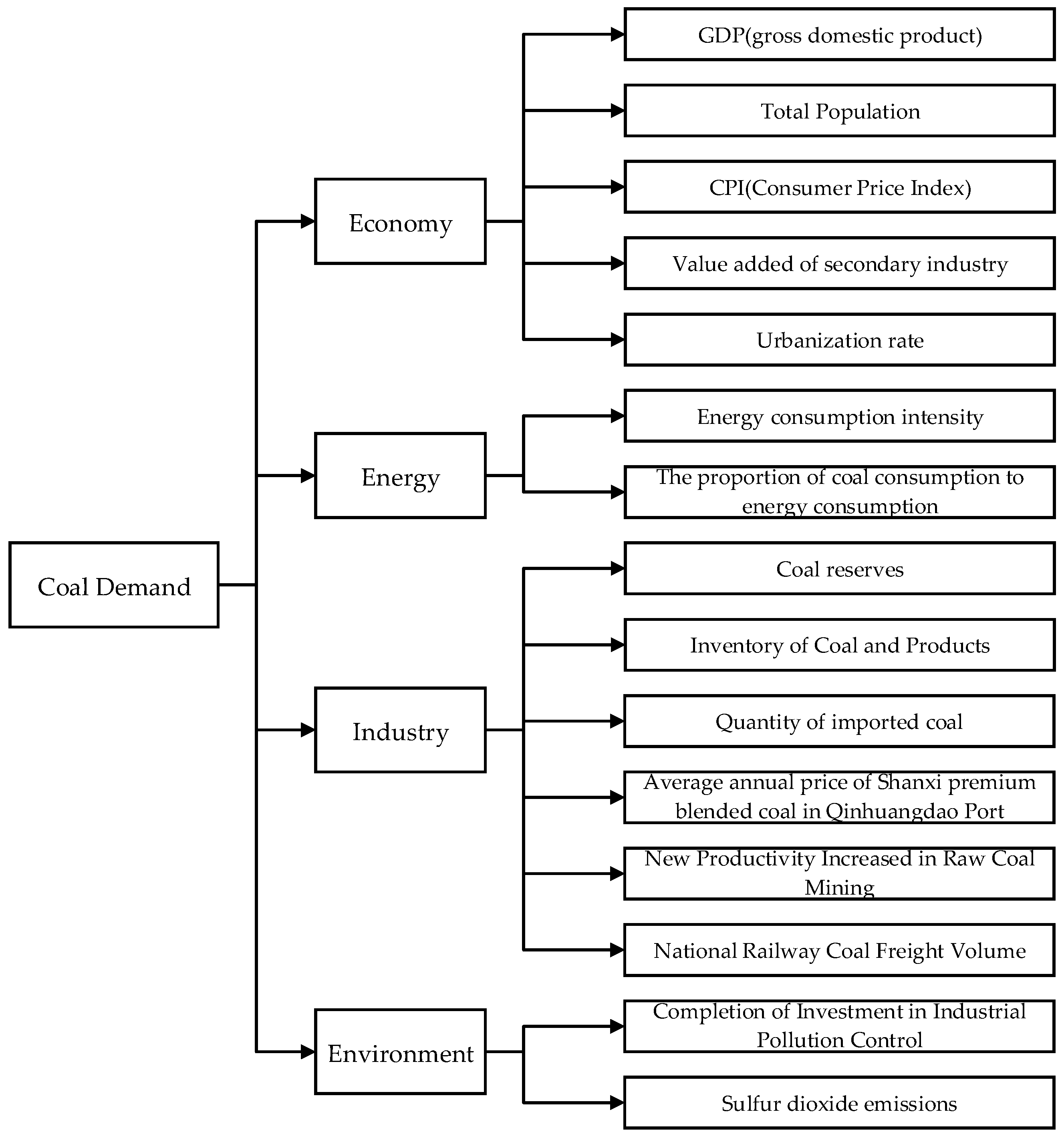
In the analysis of the influencing factors of coal demand, combined with the actual situation of coal production and consumption, economic, social, and environmental constraints, this paper systematically selected 15 impact indicators from the four dimensions of economy, energy, industry, and environment. The grey correlation method was used to select the key indicators as the input variables of the forecasting model.

(2)

Forecasting of coal demand based on the improved gravitational search algorithm–support vector machine (IGSA–SVM). Compared to the traditional optimization algorithm, GSA has the characteristics of fast convergence and strong pioneering performance when optimizing SVM. By introducing the memory function and boundary mutation strategy of particle swarm optimization, it avoids falling into the local optimum when GSA optimizes the parameters of SVM.

The remainder of this study is organized as follows. Section 2 mainly presents some literature related to coal demand forecasting and methods for energy demand forecasting. Section 3 screens the main influencing factors based on grey relational analysis and presents the IGSA–SVM adopted in this paper. The effectiveness of IGSA–SVM in predicting coal demand is further proven by comparing the errors of back propagation (BP), SVM, GSA–SVM, and IGSA–SVM in predicting coal demand, and IGSA–SVM is used to forecast China’s coal demand in 2018–2025 in Section 4. Finally, we summarize the conclusions of this paper and put forward several recommendations in Section 5.

2. Relevant Literature Review

This section summarizes the relevant research from two aspects: coal demand forecasting and energy methods for energy demand forecasting.

2.1. Relevant Research on Coal Demand Forecasting

Coal demand forecasting is a complex system engineering involving economy, energy, and the environment. Scholars’ research mainly focuses on two aspects: influencing factors of demand and coal demand forecasting.

In terms of influencing factors of coal demand, Michieka and Fletcher [2] used the vector autoregressive model and modified Granger causality test to study the relationship between urban population, gross domestic product (GDP), electricity output, and coal consumption. Chong et al. [3] used the logarithmic average Dirichlet decomposition method and found that rapid economic development is the biggest driving factor for the growth of coal consumption, and the improvement of coal utilization efficiency is the main factor to restrain the growth of coal consumption. Kulshreshtha [4] believes that economic development has a great impact on coal consumption. When Lin Boqiang [5] studied the deviation between China’s coal demand growth and economic growth, he believed that technological progress, coal quality change, energy structure adjustment, industrial structure change, environmental governance, and carbon dioxide emissions were the important reasons for the change of coal demand.

In terms of coal demand forecasting, including direct forecasting and indirect forecasting, direct prediction is to get the change of coal consumption through the development and change of various departments which mainly consume coal resources. Reference [6] presented the formulation of forecasting models to get the total coal consumption by forecasting the coal consumption of different sectors in India, including domestic, transportation, and electricity. Reference [7] chose exponential smoothing (ETS) and the Holt–Winters model and used R language software to predict coal consumption in seven major coal-consuming industries. The indirect forecasting method is to construct the model by estimating the internal relationship between coal demand and its driving factors, so as to provide reference for coal demand forecasting. Reference [8] constructed an inverted U-shaped environmental Kuznets curve (EKC), which described the relationship between coal consumption per capita and GDP per capita in China, to predict China’s coal consumption. Reference [9] predicted coal demand of electric power through the Granger causality test and predicted the trend of Chinese coal demand.

Due to the increasingly stringent constraints of climate, resources, and the environment, the complex and changeable market environment, people’s awareness of energy conservation and emission reduction, and other factors, the influencing factors of coal demand should also be considered in a more comprehensive way to adapt to the new environmental requirements. Meanwhile, the forecasting method should keep pace with the times and be combined with the intelligent algorithm to realize coal demand forecasting more scientifically and efficiently.

2.2. Relevant Methods for Energy Demand Forecasting

Research on energy demand forecasting can be roughly divided into two categories: One is to use a single model for forecasting. The other is the combination forecasting method.

Among the single forecasting methods, there is the elastic coefficient method [10,11], regression method [12,13], system dynamics method [14,15], grey forecasting method [16,17], neural network method [18,19], support vector machine [20,21], etc. Damrongkulkamjorn et al. [22] introduced a new method combining ARIMA (autoregressive integrated moving average) with classical decomposition techniques. Reference [23] proposed a novel approach that incorporates ensemble empirical mode decomposition, which is widely used in time series analysis, sparse Bayesian learning for forecasting crude oil prices. Reference [24] used the system dynamics method to simulate and analyze China’s energy consumption and carbon dioxide emissions under the target constraints of 2020. Reference [25] proposed a forecasting model combining the imperialist competitive algorithm with the back-propagation (BP) neural network. Cao and Wu [26] used the support vector regression machine to forecast the power demand series of China and the United States. The drosophila algorithm was used to optimize the parameters of the Support Vector Regression (SVR) model, and then the forecast results were revised according to seasonal index. Reference [27] introduced an accurate deep neural algorithm for short-term load forecasting, which displayed very high forecasting accuracy by comparing with other five artificial intelligence algorithms that are commonly used in load forecasting.

In combination forecasting methods, the prediction accuracy of the combination forecasting model is usually higher than that of single model. At present, there are three kinds of commonly used combination forecasting models. One is the combination model of classical forecasting methods. Reference [28] forecasted energy demand of transport in 2010, 2015, and 2020 based on the partial least square regression (PLSR) method. Reference [29] presented regression models of 34 customer energy sales and total energy sales based on the least squares technique, which considers economic and air temperature influencing factors. Secondly, based on the grey model, it combines with other statistical models. Reference [30] optimized the traditional Grey Model (GM (1,1)) model via the genetic algorithm, established the genetic algorithm-based remnant GM (1,1) (GARGM (1,1)) model, and used this model to forecast China’s future energy demand. Reference [13] predicted China’s total energy consumption through the Shapley value method, combined exponential smoothing model, system dynamics model, and GM (1,1) model.

Thirdly, the combination model was formed by various intelligent algorithms. Compared with traditional prediction methods, the intelligent algorithm has obvious advantages in speed and accuracy. Reference [31] made the adaptive bat algorithm based on exponential annealing (ABA–ESA) to establish the energy demand forecasting model. A new hybrid algorithm was formed by combining the ant colony algorithm and artificial bee colony algorithm, and it is used for probabilistic optimal allocation and classification of distributed energy resources [32]. Rahman et al. [33] combined the large data analysis technology based on Hadoop and other software with some machine learning methods such as artificial neural network (ANN) and back-propagation neural networks (BPNN) to forecast American power production. Reference [34] introduced a forecasting model combining data preprocessing with the extreme learning machine optimized by the cuckoo algorithm. Dai [35] proposed a novel model EEMD–ISFLA–LSSVM (Ensemble Empirical Mode Decomposition and Least Squares Support Vector Machine Optimized by Improved Shuffled Frog Leaping Algorithm) for forecasting the energy consumption in China. Reference [36] proposed a novel TS–PSO (particle swarm optimization)–LSSVM forecasting model. When predicting the energy consumption of China from 2017 to 2030, it was proven to be effective.

In conclusion, it can be seen that different prediction methods have their own advantages and disadvantages. In this paper, the intelligent algorithm was selected to solve the problem of coal demand forecasting. Through a literature review, it was found that BP and SVM are most widely used in prediction, while SVM operation results are more stable and reliable when the number of test samples is relatively small [37]. However, it is easy for SVM to fall into the local optimum when forecasting. Therefore, scholars adopted the genetic algorithm [38,39], particle swarm optimization [40,41], ant colony algorithm [42], gray Wolf algorithm [43], artificial swarm algorithm [44], and so on to optimize SVM. In this paper, the gravitational search algorithm (GSA) was used to optimize SVM. GSA is a new swarm intelligence optimization algorithm proposed by Professor Esmat Rashedi [45] in 2009. This algorithm searches the global optimal solution by simulating gravitation in physics. It makes use of the idea that the whole is larger than the part and has the characteristics of the whole search. These are the abilities and characteristics that some algorithms cannot achieve using a single individual to solve the optimal problem. Reference [46] introduced a mathematical model for predicting the enthalpy of steam turbine exhaust using the GSA to optimize the penalty factor of the LSSVM and two parameters of the radial range of the kernel. Reference [47] proposed a GSA–SVM network security situation prediction model, improving the accuracy and speed of network security situation prediction. In order to avoid premature convergence of GSA, Reference [48] introduced inertia decreasing weight and a local search operator for acceleration and velocity and predicted menstrual flow in dry season through SVM improved by IGSA. In a word, the improved combined prediction model can significantly improve the global search ability and avoid falling into the local optimal solution. In summary, it is not difficult to find that coal demand forecasting has been the focus of scholars’ attention. However, the accuracy of the prediction results is restricted by many factors, such as the contradiction between the comprehensiveness of the variable selection process and the independence and the availability of data, and the scientific value of each variable in the prediction period, which all affect the prediction effect of the model to some extent. The intelligent algorithm has made great progress in energy demand forecasting, but the research on coal demand forecasting needs to be further studied.

3. Methods and Models

This section presents the methods and model adopted in this paper. The main influencing factors were screened according to grey relational analysis, and an IGSA–SVM forecasting model was constructed, combining the advantages of SVM and IGSA.

3.1. Screening of the Main Influencing Factors Based on Grey Relational Analysis

In order to predict coal demand scientifically, a set of scientific and reasonable index systems should firstly be established. Therefore, drawing on the experience of experts and scholars, combining with the actual development of China’s coal industry, the following indicators were selected from the economy, energy, industry, and environment dimensions as alternative indicators: GDP (gross domestic product), total population, CPI (consumer price index), value added of secondary industry, urbanization rate, energy consumption intensity, the proportion of coal consumption to energy consumption, coal reserves, inventory of coal and products, quantity of imported coal, average annual price of Shanxi premium blended coal in Qinhuangdao Port, new productivity increased in raw coal mining, national railway coal freight volume, completion of investment in industrial pollution control, and sulfur dioxide emissions, and the index system is constructed, as shown in Figure 1.

In order to avoid the poor effect of the prediction model caused by too many input factors, the grey relational analysis [49] was used to screen the key factors affecting coal demand. The steps of calculating grey correlation degree are as follows:

Step 1 Determining the sequence of analysis

The time series of coal consumption is expressed as:

$$X_0=\left(x_0\left(1\right),x_0\left(2\right),\cdots ,x_0\left(n\right)\right)$$

(1)

The time series of factors affecting coal demand are expressed as follows:

$$\{\begin{array}{c}{X}_1=\left(x_1\left(1\right),x_1\left(2\right),\cdots ,x_1\left(n\right)\right)\\ X_2=\left(x_2\left(1\right),x_2\left(2\right),\cdots ,x_2\left(n\right)\right)\\ \cdots \\ X_m=\left(x_m\left(1\right),x_m\left(2\right),\cdots ,x_m\left(n\right)\right)\end{array}$$

(2)

Step 2 Standardized processing. Due to the different units of each influencing factor, the absolute value difference is also great, which affects the accuracy of prediction. Therefore, all influencing factors need to be standardized before calculating the correlation degree, with dimension reduction for each sequence.

$$y_i\left(k\right)=\frac{x_i\left(k\right)}{x_0\left(k\right)} k=1,2,\cdots ,n, i=0,1,2,\cdots ,m$$

(3)

Step 3 Calculating correlation coefficient

The correlation coefficient between $y_j\left(k\right)$ and $y_0\left(k\right)$ is expressed as:

$$\begin{array}{l}{\zeta }_j\left(k\right)=\frac{\underset{j}{\min } \underset{k}{\min }\left|y_0\left(k\right)-y_j\left(k\right)\right|+\rho \underset{j}{\max } \underset{k}{\max }\left|y_0\left(k\right)-y_j\left(k\right)\right|}{\left|y_0\left(k\right)-y_j\left(k\right)\right|+\rho \underset{j}{\max } \underset{k}{\max }\left|y_0\left(k\right)-y_j\left(k\right)\right|}\\ \rho \in \left(0,1\right),k=1,2,\cdots ,n, j=0,1,2,\cdots ,m\end{array}$$

(4)

Step 4 Calculating correlation degree

The correlation degree between $X_j$ and $X_0$ is expressed as:

$$r_j=\frac{1}{n}{\displaystyle \sum _{k=1}^n{\zeta }_j}\left(k\right) k=1,2,\cdots ,n, j=0,1,2,\cdots ,m$$

(5)

Step 5 Ranking of correlation degree

According to the grey relational degree, when judging the coal demand, the higher the value is, the greater the influence of factors will be.

3.2. Construction of IGSA–SVM Forecasting Model

This section introduced the principle of the SVM and GSA algorithm firstly and then improved the GSA algorithm by introducing the memory function of the particle swarm optimization and boundary mutation strategy, and then the IGSA–SVM forecasting model was obtained.

3.2.1. Support Vector Machine

SVM is a machine learning theory [50]. Firstly, the input space is transformed into a high-dimensional feature space by the nonlinear transformation of the kernel function, so that it can be linearly separable, and then the optimal classification hyperplane is obtained in this feature space.

Supposing that the sample set is $T=\left\{\left(x_i,y_i\right)|i=1,2,\dots ,N\right\}$, the optimal classification hyperplane $\left(\omega ·x\right)+b=0$ can be obtained by nonlinear mapping, then the optimal classification hyperplane can be translated into the following optimization problems:

$$\begin{array}{l}\min \mathsf{\Phi }\left(\omega \right)=\frac{1}{2}{\Vert \omega \Vert }^2+C{\displaystyle \sum _{i=1}^N{\xi }_i}\\ s.t. \left(\omega ·x\right)+b\ge 1-{\xi }_i,i=1,2,\dots ,N\end{array}$$

(6)

where $\omega$ is normal vector for hyperplane, $b$ is a deviation; $C$ is a penalty parameter, and ${\xi }_i$ is a relaxation variable. For solving this quadratic programming problem, the Lagrange function is introduced, and the dual principle is used to transform the original optimization problem into:

$$\begin{array}{l}\max W\left(\alpha \right)={\displaystyle \sum _{i=1}^N{\alpha }_i}-\frac{1}{2}{\displaystyle \sum _{i,j=1}^N{y}_i{y}_j{\alpha }_i{\alpha }_j}K\left(x_i,x_j\right)\\ s.t. {\displaystyle \sum _{i=1}^N{\alpha }_i}{y}_i=0,0\le \le C,i=1,2,\dots ,N\end{array}$$

(7)

where ${\alpha }_i$ is Lagrange multiplier, $K\left(x_i,x_j\right)$ is a kernel function. We chose the Gauss radial Bbsis Kernel function, which is expressed as follows:

$$K\left(x_i,x_j\right)=e^{-g{\Vert x_i-x_j\Vert }^2}$$

(8)

where g is a kernel parameter, controlling the range of action of the Gauss kernel, and is an important parameter affecting the classification performance of SVM.

The decision function obtained using the Gauss radial basis function is as follows:

$$f\left(x\right)=\mathrm{sgn}\left({\displaystyle \sum _{i=1}^N{\alpha }_i{y}_{i}K\left(x_i,x\right)+b}\right)$$

(9)

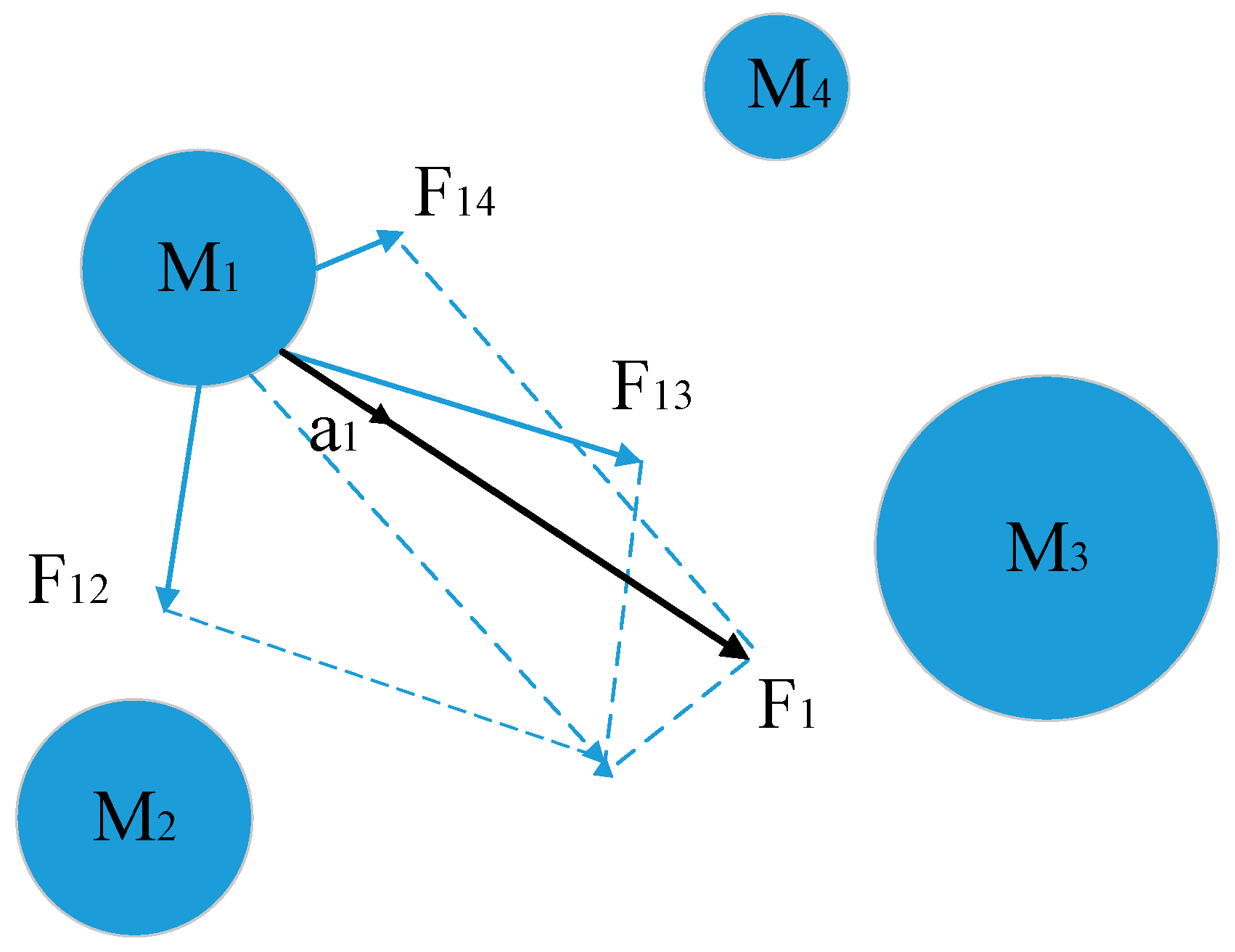
3.2.2. Gravitational Search Algorithm

GSA (gravitational search algorithm) is a new swarm intelligence optimization algorithm proposed, and the Schematic diagram of the GSA algorithm is shown as Figure 2.

In Figure 2, M₁, M₂, M₃, and M₄ represent four objects with different masses. The larger the area, the greater the mass. Object M₁ is subject to gravity F₁₂, F₁₃, and F₁₄ of object M₂, M₃, and M₄, respectively, producing a reasonable F₁ and corresponding acceleration a₁. Under the action of the resultant F, Object M₁ moves towards an F₁ direction. It can be seen from the figure that F₁ direction and F₁₃ direction are close to each other. In the figure, object M₃ has the maximum mass. Under the action of the surrounding gravity, object M₁ will approach the object with the maximum mass nearby. This approach is actually the optimization process of the gravity search algorithm. Therefore, the optimization process of the GSA algorithm is actually the process of finding the individual with the largest mass, and the quality of the optimization result is judged by the size of the individual mass.

Assuming a population of N particles $X_i$, in D-dimensional search space, defining the position and velocity of the first particle are $X_i=\left(X_i^1,X_i^2,\cdots ,X_i^k,\cdots X_i^D\right)$ and $V_i=\left(v_i^1,v_i^2,\cdots ,v_i^k,\cdots v_i^D\right)$, $i=1,2,\cdots ,N$, respectively, where $X_i^k$ and $v_i^k$ represent the position and velocity components of the particle i on the k-dimension, respectively. Then the mass and gravity of each particle are determined through evaluating the objective function values of each particle, calculating the acceleration and updating the speed and position on this basis.

Firstly, population initialization is carried out, including the initialization of position, velocity, acceleration, and mass of particles. Then, the mass of each particle is calculated. When carrying out the t-th iteration, the inertia mass $M_i\left(t\right)$ of particle i can be updated according to its fitness value. The updated formula is as follows:

$$mas{s}_i\left(t\right)\{\begin{array}{cc}\frac{fi{t}_i\left(t\right)-worst\left(t\right)}{best\left(t\right)-worst\left(t\right)}& if best\left(t\right)\ne worst\left(t\right)\\ 1& otherwise\end{array}$$

(10)

$$M_i\left(t\right)=\frac{mas{s}_i\left(t\right)}{{\displaystyle \sum _{j=1}^{N}mas{s}_j\left(t\right)}}$$

(11)

where $fi{t}_i\left(t\right)$ denotes the fitness of particle i at iteration t-th, $i=1,2,\cdots ,N$. For solving the minimum optimization problem, the optimal fitness $best\left(t\right)$ and the $worst\left(t\right)$ fitness word are expressed as follows:

$$best\left(t\right)=\underset{j\in \left\{1,2,\cdots ,N\right\}}{\min }fi{t}_j\left(t\right)$$

(12)

$$worst\left(t\right)=\underset{j\in \left\{1,2,\cdots ,N\right\}}{\max }fi{t}_j\left(t\right)$$

(13)

Conversely, it can be applied to the maximum optimization problem.

Then, calculating the gravity of each particle, when carrying out the t-th iteration, the mutual attraction of particle i and particle j in K-dimension is defined as:

$$F_{ij}^d\left(t\right)=G\left(t\right)\frac{M_i\left(t\right)\times M_j\left(t\right)}{R_{ij}\left(t\right)+\epsilon }\left(x_j^k\left(t\right)-x_i^k\left(t\right)\right)$$

(14)

where $M_j$ and $M_i$ represent the inertia mass of particle i and j, respectively. $\epsilon$ is constant. $G\left(t\right)$ denotes the gravitation coefficient for t-th iterations. $R_{ij}\left(t\right)$ denotes the distance between particle i and particle j (generally taking the Euclidean distance), shown as follows:

$$G\left(t\right)=G_0{e}^{-\alpha \frac{1}{T}}$$

(15)

$$R_{ij}\left(t\right)={\Vert X_i\left(t\right),X_j\left(t\right)\Vert }_2$$

(16)

where $G_0$ represents the universal gravitational constant of the universe at its earliest moments. $\alpha$ denotes the attenuation factor of the gravitational coefficient and is generally taken as a constant, and T represents the maximum number of iterations.

In GSA, the total force acting on the t-th iteration particle i in the K-dimension can be expressed as:

$$F_i^k\left(t\right)={\displaystyle \sum _{j=1,j\ne i}^{Kbest}ran{d}_i}\times F_{ij}^k\left(t\right)$$

(17)

where $ran{d}_i$ denotes a random number of $\left[0,1\right]$. The initial value of Kbest is N, which gradually decreases to 1 over time. It is defined as:

$$Kbest\left(t\right)=final\_per+\left(\frac{1-t}{T}\right)\times \left(100-final\_per\right)$$

(18)

Among them, $final\_per$ represents the percentage of particles that exert forces on other particles.

Finally, the particles’ position movement is calculated. According to Newton’s second law, when the t-th iteration is performed, the acceleration of particle i on the K- dimension can be defined as:

$$a_i^k\left(t\right)=\frac{F_i^k\left(t\right)}{M_i\left(t\right)}$$

(19)

In each iteration of the GSA, the particle updates the velocity v and position x of particle i according to the following formula:

$$v_i^k\left(t+1\right)=ran{d}_j\times v_i^k\left(t\right)+a_i^k\left(t\right)$$

(20)

$$x_i^k\left(t+1\right)=x_i^k\left(t\right)+v_i^k\left(t+1\right)$$

(21)

3.2.3. Improved Gravitational Search Algorithm

When predicting via SVM, the different choices of penalty parameter C and kernel parameter g in the Gauss kernel function have a great impact on the prediction accuracy. In order to avoid falling into the local optimum when the gravitational search algorithm optimizes the parameters of the support vector machine, the improved gravitational search algorithm (IGSA) in this paper was constructed by introducing the memory function and boundary mutation strategy of PSO (particle swarm optimization), shown as follows:

1. Introducing the memory function of PSO. When updating particles, GSA only considers the influence of the current position of particles but does not take the memory of particles into account. Therefore, the global memory function of particle swarm optimization was introduced in this paper. GSA is embedded in the memory function, that is to say, the idea of the best position that the whole population has searched so far was added to the velocity update equation, so as to improve the local development ability of GSA:

$$v_i^k\left(t+1\right)=ran{d}_j\times v_i^k\left(t\right)+a_i^k\left(t\right)+c_1\times ran{d}_i\times \left(gbest-x_i^k\left(t\right)\right)$$

(22)

where $c_1$ is learning factor and C means the best location the whole group has found so far.

2. Introducing the boundary mutation strategy of PSO. In the process of GSA iteration, under the action of the law of gravitation and Newton’s second law, if the particle’s position exceeds the set range $\left[x_{\min },x_{\max }\right]$, the standard GSA will force the particle to return to the boundary. If the particle gathers too much on the boundary of the feasible region, it is not conducive to the convergence of GSA. In order to improve the convergence of GSA, the boundary mutation strategy is introduced as follows:

$$\begin{array}{l}if x_i<x_{\min } or x_i>x_{\max }\\ then x_i=\mathrm{rand}\times \left(x_{\max }-x_{\min }\right)+x_{\min }\end{array}$$

(23)

After the boundary mutation, the particles do not gather on the boundary, which increases the diversity of the population and helps the algorithm to find the optimal solution faster.

3.2.4. IGSA–SVM Forecasting Model

The improved IGSA was used to optimize the parameters of SVM to ensure good prediction results. The specific steps are as follows.

Step 1 Initialization of parameter. Setting N as population size, $x_i^k$, and $v_i^k$ represents position and velocity of N particles, respectively. Then determining the number of iterations t, the learning factor $c_1$, and the range of parameters C and g.

Step 2 Calculating the fitness of the particle and finding out the optimal solution Kbest and the position $gbest$ of the optimal particle.

Step 3 Updating the inertial mass $M_i\left(t\right)$ of particles by Equations (10)–(13), the gravitational constant $G\left(t\right)$ by Equation (15), and calculating Euclidean distance $R_{ij}\left(t\right)$ among particles by Equation (16).

Step 4 Calculating the sum of forces $F_i^k\left(t\right)$ in each direction of the particle by Equation (17), and the acceleration of the particle according to Equation (19).

Step 5 Updating the position and velocity of particles by Equations (20)–(22).

Step 6 Judging whether the boundary conditions are satisfied by Equation (23).

Step 7 Return to step 2 and iterate until the maximum number of iterations or accuracy requirements are met, and output (C, g).

Step 8 The IGSA is used to optimize the parameter values of SVM, and the forecasting model is obtained.

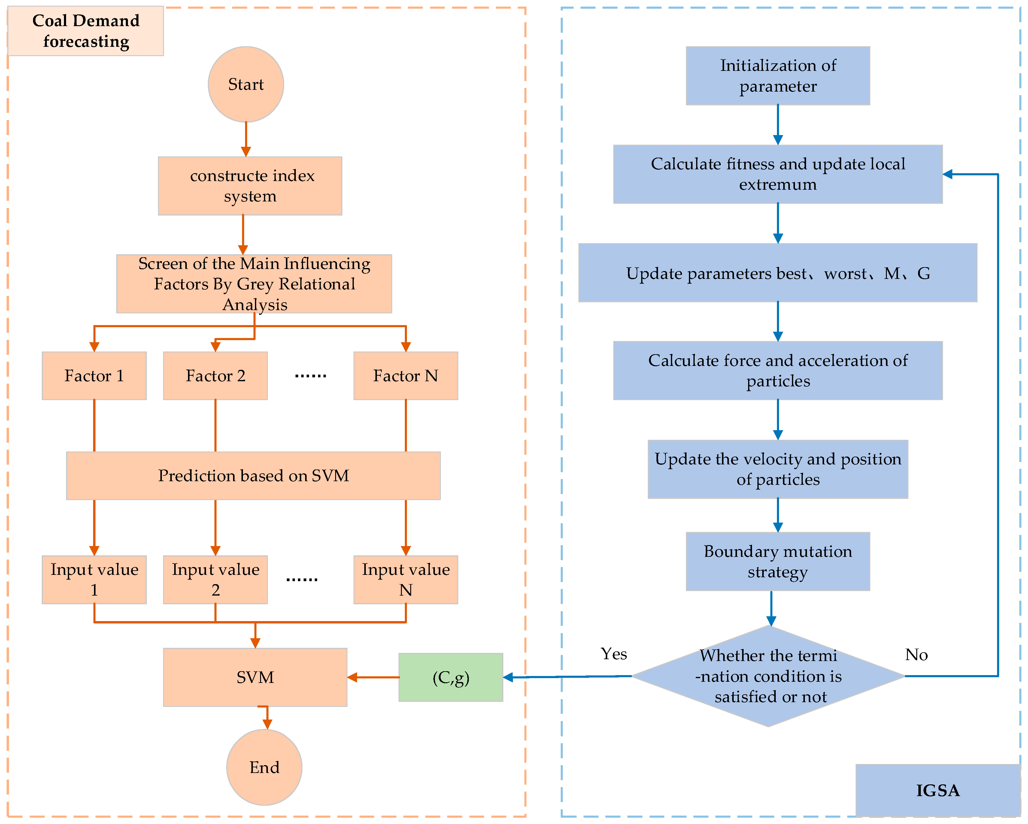
3.3. Forecasting Process

According to the previous analysis, coal demand forecasting is affected by many factors. In order to predict coal demand scientifically and accurately, firstly, sample data of 15 influencing factors were collected. Then, according to the grey relational analysis method, the main influencing factors of coal demand were selected and used as the input value of the IGSA–SVM model. On that basis, according to the steps 1–8 above, forecasting the coal demand was based on IGSA–SVM. Repeat the above steps until the number of iterations is reached. Finally, the IGSA–SVM forecasting model was obtained to forecast the coal demand. The prediction process is shown in Figure 3.

4. Empirical and Comparative Analysis

In this section, influencing factor screening for model input was determined first. Then the effectiveness of IGSA–SVM in predicting coal demand was further proven by comparing the errors of BP, SVM, and GSA–SVM. Through empirical and comparative analysis, the IGSA–SVM was used to forecast China’s coal demand in 2018–2024.

4.1. Influencing Factor Screening for Model Input

According to the influence factors selected in Figure 1, this paper selected the relevant data, that is, GDP, total population, CPI, value added of secondary industry, urbanization rate, energy consumption intensity, the proportion of coal consumption to energy consumption, coal reserves, inventory of coal and products, quantity of imported coal, average annual price of Shanxi premium blended coal in Qinhuangdao Port, new productivity increased in raw coal mining, national railway coal freight volume, completion of investment in industrial pollution control, and sulfur dioxide emissions, from 1990 to 2017 as the research object. Among them, in addition to the average annual price of Shanxi premium blended coal in Qinhuangdao Port and new productivity increased in raw coal mining indicators’ data from the China coal industry association, the other indicators’ data came from the relevant data issued by the National Bureau of Statistics and the Statistical Yearbook.

In order to determine the input index of the prediction model, the grey correlation analysis was used to analyze the correlation degree between influencing factors and coal demand, as shown in

Table 1. The calculation results of the grey relational degrees for influencing factors.

Influencing Factor	Grey Relational Degree
GDP	0.8602
Total Population	0.943
CPI	0.9754
Value added of secondary industry	0.9517
Urbanization rate	0.9733
Energy consumption intensity	0.8982
The proportion of coal consumption to energy consumption	0.9573
Coal reserves	0.9241
Inventory of Coal and Products	0.65
Quantity of imported coal	0.6263
Average annual price of Shanxi premium blended coal in Qinhuangdao Port	0.9426
New Productivity Increased in Raw Coal Mining	0.9364
National Railway Coal Freight Volume	0.9861
Completion of Investment in Industrial Pollution Control	0.9544
Sulfur dioxide emissions	0.9285

.

The six factors whose grey relational degree was greater than 0.95 were selected as the coal consumption forecasting model input. They are CPI, value added of secondary industry, urbanization rate, the proportion of coal consumption to energy consumption, national railway coal freight volume, and completion of investment in industrial pollution control. The model output is the power grid investment, as shown in

Table 2. Data of the main influencing factors.

Year	Total Coal Consumption (Ten Thousand Tons of Standard Coal)	CPI (1978 = 100)	Value Added of Secondary Industry (%)	Urbanization Rate (%)	The Proportion of Coal Consumption to Energy Consumption (%)	National Railway Coal Freight Volume (Ten Thousand Yuan)	Completion of Investment in Industrial Pollution Control (Ten Thousand Yuan)
1990	75211.686	216.4	41	26.41	76.2	62870	454465
1991	78978.863	223.8	41.5	26.37	76.1	62603	597306
1992	82641.69	238.1	43.1	27.63	75.7	64108	646661
1993	86646.771	273.1	46.2	28.14	74.7	65336	693270
1994	92052.75	339	46.2	28.62	75	65943	833313
1995	97857.296	396.9	46.8	29.04	74.6	67357	987376
1996	103794.16	429.9	47.1	29.37	74.7	72058	956135
1997	98793.695	441.9	47.1	29.92	71.5	70345	1164386
1998	92020.944	438.4	45.8	30.4	69.6	64081	1220461
1999	81862	432.2	45.4	38.89	67.1	64917	1527307
2000	100670.34	434	45.50	36.00	69.00	68545	2347895
2001	105771.96	437	44.80	38.00	68.00	76625	1745280
2002	116160.25	433.5	44.50	39.00	69.00	81852	1883663
2003	138352.27	438.7	45.60	41.00	70.00	88132	2218281
2004	161657.26	455.8	45.90	42.00	70.00	99210	3081060
2005	189231.16	464	47.00	43.00	72.00	107082	4581909
2006	207402.11	471	47.60	44.00	72.00	112034	4839485
2007	225795.45	493.6	46.90	46.00	73.00	122080.63	5523909
2008	229236.87	522.7	47.00	47.00	72.00	134325	5426404
2009	240666.22	519	46.00	48.00	72.00	132720.15	4426207
2010	249568.42	536.1	46.50	50.00	69.00	156020	3969768
2011	271704.19	565	46.50	51.00	70.00	172125.74	4443610
2012	275464.53	579.7	45.40	53.00	69.00	168515.29	5004573
2013	280999.36	594.8	44.20	54.00	67.00	167945.66	8496647
2014	279328.74	606.7	43.30	55.00	66.00	164130.57	9976511
2015	273849.49	615.2	41.10	56.00	64.00	143221.23	7736822
2016	270320	627.5	40.10	57.00	62.00	131790.73	8190041
2017	278159	637.5	40.50	59.00	60.40	149129.86	6815345

Data sources: Statistical Yearbook 1990–2016 and official website of national bureau of statistics (http://www.stats.gov.cn/).

.

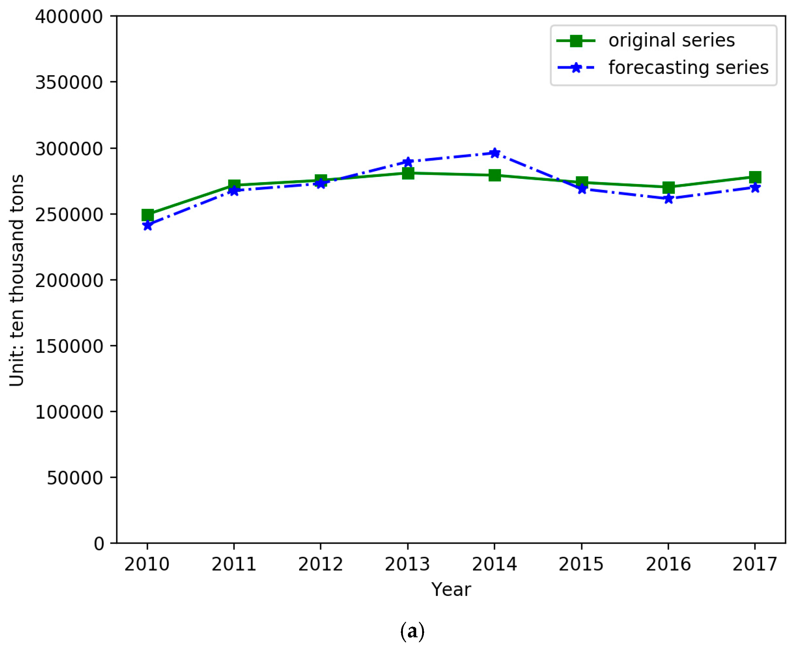
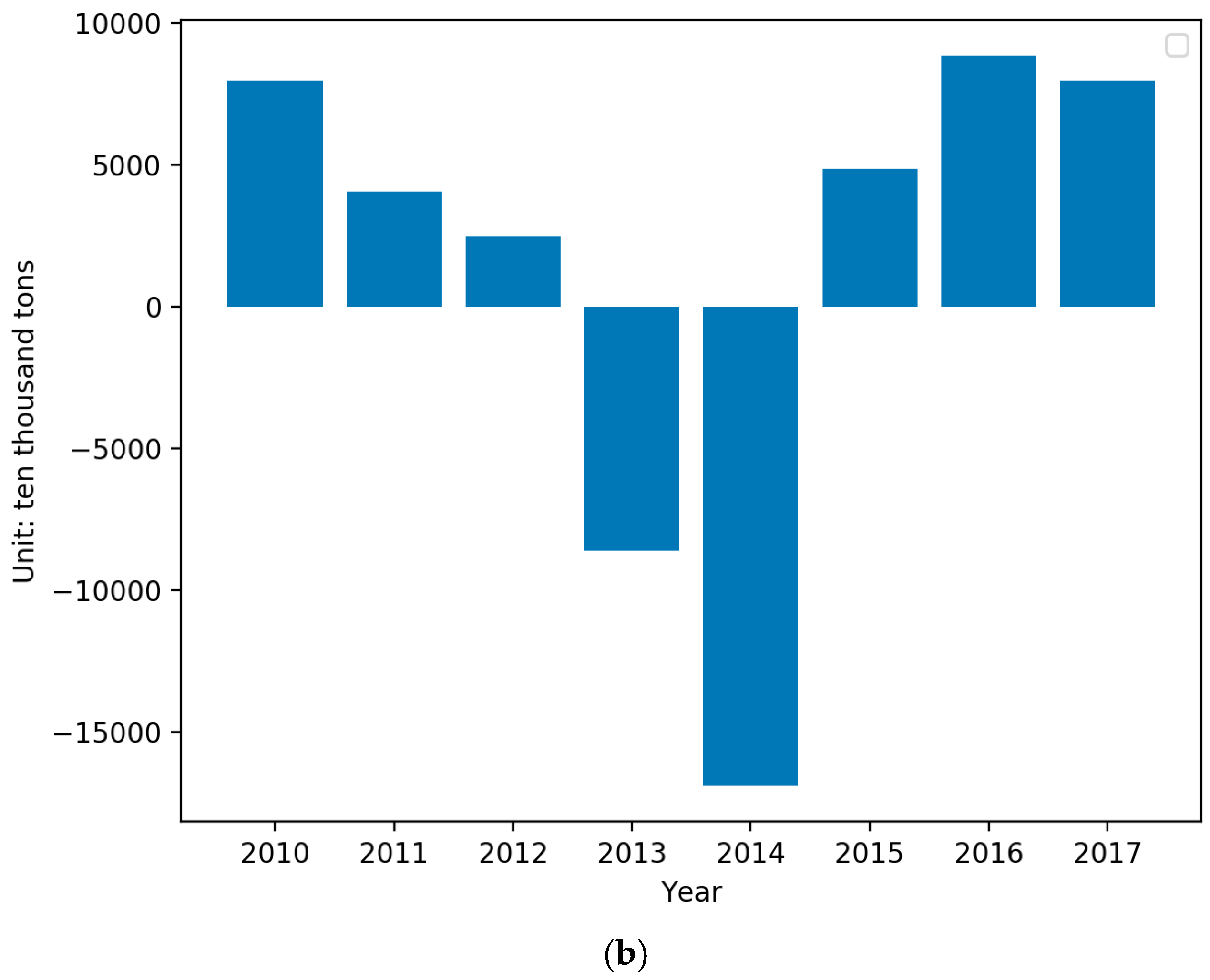
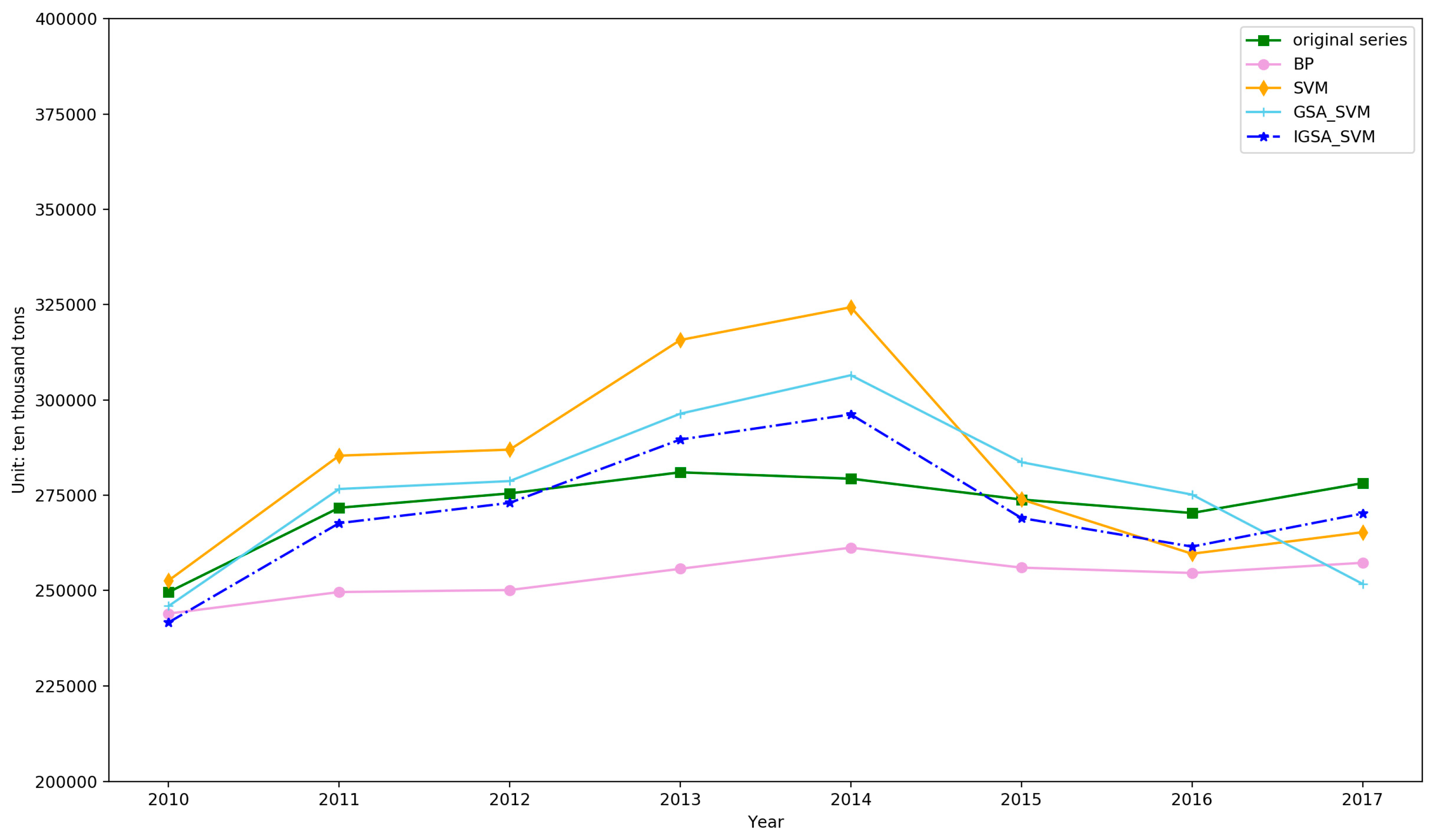
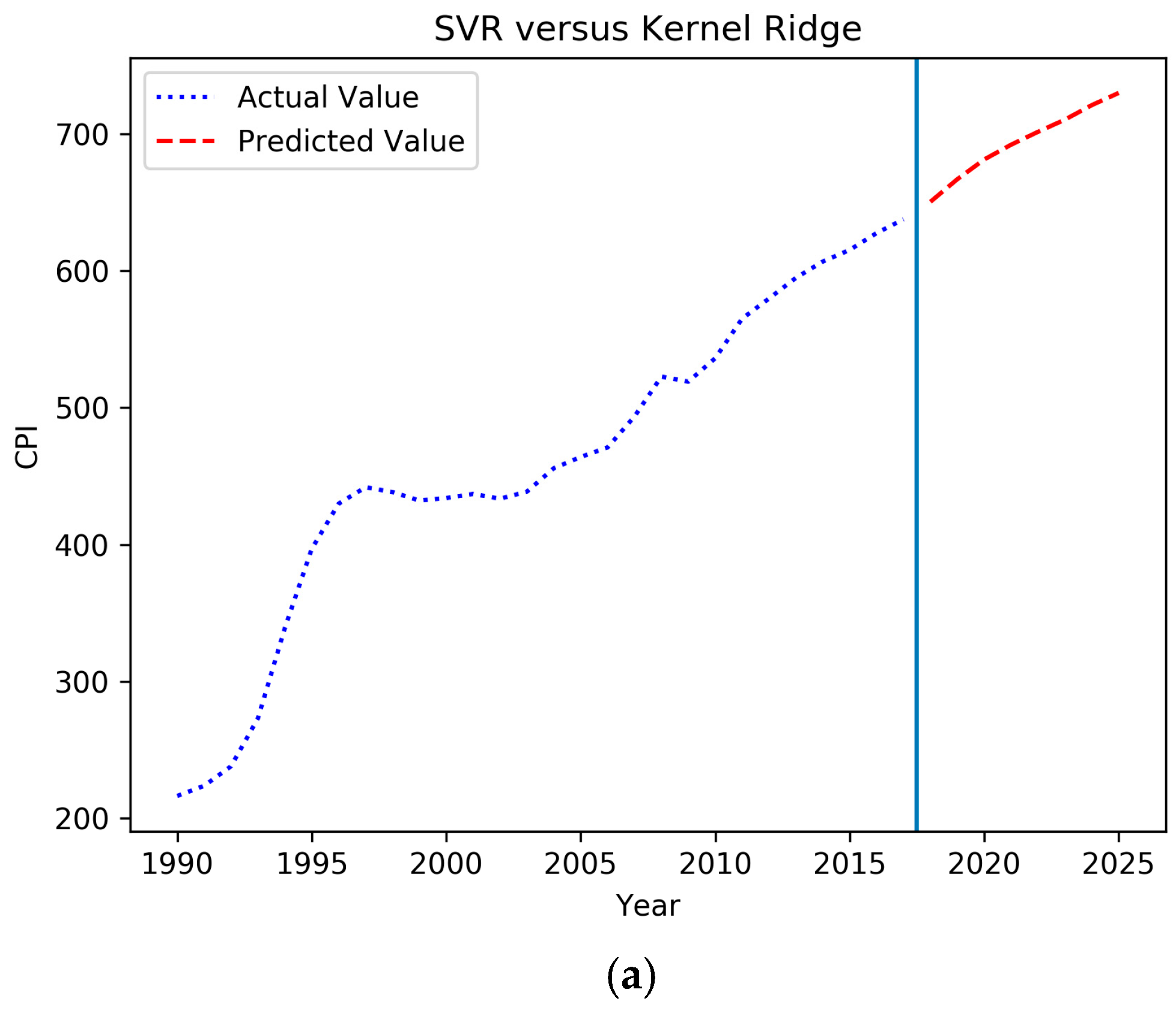
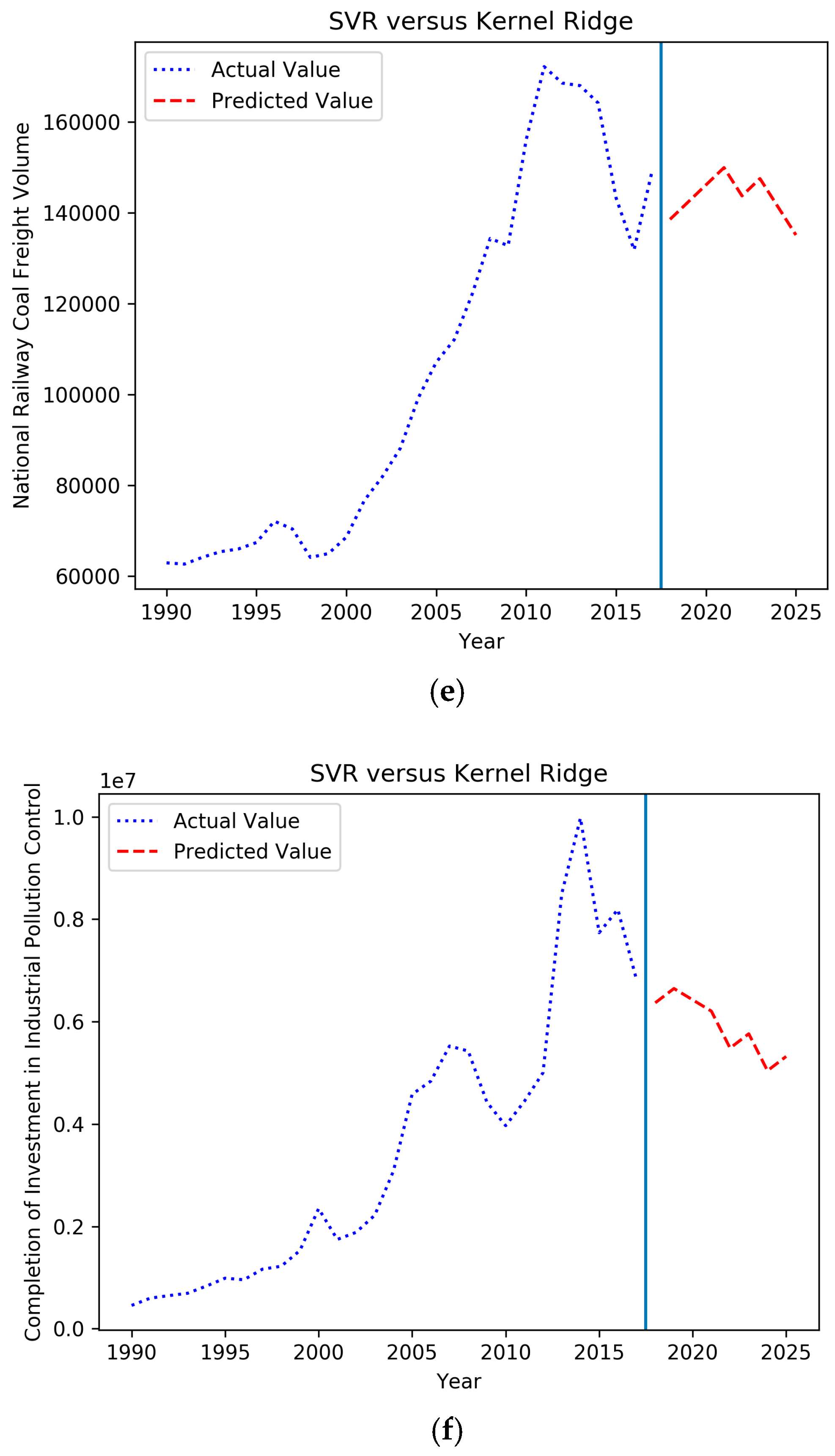
4.2. Forecasting and Comparative Analysis

Taking 1990–2009 as the training set and 2010–2017 data as the test set to forecast, the model parameters settings are as follows: population size N = 20, maximum number of iterations MAX_IT = 100, the optimal range of penalty parameter C is [1,500], the optimum range of kernel parameter g is [0.001,200], G₀ = 100, α = 20, and c₁ = 2. The forecasting results and the residuals are shown in Figure 4.

According to Figure 3, it can be seen that IGSA–SVM has a good fitting effect on predicting coal consumption. Furthermore, the errors of IGSA–SVM, GSA–SVM, SVM, and BP in predicting coal demand in 2010–2017 were compared and analyzed, including RMSE (root mean square deviation), MAE (mean absolute error), and MAPE (mean absolute percent error). The comparison results are shown in

Table 3. Error analysis and comparison.

Error Types	BP	SVM	GSA–SVM	IGSA–SVM
RMSE	19798.56	21902.20	15164.49	8721.86
MAE	18877.36	16439.78	11925.47	7694.94
MAPE	6.87	5.94	4.31	2.82

below.

From the comparative analysis of the errors in Table 3, it can be seen that the IGSA–SVM prediction has the smallest errors among the four models. The values of RMSE, MAE, and MAPE are 8721.86, 7694.94, and 2.82%, respectively. Then, there are the GSA–SVM and SVM prediction models. The BP model has the worst prediction effect, and the MAPE reached 6.87%. The main reason is that BP prediction needs more historical data for training.

From the comparison of the predictions in Figure 5, it can be seen that the IGSA–SVM forecasting model fits well with the real data when predicting coal consumption. Combining Table 3 and Figure 5, it can be concluded that the order of prediction accuracy of the four prediction models is IGSA–SVM > GSA–SVM > SVM > BP. Therefore, we chose IGSA–SVM to forecast China’s coal consumption.

4.3. Forecasting Based on the IGSA–SVM

According to the data of six key factors from 1990 to 2017, the data of six factors from 2018 to 2025 were predicted by SVM, as shown in Figure 6, as input variables of the IGSA–SVM forecasting model, and the forecasted results are shown in Figure 7.

As we can see from Figure 6, combined with the change trend of six key factors affecting coal demand selected in this paper, the following findings are made. CPI is on a slight upward trend. Value added of secondary industry is on a slight downward trend. Urbanization rate is on a slight upward trend. The proportion of coal consumption to energy consumption is on a steady downward trend. Finally, the national railway coal freight volume fluctuates between increase and decrease. Completion of investment in industrial pollution control shows a downward trend.

Affected by these factors, as we can see from Figure 7, coal consumption grew slowly in 2018 to 2025, peaked in 2019, and began to decline gradually. According to the predicted results, combined with the impact of the factors, value added of secondary industry, the proportion of coal consumption to energy consumption, and completion of investment in industrial pollution control are the key factors leading to the turning point of demand. This means that the decline in coal demand is related to policy constraints, such as the increase of the proportion of tertiary industry output and the reduction of the proportion of coal consumption, as well as the gradual saturation of industrial pollution control projects. If we want to further reduce the demand for coal in China, energy efficiency must be comprehensive, and the coal-based energy consumption structure needs further optimization. In terms of future energy development, we must be committed to adjusting the structure of the energy industry, developing new energy sources, improving the level of re-electrification, and realizing clean substitution and electric energy substitution.

The forecasting results are in line with the development trend of the energy revolution, especially the peak value forecasting results, and are helpful to energy strategic planning, overall planning of coal production and consumption, and ensuring the healthy and coordinated development of the coal industry. According to the prediction results of the model, the base line of coal safety supply in each year is calculated according to the coefficient of raw coal converted into standard coal. In addition, the coal production capacity can be controlled at this bottom line, providing an important reference value for the reduction of production capacity.

5. Conclusions

In order to predict China’s coal demand more accurately, firstly, we selected 15 influence factors that affect coal consumption from the four dimensions of economy, energy, coal industry, and environmental constraints, and the grey correlation analysis method was used to select six key influence factors as input variables of the IGSA–SVM prediction model. Then, PSO was used to improve the GSA, which is used to optimize the kernel function of SVM, and the IGSA–SVM algorithm was obtained. Next, the data from 1990 to 2009 were selected as the training set, and the data from 2010 to 2017 were used as the test set. The errors of BP, SVM, GSA–SVM, and IGSA–SVM in prediction were compared, which further proved the effectiveness of IGSA–SVM in coal demand prediction.

Finally, the IGSA–SVM was used to forecast China’s coal demand in 2018–2025. According to the forecasting results, it can be seen that China’s coal consumption from 2018 to 2025 will have a trend from growth to decrease. According to the forecasting results, it will be better to have an active response for the government and industry, enacting the relevant policies, further optimizing the structure of the coal industry, transforming and upgrading it and eliminating backward production capacity, improving the efficiency of coal utilization, establishing an effective modern supervision system of coal, solving the excess capacity, and promoting a healthy development of the coal industry through speeding up clean technology innovation and development.

In the future, the application scope of IGSA–SVM can be further expanded, and the coal demand of different industries and provinces can be predicted. This is of great significance to the transformation and development of high energy-consuming industries and coal resource-based provinces and to adapt to the energy revolution.

References

1. Shi, D. Current situation and development Suggestions of coal chemical industry. Guangzhou Chem. Ind. 2018, 24, 14–16. [Google Scholar]
2. Michieka, N.M.; Fletcher, J. An investigation of the role of China’s urban population on coal consumption. Enery Policy 2012, 48, 668–676. [Google Scholar] [CrossRef]
3. Chong, C.; Ma, L.; Li, Z.; Ni, W.; Song, S. Logarithmic mean Divisia index (LMDI) decomposition of coal consumption in China based on the energy allocation diagram of coal flows. Energy 2015, 85, 366–378. [Google Scholar] [CrossRef]
4. Kulshreshtha, M.; Parikh, J.K. Modeling demand for coal in India: Vector autoregressive models with ciontegrated variables. Energy 2000, 25, 149–168. [Google Scholar] [CrossRef]
5. Lin, B.; Wu, W. Coal demand in China’s current economic development. China Soc. Sci. 2018, 2, 141–161. [Google Scholar]
6. Jebaraj, S.; Iniyan, S.; Goic, R. Forecasting of Coal Consumption Using an Artificial Neural Network and Comparison with Various Forecasting Techniques. Energy Sources Part. A Recovery Utilization Environ. Eff. 2011, 33, 1305–1316. [Google Scholar] [CrossRef]
7. Zhu, Q.; Zhang, Z.; Chai, J.; Wang, S. Coal demand forecasting model based on consumption structure division. Syst. Eng. 2014, 32, 112–123. (In Chinese) [Google Scholar]
8. Hao, Y.; Zhang, Z.Y.; Liao, H.; Wei, Y.M. China’s farewell to coal: A forecast of coal consumption through 2020. Energy Policy 2015, 86, 444–455. [Google Scholar] [CrossRef]
9. Yawei, O.; Li, O. A forecast of coal demand based on the simultaneous equations model. In Proceedings of the 2011 IEEE International Symposium on IT in Medicine and Education, Cuangzhou, China, 9–11 December 2012. [Google Scholar]
10. Wang, Y.; Li, X. The influence of renewable energy power generation development on coal demand. J. North. China Electr. Power Univ. (Soc. Sci. Ed.) 2014, 5, 13–16. [Google Scholar]
11. Wang, Y.; Chen, X.; Han, Y. Forecast of Passenger and Freight Traffic Volume based on Elasticity Coefficient Method and Grey Model. Proced. Soc. Behav. Sci. 2013, 96, 136–147. [Google Scholar] [CrossRef] [Green Version]
12. Xiong, Y.; Zou, J.; Liu, L. Energy profile model based on multiple linear regression analysis. China High.-tech Zone 2018, 13, 52. [Google Scholar]
13. Tsekouras, G.J.; Dialynas, E.N.; Hatziargyriou, N.D. A non-linear multivariable regression model for midterm energy forecasting of power systems. Electr. Power Syst. Res. 2007, 77, 1560–1568. [Google Scholar] [CrossRef]
14. Huang, Y.; Zhao, G.; Wang, Y. Research on China’s energy consumption combination forecasting model based on Shapley value. Energy Eng. 2012, 6, 5–9. [Google Scholar]
15. Chi, K.C.; Nuttall, W.J.; Reiner, D.M. Dynamics of the UK natural gas industry: System dynamics modelling and long-term energy policy analysis. Technol. Forecast. Soc. Chang. 2009, 76, 339–357. [Google Scholar] [Green Version]
16. Kou, A.; Zhou, W.; Hu, Q. GM (1,1) Model for Forecasting and Analysis of China’s Energy Consumption. China Market. 2018, 16, 15–16. [Google Scholar]
17. Zhang, J.; Yao, Z.; Xu, X.; Nan, Y. Coal demand forecasting based on Grey GM (1,1) model. J. North. China Inst. Sci. Technol. 2016, 13, 106–108. (In Chinese) [Google Scholar]
18. Khotanzad, A.; Afkhami-Rohani, R.; Maratukulam, D. ANNSTLF-artificial neural network short-term load forecaster-generation three. IEEE Trans. Power Syst. 1998, 13, 1413–1422. [Google Scholar] [CrossRef]
19. De, G.; Gao, W. Forecasting China’s Natural Gas Consumption Based on AdaBoost-Particle Swarm Optimization-Extreme Learning Machine Integrated Learning Method. Energies 2018, 11, 2938. [Google Scholar] [CrossRef]
20. Xie, M.; Deng, J.; Liang, J. Cooling load forecasting method based on support vector machine optimized with entropy and variable accuracy roughness set. Power Syst. Technol. 2017, 41, 210–214. [Google Scholar]
21. Dai, S.; Niu, D.; Han, Y. Forecasting of Energy-Related CO2 Emissions in China Based on GM (1,1) and Least Squares Support Vector Machine Optimized by Modified Shuffled Frog Leaping Algorithm for Sustainability. Sustainability 2018, 10, 958. [Google Scholar] [CrossRef]
22. Damrongkulkamjorn, P.; Churueang, P. Monthly energy forecasting using decomposition method with application of seasonal ARIMA. In Proceedings of the 2005 International Power Engineering Conference, Singapore, 29 November–2 December 2005. [Google Scholar]
23. Li, T.; Hu, Z.; Jia, Y.; Wu, J.; Zhou, Y. Forecasting Crude Oil Prices Using Ensemble Empirical Mode Decomposition and Sparse Bayesian Learning. Energies 2018, 11, 1882. [Google Scholar] [CrossRef]
24. Liu, X.; Mao, G.; Ren, J.; Li, R.Y.M.; Guo, J.; Zhang, L. How might China achieve its 2020 emissions target? A scenario analysis of energy consumption and CO2 emissions using the system dynamics model. J. Clean. Prod. 2015, 103, 401–410. [Google Scholar] [CrossRef]
25. Mollaiy-Berneti, S. Developing energy forecasting model using hybrid artificial intelligence method. J. Cent. South. Univ. Engl. Ed. 2015, 22, 3026–3032. [Google Scholar] [CrossRef]
26. Cao, G.; Wu, L. Support vector regression with fruit fly optimization algorithm for seasonal electricity consumption forecasting. Energy 2016, 115, 734–745. [Google Scholar] [CrossRef]
27. Kuo, P.-H.; Huang, C.-J. A High Precision Artificial Neural Networks Model for Short-Term Energy Load Forecasting. Energies 2018, 11, 213. [Google Scholar] [CrossRef]
28. Zhang, M.; Mu, H.; Li, G.; Ning, Y. Forecasting the transport energy demand based on PLSR method in China. Energy 2009, 34, 1396–1400. [Google Scholar] [CrossRef]
29. Hsu, J.F.; Chang, J.M.; Cho, M.Y.; Wu, Y.H. Development of Regression Models for Prediction of Electricity by Considering Prosperity and Climate. In Proceedings of the 2016 3rd International Conference on Green Technology and Sustainable Development (GTSD), Kaohsiung, Taiwan, 24–25 November 2016. [Google Scholar]
30. Hu, Y.C. A genetic-algorithm-based remnant grey prediction model for energy demand forecasting. PLoS ONE 2017, 12, e0185478. [Google Scholar] [CrossRef]
31. Zou, S.; Ding, Z. China’s coal demand forecasting model based on ABA-ESA. China Coal 2018, 44, 9–14. [Google Scholar]
32. Kefayat, M.; Ara, A.L.; Niaki, S.A.N. A hybrid of ant colony optimization and artificial bee colony algorithm for probabilistic optimal placement and sizing of distributed energy resources. Energy Convers. Manag. 2015, 92, 149–161. [Google Scholar] [CrossRef]
33. Rahman, M.N.; Esmailipour, A.; Zhao, J. Machine Learning with Big Data An Efficient Electricity Generation Forecasting System. Big Data Res. 2016, 5, 9–15. [Google Scholar] [CrossRef]
34. Wang, R.; Li, J.; Wang, J.; Gao, C. Research and Application of a Hybrid Wind Energy Forecasting System Based on Data Processing and an Optimized Extreme Learning Machine. Energies 2018, 11, 1712. [Google Scholar] [CrossRef]
35. Dai, S.; Niu, D.; Li, Y. Forecasting of Energy Consumption in China Based on Ensemble Empirical Mode Decomposition and Least Squares Support Vector Machine Optimized by Improved Shuffled Frog Leaping Algorithm. Appl. Sci. 2018, 8, 678. [Google Scholar] [CrossRef]
36. Zhang, L.; Ge, R.; Chai, J. Prediction of China’s Energy Consumption Based on Robust Principal Component Analysis and PSO-LSSVM Optimized by the Tabu Search Algorithm. Energies 2019, 12, 196. [Google Scholar] [CrossRef]
37. Han, Z.; Wan, J.; Liu, K. Prediction and model optimization of gasoline octane number based on near-infrared spectroscopy. Anal. Lab. 2015, 34, 1268–1271. [Google Scholar]
38. Liu, A.; Xue, Y.; Hu, J.; Liu, L. Super-short-term prediction of wind power based on GA optimization SVM. Power Syst. Prot. Control. 2015, 2, 90–95. (In Chinese) [Google Scholar]
39. Saini, L.M.; Aggarwal, S.K.; Kumar, A. Parameter optimisation using genetic algorithm for support vector machine-based price-forecasting model in National electricity market. IET Gener. Trans. Distrib. 2010, 4, 36–49. [Google Scholar] [CrossRef]
40. Zhu, C.; Chen, X.; Wang, Z.; Zhang, X. Defect prediction model for object oriented software based on particle swarm optimized SVM. Comput. Appl. 2017, 37, 60–64. [Google Scholar]
41. Bao, L.; Chen, H.; Guo, J.; Yuan, Y. Application of SVM based on improved PSO algorithm in methane measurement. Chin. J. Sens. Actuators. 2017, 9, 1454–1458. (In Chinese) [Google Scholar] [CrossRef]
42. Rubio, G.; Pomares, H.; Rojas, I.; Herrera, L.J. A heuristic method for parameter selection in LS-SVM: Application to time series prediction. Int. J. Forecast. 2010, 3, 725–739. [Google Scholar] [CrossRef]
43. Xu, D.; Ding, S. Research on improved GWO-optimized SVM-based short-term load prediction for cloud computing. Computer Engineering and Applications. Comput. Eng. Appl. 2017, 7, 68–73. (In Chinese) [Google Scholar]
44. Feng, T.; Zhong, Y.; Liu, X.; Yu, L. Application of least square support vector machine based on adaptive artificial swarm optimization algorithm in deformation prediction. J. Jiangxi Univ. Sci. Technol. 2008, 39, 35–39. [Google Scholar]
45. Rashedi, E.; Nezamabadi-pour, H.; Saryazdi, S. GSA: A Gravitational Search Algorithm. Inf. Sci. 2009, 179, 2232–2248. [Google Scholar] [CrossRef]
46. Wang, H.; Han, Z.; Xu, X.; Li, X. Prediction model of steam turbine exhaust enthalpy based on gray correlation analysis and gsa-lssvm. Electr. Power Constr. 2016, 37, 115–122. (In Chinese) [Google Scholar]
47. Chen, Y.; Yin, X.; Tan, R. A network security situation prediction model based on gsa-svm. J. Air Force Eng. Univ. (Nat. Sci. Ed.) 2018, 19, 82–87. [Google Scholar]
48. Cui, D.; Huang, E. Application of improved gravity search algorithm and support vector machine in monthly runoff prediction in dry season. People’s Pearl River 2016, 37, 48–52. [Google Scholar]
49. Deng, J. Grey Theory Foundation; Huazhong University of Science and Technology Press: Wuhan, China, 2002. [Google Scholar]
50. Mei, H.; Liu, D.; He, Y. Fault Diagnosis of SVM Analog Circuits Optimized by Improved Gravity Search Algorithms. Microelectr. Comput. 2018, 408, 115–121. [Google Scholar]
Figure 1. Influence factors system for coal demand forecasting.
Energies 12 02249 g001
Figure 2. The schematic diagram of the gravitational search algorithm (GSA).
Energies 12 02249 g002
Figure 3. The flow chart of forecasting.
Energies 12 02249 g003
Figure 4. The prediction and residual figures by IGSA–SVM. (a) The prediction figure; (b) the residual figure.
Energies 12 02249 g004aEnergies 12 02249 g004b
Figure 5. Forecasting results comparison.
Energies 12 02249 g005
Figure 6. Coal consumption key influencing factors prediction curve. (a) Forecasting of consumer price index (CPI); (b) forecasting of value added of secondary industry; (c) forecasting of urbanization rate; (d) forecasting of the proportion of coal consumption to energy consumption; (e) forecasting of national railway coal freight volume; (f) forecasting of completion of investment in industrial pollution control.
Energies 12 02249 g006aEnergies 12 02249 g006bEnergies 12 02249 g006c
Figure 7. The forecasting results of coal consumption from 2018 to 2025 in China.
Energies 12 02249 g007