A High Performance Optimizing Method for Modeling Photovoltaic Cells and Modules Array Based on Discrete Symbiosis Organism Search

Abstract

Exact models are a necessary prerequisite for optimal hardware configuration and the design of high-performance controllers. The photovoltaic system is considered a dynamic nonlinear multimodal system, where an optimization method must be used to resolve non-linearity and to identify the parameters describing the models of such systems. This has incited several researchers to work on and to develop several optimization methods. Recently, a number of methods have been proposed, including deterministic approaches, as well as probabilistic and stochastic numerical approaches, that aimed at obtaining a more accurate model for the PV cell and module array. This paper demonstrates the application of a performance optimization method based on discrete symbiotic organism search (DSOS), that mimics the behaviors of an organism in an ecosystem to survive. The high performance of such a method is attributable to the simplicity of the algorithm used; this algorithm is different from other heuristic algorithms, in that the GA needs two tuning parameters, i.e., the cross over and mutation rate, while the harmony search needs three rules to adjust and improvise new harmony, being memory consideration, pitch adjustment, and random choosing. Meanwhile, in the ABC algorithm, three phases are introduced to find the best food source, that is, the employed bee, the onlooker bee, and the scout bee phases, while the DSOS algorithm did not need any tuning parameters, wherein the proposed algorithm was used in both a single diode and double diode model across three test cases in the study. Compared to other previously published works, the level of performance of the algorithm is high in both implementation and accuracy; the DSOS algorithm is more capable of reaching the best set of solutions. The Mann-Whitney-Wilcoxon test to evaluate the discrete solutions of the algorithm for multiple runs with a 5% degree of confidence was evaluated and performed with a good level of accuracy.

1. Introduction

The continuous integration of renewable energy resources and the increased use of the photovoltaic system to generate green and efficient energy have given researchers more opportunities to study the generation of green power. The goal has been to enhance the output from this energy source, as well as to enhance the efficiency of the panel.

Over the last two decades, several countries have sought the benefits that these sustainable resources can supply. Photovoltaic energy is ubiquitous in rural and urban areas. Due to their topography, previously inaccessible villages have now been electrified by photovoltaic systems. In Africa, where water resources are limited, people pump water using energy from photovoltaic systems. In addition, many telecommunications base stations that are far from urban areas, or that are located on mountains and along highways, are supplied by photovoltaic energy [1]. Therefore, by using cheap photovoltaic energy to power communications systems, for example, this may help to reduce the likelihood—or keep users informed—of a situation like a forest fire. That is why we have to focus on increasing the implementation of this kind of energy and to take advantage of the cell and the module array of the photovoltaic system.

The global efficiency of the photovoltaic system is achieved through accurate mathematical modeling from the solar cell to the panel.

In fact, the mathematic model for the smallest entity (the cell) of the photovoltaic generator is a multivariable nonlinear problem. Thus, it has to be accurately studied to fit the physical model, as well as the experimental measurements and results.

Over the last few years, several researchers have been interested in the optimization problem relating to the extraction of solar cell and module array parameters, bearing in mind that an accurate model can increase the output in terms of power generated by any photovoltaic system. This is interesting, because a diode ideality factor that is inaccurate by even 1% can result in approximately a 10% loss of power in the MPP.

Several methods and parameter extraction techniques based on the deterministic approach have been studied, whilst other methods based on the probabilistic, stochastic numerical approach have been used to develop an accurate model for the PV cell. However, it can be demonstrated that no single process can ensure a completely potent result for the parameter extraction problem.

Several methods have been used to get over the non-linearity of the optimization problem and to overcome the implicit form between the current and voltage that characterizes the mathematic model of the photovoltaic cell and module. Below is an overview of the literature associated with the problem of parameter optimization or estimation of the solar cell, as well as the status of current research.

The electrical parameters describing the electrical equivalent circuit operation of the cell differ from one model to the next. A PV array (or cell) is described by the generated current (I) versus the output voltage of the panel (V), and by the power (P) versus the voltage (V). Therefore, either the cell or the panels can be modeled as a DC current source [2].

In the literature, we find different mathematical models depending on the number of diodes in the model described. In most cases, researchers are interested in the single diode model (SDM) and the double diode model (DDM), illustrated in Figure 1 and Figure 2, respectively. Some other researchers have become interested in the multi-diode model aimed at characterizing with more efficiency the behaviors of a wide range of PV technologies [3]. Unfortunately, the SDM and DDM are both implicit equations and have the weakness of being explicitly unsolvable by standard mathematical operations [4].

In 1987, Amed. A and Alfor [5] applied an analytical method based on the Lambert W function to extract the five parameters of a single diode model for several commercial panels and cells. Their results showed that the absolute error between the measured data and the calculated model was about 8 × 10⁻⁴ for the current and 0.6 for the voltage. As a result, the maximal absolute power error was about 48 × 10⁻⁵.

However, there are also other different analytical methods used by other researchers (Phang 1984, Wolf 2013; Farivar 2011) [5,6,7]. In 1986, J.C.H. Phang in Reference [8] developed a novel analytical method for the rapid extraction of solar cell SDM parameters using experimental data. The resulting parameter values were found to significant improvements, with less than a 5% error for most of the solar cells studied [8,9,10,11,12,13]. The double diode model (DDM) illustrated in Figure 2 is also widely used by researchers due to its higher accuracy where more parameters are used in this model, and therefore, more calculations are performed [14,15,16,17,18,19,20,21,22].

Recently, the three diode model (TDM) was used to increase the accuracy of the parameter model of the solar cell. The three diode model is considered to be the most precise for congregating the delicate patterns of multi-crystalline silicon solar cells. The authors used seven parameters: $X=\left(I_{ph},I_{01},I_{02},I_{03},,n_1,n_2,n_3,R_s,R_{sh}\right)$, where they fixed the ideal factors of the first and the second diode: n₁ = 1 and n₂ = 2. Otherwise, the system would have had nine parameters and the solution would have been more expensive for the fitness function to converge on the global minima, whilst avoiding being trapped in local minima [23].

To work around the algebraic calculations and to improve the accuracy of the analytical model, for the simplification of the implicit form of the equation, progress in digital and learning tools for the deterministic and stochastic numeric methods has been used to extract the parameter estimations of the mathematical model of the PV cell. This was done to find an adjustment fit amongst the analytical and experimental measurement curves of the solar cell.

Among the methods based on the gradient descent approach, we cite the Newton–Raphson method (NRM) [1,2,3,4,8,11,23,24,25,26,27,28,29]. This method was formulated around an iterative calculation for solving a multivariable system of nonlinear equations (NLNRM). The NRM uses the function values and their derivatives in an analytic model of the function. This method is height performed for smooth unimodal problems, but when there is some discontinuity in the objective function the method is not accurate. In such a case, the use of a non-gradient algorithm should be adopted (that is, no derivative is provided if it is not a gradient-based or gradient free algorithm), such as the Hook Jeeves pattern search and Nelder–Mead downhill simplex, which are gradient free algorithms. To fit the curves with more accuracy, the NRM uses the entire data points, as well as a curve-fitting technique. A set of parameters (three, four, or five parameters) is to be calculated within this iterative method. As far as that goes, the Levenberg–Marquardt algorithm(LM) based on an iterative approach [2,20,23,24,25,26,27,28,29,30], is an example of a deterministic method. These methods need continuity, convexity, and differentiability to be applied, and they are efficient in their convergence with local research, but their performance is related to the choice of the initial guess, similar to the Newton–Raphson method.

A stochastic algorithm which include two types of methods: Heuristic methods, which means that we have to find or discover by calculation and error, such that for the problem there is no guarantee that a minimal solution is reached. Meta-heuristic methods, where meta means beyond or height level. Actually, researchers tend to name all stochastic algorithms with randomization and local search as metaheuristic techniques [31,32].

The first programming method used for evaluating the parameters of a solar cell was developed in 1981. (Charles, 1981, Laplaze and Youm, 1985; Chan and Phang, 1987), Recently, researchers have used different diversities and varieties of algorithms , inter alia, several other packages of stochastic methods, comprising of genetic algorithms (GAs) [32,33,34,35], harmony search (HS) [3], as well as the differential evolution method (DE) [24]. Others include modified differential evolution named as the improved adaptive differential evolution (IADE) with cross over rate repairing techniques and ranking-based mutation, The cantilever beam problem as well as the test function was optimisated using a heuristic method [36], the flower pollination algorithm (FPA) [37], particle swarm optimization (PSO), and other related algorithms like artificial bee swarm optimization (ABSO) [38], parallel PSO; quantum swarm optimization, and cat swam optimization (CSO) [39]. In addition, there is the bird mating optimizer (BMO), cuckoo search (CS) [40], and other related algorithms, such as the modified cuckoo search, improved cuckoo search, and the binary cuckoo search [18]. There is also the teaching learning-based optimization (TLBO) [41], where this algorithm does not require specific controlling parameters to obtain global solutions for continuous non-linear functions, and it involves less computational effort and a higher consistency. On the other hand, the other heuristic algorithms require significant effort to determine the optimum algorithm controlling parameters. Improper tuning leads to chances of achieving a local optimal solution, but they suffer from an increase in the computational effort. Such techniques include the simplified TLBO (STLBO) [42], generalized oppositional TLBO (GOTLBO) [43], and the self-adaptive TLBO (SATLBO), which constitute some form of a derivative from the teaching learning algorithm [3], etc.

To extract the cell or panel parameters, numerical methods adopt the calculation of the means of an objective or fitness function (FF). The objective function is the least mean square of the errors calculated between the experimental and simulated I-V curves of the algorithm tray to minimize this fitness function. In a state of multi-objective optimization, we have to minimize either the norm of the vector, which is the difference between the experimental and simulated value of the I–V (Euclidian distance), or the compound of the vector error. This methodology seems to require a higher computation order compared to analytical methods.

The parameter extraction of a cell or a PV array is a multimodal optimization (where we can find several local minima). These stochastic methods have the goal of improving the search capacity, and thus, the main aims included: avoiding getting trapped in a local minimum, simplicity, and reliability of the method, low computational cost, and robustness. Whilst they are more likely to carry the right global solution; stochastic methods do have some limitations when the optimization algorithm faces multimodal functions.

In the case of the classical PSO and GA, these methods maintain a trend that moves toward the local minima, since their elitist mechanism enforces premature convergence and their behavior worsens if there is a multimodal function [44].

Other stochastic programming-based algorithms exist in the literature, but are used in other subjects, one of them being the multi-stage stochastic programming-based on artificial bee colony (MSSP-ABC) applied for multiple H-MG applications [45].

The literature review shows that the methods for extracting parameters from PV cells and modules are amongst the most important research topics in the area. This problem is considered as a multivariable nonlinear optimization problem; however, it has been resolved, or the solution has been approached using different numerical algorithms based on optimization approaches. As a consequence, several new methods capable of accurately and reliably determining the PV parameters have been developed by researchers. Other methods include are analytic methods, numerical methods, and hybrid methods.

This paper presented a robust and powerful swarm intelligent optimization inspired algorithm called the symbiotic organism search (DSOS). This metaheuristic-based algorithm was introduced for the first time by Cheng and Prayogo [36] where they examined design engineering problems from the structural engineering field to optimize and resolve a cantilever beam problem, where the objective was to minimize the vertical deflection of an I-beam. With two constraints, the cross-sectional area and the stress constraints had to be simultaneously satisfied under the given loads.

In the electrical field, we anticipate to use the symbiotic organism search to extract the five and seven parameters of the mathematical models of PV cells and module arrays.

The proposed algorithm simulated a symbiotic interaction strategy used by different organisms to survive in an ecosystem.

The significant contributions of this study can be described as follows:

• The prerequisite of this algorithm was that it did not need to find a good set of parameters.
• It did not need any specific parameter requirement to be tuned like the genetic algorithm, which needs at least a cross over type, cross over rate adjustment, and % of mutation rate.
• Finding the appropriate interval for each solution takes additional cost in time and computing; that is not necessary in the case of DSOS the search space of the algorithm can be more width.

The paper is organized as follow: Section 2 exhibits the essential of the electric model that describes and depicts the PV cells and module arrays; Section 3 presents the parameter extraction formulation problem, which characterizes the mathematical models of the cell (that is, the SDM and DDM). Section 4 depicts the DSOS essentials and introduces the proposed methodology for the five and seven parameter extractions of the cell. Section 5 analyses the efficiency of the proposed method compared to previous research; however, in this section, two cases are studied and compared, and the results obtained by the proposed method are compared with other methods defined in the literature. Finally, Section 6 finalizes and concludes this paper.

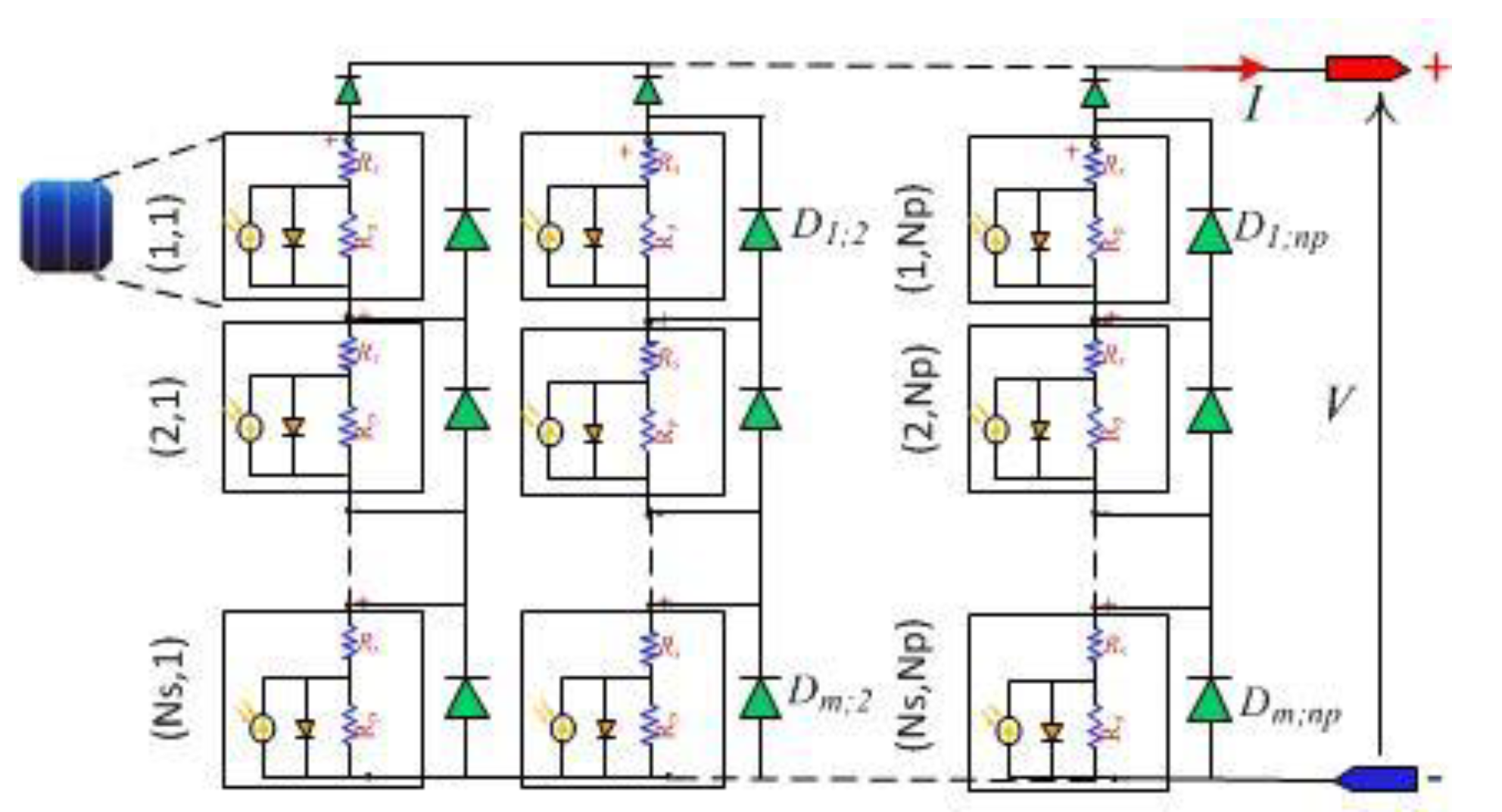
2. Mathematical Models of PV Systems

This section reveals the mathematic model of both the single diode and double diode model (SDM and DDM) topologies that are incorporated in the proposed method.

The SDM is frequently used in the literature because of its simplicity and accuracy in describing the electric cell model. However, the DDM is preferred by some authors owing to its improved accuracy.

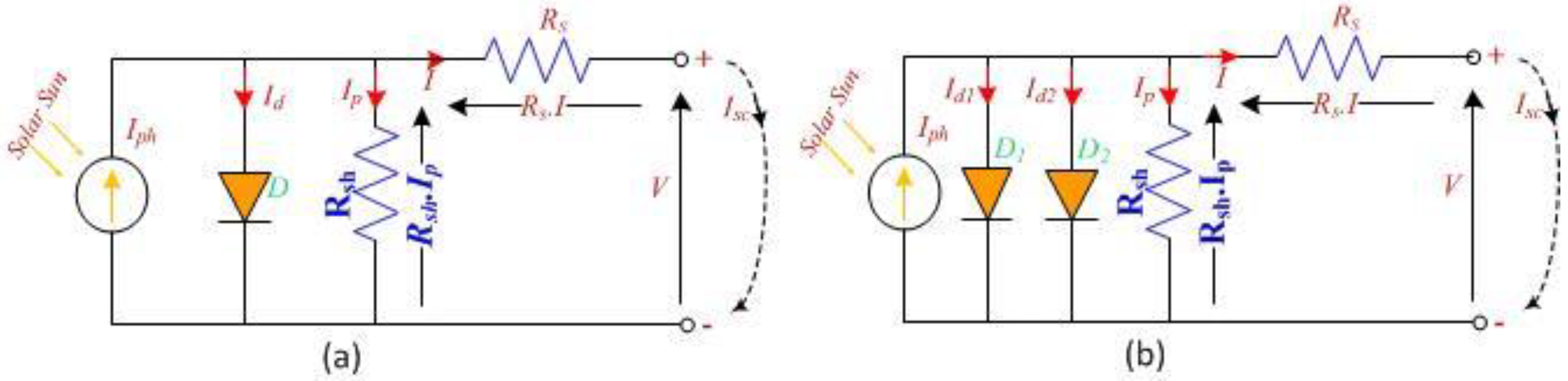
2.1. Single Diode Model Formulation (SDM)

The SDM equivalent circuit utilized in this paper is depicted in Figure 1a.

Its key advantages are its simplicity and accuracy. There were five parameters in this model, and it corresponded to a direct current source connected antiparallel to one diode, including serial R_s and parallel R_sh resistors plugged in at the diode terminal.

For a paired value of illumination and temperature, a conversion of the absorbed light photons to the photocurrent I_ph was conducted. The latter represents the leakage current at the PN junction. Furthermore, the defects presented by the materials at this junction and the losses arising from the different contacts and connections were modeled by the shunt resistance R_sh and series resistance R_s, respectively.

The diode used was characterized by two intrinsic parameters, which were the saturation current I₀ and the ideality factor n. The characteristic I = f(V) generated by the solar cell was obtained by placing a variable load at the output of the cell [34]. The implicit mathematical model obtained by applying Kirchhoff’s laws to the equivalent circuits, with consideration for the electrical parameters of the Shockley’s diode equation, yielded the following Equation (1) as in Reference [23], for the current generated at a specific condition defined by the temperature and irradiance in the PV cell. The equation can be expressed as:

$$I=I_{ph}-I_0\left(e^{q\left(\frac{V+I.R_s}{n.k.T}\right)}-1\right)-\frac{V+I.R_s}{R_{sh}}=f\left(I,V,\phi \right)$$

(1)

where ${\phi }_5=\left(I_{ph},I_0, n,R_s,R_{sh}\right)=\left(x\left(1\right),x\left(2\right), x\left(3\right),x\left(4\right),x(5\right))$, the vector of five unknown parameters. I₀ is the saturation current of the diode, I_ph is the light-generated current, and n is the diode ideality factor. R_s and R_sh are useful gauges for the values of the serial and shunt resistance, k: is the Boltzmann’s constant, and q is the electron charge.

For the double diode model (DDM), the vector of the unknown parameters becomes:

$${\phi }_7=\left(I_{ph},I_0,I_1, n_1,n_2,R_s,R_{sh}\right)=\left(x\left(1\right),x\left(2\right), x\left(3\right),x\left(4\right),x(5\right),x\left(6\right),x\left(7\right)).$$

For the three diode model (TDM), the vector of the unknown parameters becomes:

$${\phi }_9=\left(I_{ph},I_0,I_1,I_2, n_1,n_2,n_3,R_s,R_{sh}\right)=\left(x\left(1\right),x\left(2\right), x\left(3\right),x\left(4\right),x(5\right),x\left(6\right),x\left(7\right),x\left(8\right),x\left(9\right)).$$

In the data sheet of any PV panel, the manufacturer does not provide the five parameters (I₀, I_ph, n, R_s, and R_sh) or the seven or nine parameters, respectively; while only limited experimental data under the standard test conditions (STC) (T = 25 °C, G = 1000 W/m²) are provided. The experimental data provided by the manufacturers includes the (V_oc) [46]: the open-circuit voltage, (I_sc): the short-circuit current, (V_mp): the voltage at the maximum power point, (I_mp): the current at the maximum power point, (b): the open-circuit voltage/temperature coefficient, (a): the short circuit current/temperature coefficient, and (P_max-e): the maximum experimental peak output power.

2.2. Extracting the Five Parameters Under the Standard Test Conditionsfor the Single Diode Model

To rxtract the five parameters of the SDM under STC condition we have to express the short circuit current from Equation (1), that leeds to Equation (2):

$$I_{sc}=I_{ph}-I_0\left(e^{q\left(\frac{I_{sc}.R_s}{n.k.T}\right)}-1\right)-\frac{I_{sc}.R_s}{R_{sh}}$$

(2)

$$I_{ph}\gg I_0\left(e^{q\left(\frac{I_{sc}.R_s}{n.k.T}\right)}-1\right)\gg \frac{{\mathrm{I}}_{\mathrm{sc}}.{\mathrm{R}}_{\mathrm{s}}}{{\mathrm{R}}_{\mathrm{sh}}} \mathrm{then} I_{sc}\approx I_{ph}$$

(3)

Point 1: At the open circuit point (V = V_oc), I = 0. Therefore, Equation (1) can be re-written as:

$$0=I_{ph}-I_0\left(e^{q\left(\frac{V_{oc}}{n.k.T}\right)}-1\right)-\frac{V_{OC}}{R_{sh}}$$

(4)

Additionally, I₀ can be expressed as:

$${\mathrm{I}}_0\approx \frac{I_{ph}-\frac{V_{OC}}{R_{sh}}}{e^{q·\frac{V_{OC}}{n.k.T}}-1};$$

(5)

Considering that$R_{sh}\gg V_{oc}$, Equation (5) gives:

$$I_0\approx \frac{I_{ph}}{e^{q·\frac{V_{OC}}{n.k.T}}-1}$$

(6)

2.3. Extracting the Seven Parameters Under the STC Double Diode Model

To rxtract the seven parameters of the DDM under STC condition we use the same methedology we have to express the short circuit current from Equation (1) and we add one term that refers to the second diode in the model , that leeds to Equation (7):

$$I_{sc}=I_{ph}-I_0\left(e^{q\left(\frac{I_{sc}.R_s}{n1.k.T}\right)}-1\right)-I_1\left(e^{q\left(\frac{I_{sc}.R_s}{n2.k.T}\right)}-1\right)-\frac{I_{sc}.R_s}{R_{sh}}$$

(7)

$$I_{ph}\gg I_0\left(e^{q\left(\frac{I_{sc}.R_s}{n1.k.T}\right)}-1\right)+I_1\left(e^{q\left(\frac{I_{sc}.R_s}{n2.k.T}\right)}-1\right)\gg \frac{I_{sc}.R_s}{R_{sh}} \mathrm{then} I_{sc}\approx I_{ph}$$

(8)

Point 2: At the open circuit point (V = V_oc), I_sc = 0. Therefore, Equation (7) can be re-written as:

Considering that the applied voltage across the diode is V_D = V_oc

$$0=I_{ph}-I_0\left(e^{q\left(\frac{V_{oc}}{n1.k.T}\right)}-1\right)-I_1\left(e^{q\left(\frac{V_{oc}}{n2.k.T}\right)}-1\right)-\frac{V_{oc}}{R_{sh}}$$

(9)

In addition, if we consider that n₁ = n₂ = n, then I_o can be expressed as:

$$I_0\approx I_1\approx \frac{I_{ph}-\frac{V_{OC}}{R_{sh}}}{2(e^{q·\frac{V_{OC}}{n.k.T}}-1)}$$

(10)

Considering that $R_{sh}\gg V_{oc}$, Equation (10) gives:

$$I_0\approx I_1\approx \frac{I_{ph}}{2(e^{q·\frac{V_{OC}}{n.k.T}}-1)}$$

(11)

Figure 2 depicted a diagram illustration of a PV module including a combination of Ns cells connected in series and Np strings connected in parallel (Ns*Np), this configuration is well used to describe the mathematic model behaviors of a solar module or a solar system, a set of modules connected in series and in parallels.

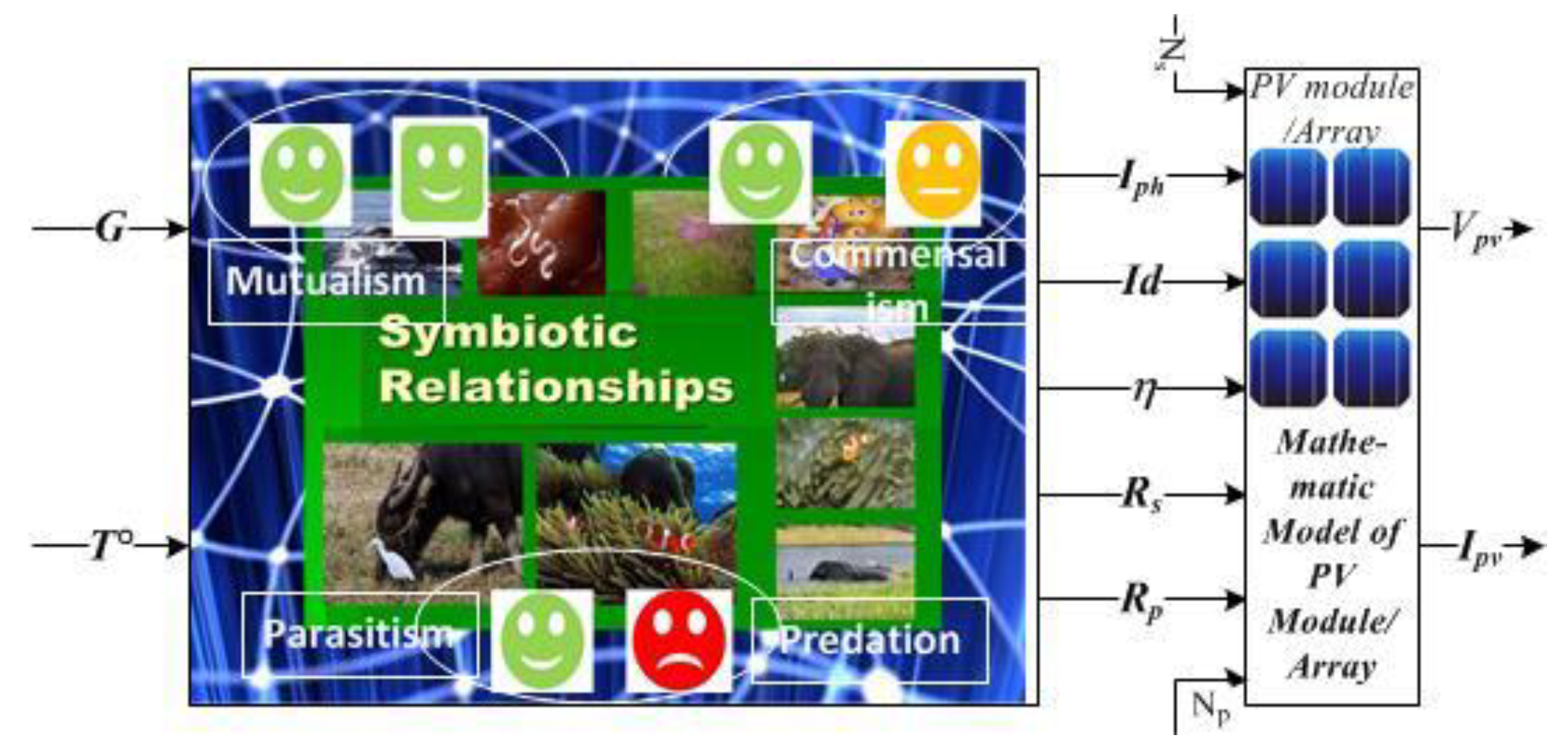
3. Methodology of the Symbiosis Organism Search (DSOS) Algorithm

The current DSOS algorithm mimics the interactive behaviors and the relationships amongst any two distinct organisms in nature or an ecosystem. This relationship is known as symbiosis, and it is characterized by an advantage to the different organisms for the purposes of sustenance and survival. Therefore, symbiosis is the prolonged and mutually beneficial association between organisms.

3.1. Main Idea of the Discrete Symbiotic Organisms Search (DSOS)

In Greek, the word symbiosis means living together. In 1878, De Bary first used the term to explain the cohabitation between two different species.

A symbiotic relationship may be obligatory when a pair of organisms depends on each other for survival or it may be facultative when the two organisms cohabitate in a mutually beneficial manner without a relationship.

Examples of symbiotic relationships found in an ecosystem can be mutualism, commensalism, predation, or parasitism, although in general, predation is considered as a kind of parasitism.

When benefits to both govern the relationship between two distinct species, we talk about mutualism, for example, the pollination with a bee or when a small crab that lives in a mussel receives protection and food, while the inside of the mold is cleaned by the crab. However, both can also live separated.

Commensalism is a relationship in an ecosystem between two different organisms where one benefits and the other is neutral or unaffected, for example, the jackal feeds on the remains of prey left by the lions.

Finally, parasitism defines a relationship of paired distinct species on which one benefits at the expense of the second, which is harmed. For example, end parasites in humans and the disease they cause, that is, Malaria.

Figure 3 depicts a set of the symbiotic organisms in the same ecosystem, where the relationship in an ecosystem is dynamic and the organism develops many tools to adapt to a change in their environment. Therefore, from the time that it is built, the symbiotic relationship continues to shape and sustain all changes in the ecosystem.

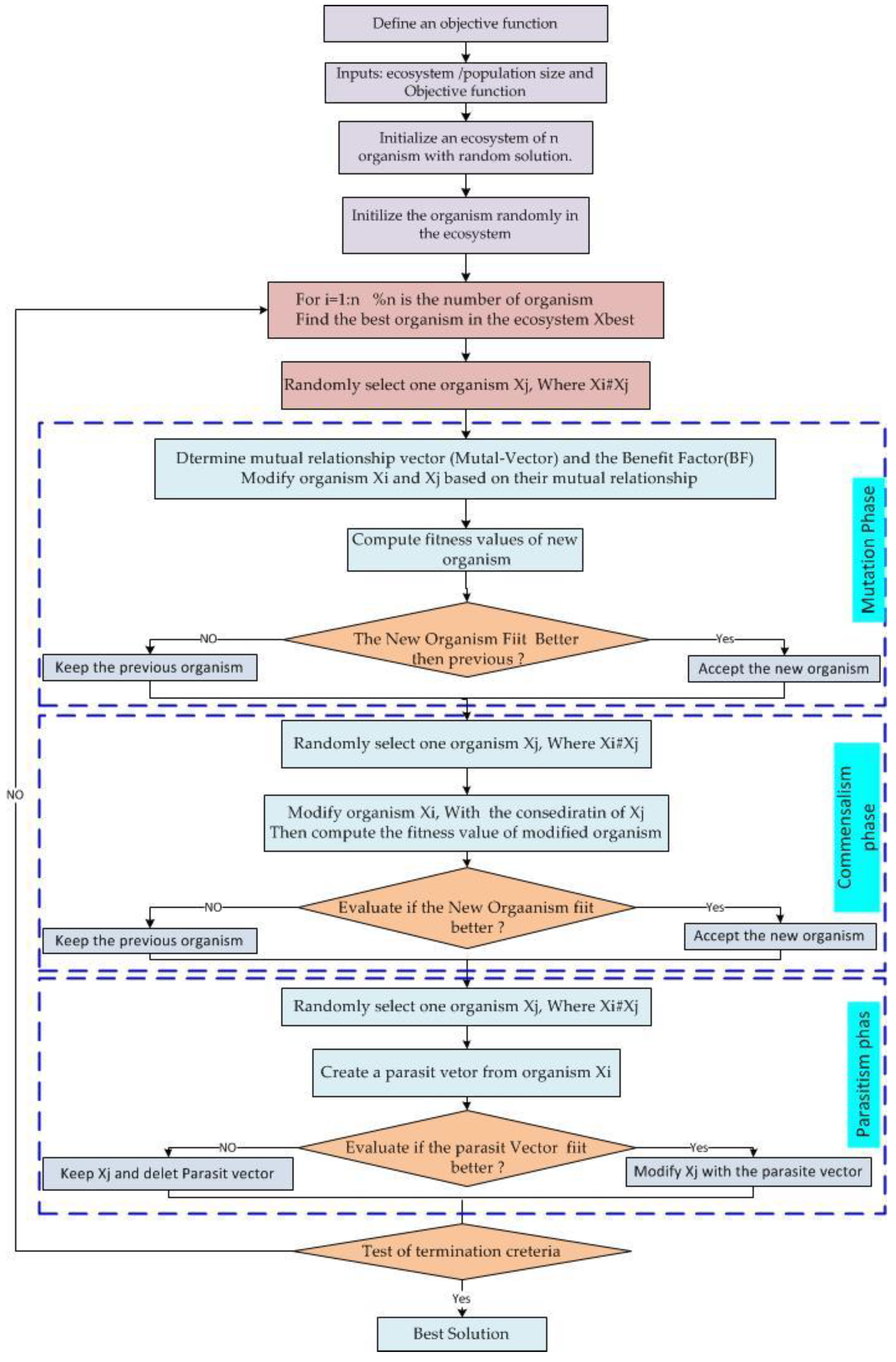
3.2. Flowchart of the DSOS

The working principle of the DSOS is presented in the flow chart Figure 4, the algorithm starts with an objective function to be defined by the user several inputs describing the ecosystem, as well as an initialization of a set of n random solutions.

The description of the principal of this flow chart is presented in Section 3.3. and the computational procedure in Section 3.4.

3.3. The Discrete Symbiotic Organisms Search Algorithm (DSOS)

DSOS-based algorithms imitate symbiotic interactions between a couple of organisms in the same ecosystem. In the optimization problem, each organism denotes a potential solution, and it is totally defined by its position in the solution space.

Like all population-based algorithms, the DSOS iteratively uses a population of candidate solutions in the search space to search for a global solution.

In each iteration, all the organisms adjust their position according to the mutualism, commensalism, and parasitism biological interaction models of the ecosystem.

The first set of organisms or population is called an ecosystem, and it is randomly generated. Every candidate in this ecosystem represents a solution for the given optimization problem, and each candidate in the ecosystem has a fitness value which reflects the degree of appurtenance to the aimed objective.

This algorithm is different from other heuristic algorithms in that the GA needs two tuning parameters, that is, the cross over and mutation rate, while the harmony search needs three rules to adjust and improvise new harmony, being memory consideration, pitch adjustment, and random choosing. Meanwhile, in the ABC algorithm, three phases are introduced to find the best food source, that is, the employed bee, the onlooker bee, and the scout bee phases.

In the current algorithm (DSOS), three phases need to be considered, that is, the mutualism phase, commensalism phase, and the parasitism phase.

Therefore, the process of the basic code of the DSOS algorithm is as follows:

Initialization (eco-size, initial population, stopping criteria);

REPEAT (for all organisms in the ecosystem)

• Determine the best organism,
• Mutualism phase: % interaction benefit for both sides,
• Commensalism phase: % benefit to one side and the other side is neutral.
• Parasitism phase: % benefit to one side and the other is well harmed.

UNTIL the stopping criteria is met.

For a further theoretical approach, the next section describes how these three phases are described mathematically.

3.3.1. Mutualism

Given a set of bees and flowers in an ecosystem, both organisms have a mutual benefit.

X_i denotes an organism matched to the ith member of the ecosystem (for example, the ith bee). Another organism is X_j, which denotes a flower selected randomly. The pair (X_i, X_j) engages in a mutualistic relationship, where both organisms engage with a goal of the increased chance of survival in the ecosystem.

A new candidate solution X_new for the paired X_i and X_j, is calculated based on the mutualistic symbiosis for both X_i and X_j as follows: Equations (12) and (13).

$$X_{i-new}=X_i+rand(0,1)\times \left(X_{best}-Mutual\_Vector\times B{F}_1\right).$$

(12)

$$X_{j-new}=X_j+rand(0,1)\times \left(X_{best}-Mutual\_Vector\times B{F}_2\right).$$

(13)

$$Mutual\_Vector=(0.5)\times (X_i+X_j).$$

(14)

where rand (0, 1) is a vector of a random number.

In nature, some mutualistic relationships grant a greater beneficial advantage to one organism than to another. Therefore, to emulate this inequality of benefits, the benefit factors BF₁ and BF₂ have been introduced in Equations (1) and (2), so that these factors represent the level of benefit to each organism in the adverse situation.

Equation (3) represents the relationship characteristics between organisms X_i and X_j, such that the part of the equation:

(X_best − Mutual_Vector*BF₁),

reflects the mutualistic effort to increase their survival advantages. X_best represents the highest degree of adaptation, and each organism is updated only if their new fitness is better than pre-interaction fitness, in other words, every organism is forced to increase their degree of adaptation to their ecosystem as described in Reference [36].

3.3.2. Commensalism

Similar to the mutualism phase, an organism X_j is randomly selected from the ecosystem to interact with X_i.

X_i attempts to benefit from this relationship; however, organism X_j is neither benefiting nor being harmed. The Xnew is calculated according to this commensalism symbiosis relation and can be modeled using Equation (15).

The part of the equation (X_best−X_j) reflects the beneficial advantage provided by X_j to help X_i increase its survival advantages, to a higher degree if the organism is to fit X_best.

The organism X_i-new is replaced by X_i only if the latter is better.

3.3.3. Parasitism

In the parasitism phase, for each organism i denoted as X_i, another different organism j denoted as X_j is randomly selected. An artificial parasite X_i-new is produced by first duplicating organism X_i, and then modifying the randomly selected dimension d by replacing the current value with a randomly generated value between the minimum and the maximum of the corresponding dimensions. In other words:

$$X_{i\_new}=\{\begin{array}{ll}{X}_{i,k}& if\hspace{1em}k\ne d\\ X_{\min ,k}+rand(0,1)\times \left(X_{\max ,k}-X_{\min ,k}\right)& if\hspace{1em}k=d \end{array}.$$

(15)

The randomly selected X_j serves as a host to the artificial parasite X_i. If the artificial parasite is better than the host X_j, then X_j is killed and the artificial parasite takes place of the killed organism.

In other words, both organisms have to evaluate their fitness value, and if the parasite-vector has a better fitness value, it will kill organism X_j and take its place in the ecosystem. However, if the fitness value of the organism X_j is better, then X_j has immunity from the parasite (for example, immunity from Malaria) and the parasite-vector will no longer be able to live in that ecosystem.

3.4. Computation Procedure of the DSOS Algorithm

To implement the DSOS method and evaluate the effectiveness, below we depict the code of the DSOS algorithm (Algorithm 1).

Algorithm 1 Code of the DSOS algorithm

Define an objective function f(X); X = (x1, x2, x3,…,xd) %d is the dimension  % of the problem  Inputs: ecosystem/population size and the objective function  Initialize an ecosystem of n organisms with a random solution.  % Initialize the organism randomly in the ecosystem  % Evaluate the fitness of the new solution  % Increase the number of function evaluation count.  While (t < Ecosystem)  For i = 1:n % n is the number of organisms  Find the best organism in the ecosystem Xbest    % Mutation phase  Randomly select one organism Xj, where Xi # Xj Determine the mutual relationship vector (Mutual-Vector) and the benefit factor (BF). Modify organism Xi and Xj using Equations (12)–(14).  If the modified organism gives a better fitness evaluation than the previous one, then update them in the ecosystem.    % Commensalism phase  Randomly select one organism Xj, where Xi # Xj  Modify organism Xi and Xj using Equation (15)  If the modified organism gives a better fitness evaluation than the previous: then update them in the ecosystem.    % Parasitism phase  Randomly select one organism Xj, where Xi # Xj  Generate a parasite vector from organism Xi (Equation (15))  If the parasite-vector gives a better fitness evaluation than Xj, then replace it with the parasite-vector in the ecosystem.  End for  Then the Global Best solution is saved as an optimal solution; End while

3.5. Formulation of the SDM Solar Cell Parameter Estimation Problem

Many electric models for the solar cell have been proposed to describe the I-V characteristics. The main circuit models are the single diode and double diode models.

3.5.1. Single Diode Model Formulation SDM

At the maximum point, V = V_mp and I = I_mp. At the maximum power point, Equation (1) can be re-written as:

$$I_{mp}=I_{ph}-I_0\left(e^{q\left(\frac{V_{mp}+I_{mp}.R_s}{n.k.T}\right)}-1\right)-\frac{V_{mp}+I_{mp}.R_s}{R_{sh}},$$

(16)

Differentiation gives:

$$\frac{dI}{dV}=-I_0\times \left[\frac{q}{n·k·T}·\left(1+\frac{dI}{dV}·R_s\right)e^{q·\left(\frac{V+I.R_s}{n.k.T}\right)}\right]-\frac{1}{R_{sh}}\times \left(1+\frac{dI}{dV}·R_s\right),$$

(17)

We have to calculate this amount at different points on the characteristic:

At the short circuit point (V = 0; I = I_sc). Applying the short circuit condition to Equation (17), we obtain:

$${\frac{dI}{dV}|}_{V=0}=-I_0\times \left[\frac{q}{n·k·T}·\left(1+{\frac{dI}{dV}|}_{V=0}·R_s\right)e^{q·\left(\frac{I_{sc}.R_s}{n.k.T}\right)}\right]-\frac{1}{R_{sh}}·\left(1+{\frac{dI}{dV}|}_{V=0}·R_s\right),$$

(18)

At the open circuit point (V = V_oc); I = 0. Equation (17) can also be written as:

$$\begin{gathered} {\frac{dI}{dV}|}_{I=0}=-I_0\times \left[\frac{q}{n·k·T}·\left(1+{\frac{dI}{dV}|}_{I=0}·R_s\right)e^{q·\left(\frac{V_{oc}}{n.k.T}\right)}\right]-\frac{1}{R_{sh}} \\ ·\left(1+{\frac{dI}{dV}|}_{I=0}·R_s\right) \end{gathered}$$

(19)

The derivative of the solar PV power with respect to the voltage gives the last independent equation. This derivative is equal to zero at the maximum power point, and it is obtained as:

$$\frac{dP}{dV}=\frac{d\left(I·V\right)}{dV}=I+\frac{dI}{dV}·V=0 \leftrightarrow \frac{I}{V}=-\frac{dI}{dV}$$

(20)

So at the MPP (V = V_mp and I = I_mp), Equation (17) becomes:

$${\frac{\mathrm{dI}}{\mathrm{dV}}|}_{\left({\mathrm{V}}_{\mathrm{mp}},{\mathrm{I}}_{\mathrm{mp}}\right)}=-\frac{{\mathrm{I}}_{\mathrm{mp}}}{{\mathrm{V}}_{\mathrm{mp}}},$$

(21)

The substitution of Equation (21) in to Equation (17) gives:

$$-\frac{I_{mp}}{V_{mp}}=-I_0\times \left[\frac{q}{n·k·T}·\left(1-\frac{I_{mp}}{V_{mp}}·R_s\right)\right]-\frac{1}{R_{sh}}\times \left(1-\frac{I_{mp}}{V_{mp}}·R_s\right),$$

(22)

We note $R_{s0}$ and $R_{sh0}$ as:

$${\frac{\mathrm{dI}}{\mathrm{dV}}|}_{\mathrm{V}={\mathrm{V}}_{\mathrm{oc}}}={\mathrm{R}}_{\mathrm{s}0},$$

(23)

$$\mathrm{And} {\frac{dI}{dV}|}_{I=I_{sc}}=R_{sh0} ,$$

(24)

To get the vector of the five parameters we have to solve Equations (2), (4), (7), (8), and (13).

3.5.2. Double Diode Model Formulation (DDM)

The implicit mathematical model obtained by applying Kirchhoff’s laws to the equivalent circuits, with consideration for the electrical parameters of the two Shockley’s diode equations, gives the following equation for the current generated in the PV cell at a particular operating point.

The equation can be expressed as:

$$I=I_{ph}-I_{01}\left(e^{q\left(\frac{V+I.R_s}{n_1.k.T}\right)}-1\right)-I_{02}\left(e^{q\left(\frac{V+I.R_s}{n_2.k.T}\right)}-1\right)-\frac{V+I.R_s}{R_{sh}}=f\left(I,V,\phi \right),$$

(25)

where$\phi =\left(I_{01},I_{02},I_{ph}, n_1,n_2,R_s,R_{sh}\right)$, represents the vector of seven unknown parameters.

3.6. Parameter Optimization Problem for SDM and DDM

To identify the intrinsic parameter of the vectors $\phi =\left(I_0, I_{ph}, n, R_s, R_{sh}\right)$ for the SDM, it is described using Equation (1) or $\phi =\left(I_{01}, I_{02}, I_{ph}, n_1,n_2, R_s,R_{sh}\right)$ For the DDM, it was described using Equation (13), and we fitted the best model described by either Equation (1) or Equation (13) to the experimental data V = g(I). Through minimization of the squared error of the theoretical and experimental curves, we defined an objective function (OF) that evaluated the degree of correspondence between the estimated and calculated parameters as a sum of the squared errors (SSE), which is given by:

$$g\left(I,V,\phi \right)={\displaystyle \sum }_{k=1}^N{\left[I_{mes,k}-f_k\left(I,V,\phi \right)\right]}^2={\displaystyle \sum }_{k=1}^N{\left(\Delta E_k\right)}^2$$

(26)

$$\Delta E_k=\left|I_{measured,k}-I_{ calculated,k}\right|$$

(27)

Theoretically, the (OF) value should be zero when the best values of the parameters are obtained, and estimated to fit the experimental results.

$I_{mes,k}$is the k_th measurement data of I_pv.

$\Delta E_k$ is the absolute error between $I_{mes,k}$ and $I$ _calculated $=f\left(I,V,\phi \right)$from Equation (1).

$\phi =\left(I_{ph,}{I}_0, n,R_s,R_{sh}\right)$: Vector of the five unknown intrinsic parameters for the SDM.

$\phi =\left(I_{ph,}{I}_{01},I_{02}, n_1,n_2,R_s,R_{sh}\right)$: Vector of the seven unknown intrinsic parameters for the DDM.

N is the number of measurement points.

Objective: The minimum of the SSE leads to optimal values of the parameters: $\phi ={\phi }_{opt}$.

The optimization of the objective function cannot be done analytically due to the non-linearity of the characteristic I = g(V), and due to the difficulty for the structural parameters R_s and n to be expressed in the exponential term. As a consequence, the numerical method based on the last square principal was more appropriate to minimize such a function.

Various evaluation criteria have been used in the literature to qualify the accuracy and effectiveness of the proposed optimization algorithm based on a statistical approach.

The relative error (RE): this factor is based on the error between the extracted and the measured parameter set. It has been used in previous research to calculate and compare the accuracy of the optimization method.

$$RE=\left|\frac{I_{measured,k}-I_{ calculated,}}{I_{ measured,k}}\right|$$

(28)

The root mean square error (RMSE): This criterion compares the experimental and the calculated or fitted data, and it gives an error as the output.

$$RMSE=\sqrt{\frac{1}{N}{\displaystyle \sum }_{\mathrm{k}=1}^{k=N}{\left|I_{measured,k}-I_{calculated,k}\right|}^2 }=\sqrt{\frac{1}{N}{\displaystyle \sum }_{k=1}^{k=N}{\left[g_k\left(I_k,V_k,\phi \right)\right]}^2}$$

(29)

The normalized deviation as described in Reference [47].

$$D(\%)=\frac{1}{100}*\left(\frac{I_{measured,k}-I_{calculated,k}}{I_{measured,k}}\right)$$

(30)

Several other statistical parameters have been used in the literature to demonstrate the effectiveness and the competitiveness of the optimization method.

Examples of statistic variables that have been used include the normalized mean square error (NMSE), root mean square deviation (RMSD), normalized root mean square deviation (NRMSD), mean absolute error (MAE), mean absolute error in power (MAEP), mean bias error (MBE), mean square error (MSE), sum square error (SSE), residual error of the fitness function (REFF), absolute error (AE), mean relative error (MRE), coefficient of determination (R²), mean absolute bias error (MABE), mean absolute percentage error (MAPE), individual absolute error (IAE), error between simplified parameters (ESP), and the absolute current error (ACE).

3.7. Symbiosis Organism Search Implementation

Statistical errors were evaluated to check the accuracy of the proposed method. The statistic variables used include the: absolute error (AE), mean absolute error (MAE), root mean squared error (RMSE), and the weighted RSME proposed in Reference [48]. One or more of these parameters were calculated and compared for the different methods.

$$AE={\displaystyle \sum }_{k=1}^{k=N}\left|I_{measured,k}-I_{calculated,k}\right|$$

(31)

$$MAE=\frac{1}{N}{\displaystyle \sum }_{k=1}^{k=N}\left|I_{measured,k}-I_{calculated,k}\right|$$

(32)

$$SSE={\displaystyle \sum }_{k=1}^{k=N}{\left|I_{measured,k}-I_{calculated,k}\right|}^2$$

(33)

$$RMSE=\sqrt{\frac{1}{N}{\displaystyle \sum }_{k=1}^{k=N}{\left|I_{measured,k}-I_{calculated,k}\right|}^2 }=\sqrt{\frac{1}{N}{\displaystyle \sum }_{k=1}^{k=N}{\left(\Delta E_k\right)}^2}$$

(34)

$$NRMSD=\frac{RMSD}{I_{sc}}\times 100\%$$

(35)

$$\xi =\frac{RMSE}{I_{sc}}=\frac{1}{I_{sc}}\sqrt{\frac{1}{N}{\displaystyle \sum }_{k=1}^{k=N}{\left|I_{measured,k}-I_{calculated,k}\right|}^2 }=\frac{1}{I_{sc}}\sqrt{\frac{1}{N}{\displaystyle \sum }_{k=1}^{k=N}{\left(\Delta E_k\right)}^2}$$

(36)

3.8. Measurement and Experiment Results

To illustrate the effectiveness of the symbiosis organism search method in determining the five electrical parameters of the solar cell data, it was necessary to establish and situate the current study versus relevant previous works, and to highlight the effectiveness of the SOS method.

The data cited in Reference [47] by (T. EASWARAKHANTHAN and all (1986)) was measured from a PWP-201 type Photowatt panel, including 36 polycrystalline Silicon cells connected in series, operating under a 1000 w/m² solar irradiance and at 45 °C.

A second case was studied and it referred to a 57 diameter commercial (R, T, C France) Silicon solar panel, under 1000 w/m² and at 33 °C temperature.

The third case concerned the Sharp ND-R250A5 PV module, where the electrical characteristics of this module were I_sc = 8.68 A, V_oc = 37.6 V, I_mpp = 8.10 A, and V_mpp = 30.9 V. This panel contained 60 polycrystalline silicon cells connected in series under 1040 w/m² and at 59 °C. The 36 measurements were cited in Reference [3].

The data were obtained through measurements performed on one cell at 33°C and one module at 45°C using a single diode model of a photovoltaic module. The technical characteristics of the cell and the module used are shown in

Table 1. Cell and module parameters of the single diode model.

	Cell (33 °C)	Module (45 °C)
Iph (A)	0.7608	1.0318
Is ($\mathsf{\mu }$A)	0.3223	3.2876
Gsh (£−1)	0.0186	0.0018
Rs (£−)	0.0364	1.2057
n	1.4837	48.4500
$\sigma (\%)$	0.6251	0.7805
Isc (A)	0.7603	1.0300
Voc (V)	0.5728	16.7780
Vm (V)	0.4507	12.6790
Im (A)	0.6894	0.9120
FF	0.7135	0.6680

.

3.8.1. Simulation and experimental results of the Single Diode Model

Table 2. Comparison of the experimental measurement and computed data from the solar cell (Photowatt-PWP201 PV Cell) at 33 °C.

N°	Vimes (V)	Iimes (A)	${\widehat{\mathit{I}}}_{\mathrm{cal}}$ (DOSE)	IAE ‘DSOS’	D (%)	IAE LMSA	IAE GGHS	IAE ABSO	IAE CPSO
1	−0.2057	0.7640	0.7661000	0.002100	−0.013	11.5761 × 10−5	25.4092 × 10−5	19.9357 × 10−5	27.2179 × 10−5
2	−0.1291	0.7620	0.7631000	0.001100	−0.091	68.0671 × 10−5	81.1919 × 10−5	73.5839 × 10−5	43.0953 × 10−5
3	−0.0588	0.7605	0.7611000	0.000600	−0.118	86.3281 × 10−5	98.8025 × 10−5	89.2356 × 10−5	74.0421 × 10−5
4	0.0057	0.7605	0.7602720	0.000228	0.039	34.6856 × 10−5	22.8090 × 10−5	34.1728 × 10−5	35.3308 × 10−5
5	0.0646	0.7600	0.7591460	0.000854	0.118	95.3669 × 10−5	84.0396 × 10−5	97.0345× 10−5	85.4218 × 10−5
6	0.1185	0.7590	0.7585000	0.000500	0.132	97.3813 × 10−5	86.5670 × 10−5	101.025 × 10−5	77.8602 × 10−5
7	0.1678	0.7570	0.7575000	0.000500	−0.013	69.0271 × 10−5	17.2188× 10−5	1.50171 × 10−5	34.8729 × 10−5
8	0.2132	0.7570	0.7562120	0.000788	0.119	88.6778 × 10−5	78.8905 × 10−5	95.5786 × 10−5	53.6411 × 10−5
9	0.2545	0.7555	0.7560000	0.000500	0.051	44.53071× 10−5	35.3713× 10−5	52.5346× 10−5	4.61184× 10−5
10	0.2924	0.7540	0.7541000	0.000100	0.040	37.01388× 10−5	28.7037× 10−5	45.5357 × 10−5	45.0681 × 10−5
11	0.3269	0.7505	0.7516000	0.001100	−0.120	85.8429 × 10−5	92.9424 × 10−5	77.6748 × 10−5	124.115 × 10−5
12	0.3585	0.7465	0.7472610	0.000761	−0.107	82.7345 × 10−5	88.1240 × 10−5	76.0912 × 10−5	111.361 × 10−5
13	0.3873	0.7385	0.7392600	0.000760	−0.217	160.213 × 10−5	163.391 × 10−5	156.431 × 10−5	172.219 × 10−5
14	0.4137	0.7280	0.7285100	0.000510	0.082	61.6337 × 10−5	60.9190 × 10−5	61.3997 × 10−5	71.5867 × 10−5
15	0.4373	0.7065	0.7073010	0.000801	−0.071	49.2923 × 10−5	47.9481 × 10−5	53.8447 × 10−5	17.5705 × 10−5
16	0.4590	0.6755	0.6753990	0.000101	0.015	18.2486 × 10−5	20.3482 × 10−5	10.3140 × 10−5	63.6238 × 10−5
17	0.4784	0.6320	0.6312000	0.000800	0.190	119.491 × 10−5	120.108 × 10−5	110.694 × 10−5	161.040 × 10−5
18	0.4960	0.5730	0.5730000	0.000000	0.140	102.652 × 10−5	99.2188 × 10−5	96.3482 × 10−5	118.099 × 10−5
19	0.5119	0.4990	0.4992000	0.000200	−0.080	63.89021 × 10−5	73.4145 × 10−5	16.4603 × 10−5	94.8217 × 10−5
20	0.5265	0.4130	0.4141000	0.001100	−0.097	65.7580 × 10−5	82.6002 × 10−5	243.286 × 10−5	158.721 × 10−5
21	0.5398	03165	0.3170100	0.000510	−0.221	99.2379 × 10−5	122.715 × 10−5	18.4533 × 10−5	255.847 × 10−5
22	0.5521	0.2120	0.2121610	0.000161	−0.236	11.2783 × 10−5	39.2380 × 10−5	15.6971 × 10−5	222.111 × 10−5
23	0.5633	0.1035	0.1022000	0.001300	0.870	130.599 × 10−5	102.001 × 10−5	154.636 × 10−5	111.047 × 10−5
24	0.5736	−0.010	−0.009230	0.000770	3.000	122.858 × 10−5	146.201 × 10−5	103.23 × 10−5	354.617 × 10−5
25	0.5833	−0.123	−0.124300	0.001300	−0.894	254.525 × 10−5	240.977 × 10−5	272.460 × 10−5	61.7820 × 10−5
26	0.590	−0.21	−0.20750	0.00250	0.334	152.25 × 10−5	152.95 × 10−5	155.92 × 10−5	273.84 × 10−5

depict a comparison between the individual absolute error (IAE) of experiment measurement and computed data using DSOS, LMSA, GGHS, ABSO and CPSO, however

Table 3. Results obtained from different optimization methods using the SDM for the commercial solar cell. (Photowatt-PWP201 PV Cell) at 33 °C.

	Iph (A)	I0 ($\mu A$)	n	Rs (£)	Rsh (£)	SSE	RMSE	$\xi$
GA [49]	0.76190	0.80870	1.57510	0.02990	42.3729	9.4632 × 10−3	1.9078 × 10−2	2.51 × 10−2
SA [50]	0.76200	0.47980	1.51720	0.03450	43.1034	9.3839 × 10−3	1.8998 × 10−2	2.50 × 10−2
PS [51]	0.76170	0.99800	1.60000	0.03130	64.1026	5.8005 × 10−3	1.4936 × 10−2	1.96 × 10−2
NR [47]	0.76080	0.32230	1.48370	0.03640	53.7634	2.4445 × 10−3	9.6964 × 10−3	1.28 × 10−2
DE [52]	0.76080	0.32300	1.48060	0.03640	53.7185	1.4265 × 10−4	2.3423 × 10−3	3.08 × 10−3
CPSO [53]	0.76070	0.40000	1.50330	0.03540	59.0120	4.9952 × 10−5	1.3861 × 10−3	1.82 × 10−3
ABSO [38]	0.76080	0.30620	1.47580	0.03660	52.2903	2.5547 × 10−5	9.9124 × 10−4	1.30 × 10−3
GGHS [54]	0.76090	0.32620	1.48220	0.03630	53.0647	2.5528 × 10−5	9.9097 × 10−4	1.30 × 10−3
LMSA [34]	0.76078	0.31849	1.47976	0.03643	53.3264	2.5297 × 10−5	9.8640 × 10−4	1.30 × 10−3
IADE [55]	0.76070	0.33613	1.48520	0.03621	54.7643	9.8900 × 10−4	6.1706 × 10−3	8.12 × 10−3
TLBO [42]	0.76074	0.32378	1.48136	0.03641	54.4029	9.8845 × 10−4	6.1689 × 10−3	8.11 × 10−3
STLBO [42]	0.76078	0.32302	1.48114	0.03638	53.7187	9.8602 × 10−4	6.1613 × 10−3	8.10 × 10−3
DSOS (current Method)	0.759533	0.195478	1.4526	0.0392996	72.7785	1.20836 × 10−5	4.5918 × 10−4	3.48943 × 10−3

The bold values in the last line are the calculated values of the five parameters obtained from the symbiotic organism search (SOS). The best fitness value of the objective function is 4.5918 × 10⁻⁴. The bold value in the RMSE colon is the best result obtained with the correspondent algorithm.

presents a comparaison between SSE and RMSE of DSOS versus 12 different stockastique methods from previous research.

The Figure 5 depict the value of the objective function minimized for each parameters of the Photowatt solar cell and Figure 6 presents the individual absolute error (IAE) a comparison between different methods.

The objective function OF needs to be minimized to find the optimal set of parameters that describe the electrical characteristics of the solar cell.

Table 4. Lower and upper bounds of the five parameters for the solar cell.

Parameters	Iph (A)	${\mathit{I}}_0 \left(\mathit{\mu }\mathit{A}\right)$	n	Rs (£)	Rsh (£)
Lower	0.5	0	1	0	50
Upper	1	0.5	1.5	0.5	100

present Lower and upper bounds of the five parameters for the solar cell and

Table 5. Comparison of the experimental measurements and the computed data from the module array: (Photowatt-PWP201 PV Module) at 45 °C.

N°	Vi (V)	Ii (A)	Îcal ‘DSOS’	IAE ‘DSOS’	D (%)	IAE “PS”	IAE “GA”	IAE “Bouzidi”
1	−1.9426	1.0345	1.033	0.00150	0.184	---	---	---
2	0.1248	1.0315	1.031	0.00050	0.126	0.002135	0.010190	7.7476 × 10−5
3	1.8093	1.0300	1.028	0.002000	0.175	0.003030	0.00869848	0.00164534
4	3.3511	1.0260	1.0262	0.000200	−0.029	0.001267	0.00991153	0.00049525
5	4.7622	1.0220	1.024	0.002000	−0.235	0.000558	0.01122849	0.00077184
6	6.0538	1.0180	1.022	0.004000	−0.432	0.002262	0.01245763	0.00197105
7	7.2364	1.0155	1.02	0.004500	−0.433	0.001986	0.01172839	0.00124347
8	8.3189	1.0140	1.016	0.002000	−0.217	0.000419	0.008880327	0.00155399
9	9.3097	1.0100	1.0123	0.002300	−0.020	0.002528	0.00632724	0.00398586
10	10.2163	1.0035	1.001	0.002500	0.309	0.006023	0.00237690	0.00772169
11	11.0449	0.9880	0.9852	0.002800	0.364	0.006603	0.00133367	0.00844289
12	11.8018	0.9630	0.9608	0.002200	0.363	0.006499	0.00097747	0.00836817
13	12.4929	0.9255	0.9245	0.001000	0.270	0.005437	0.00160795	0.00721723
14	13.1231	0.8725	0.8742	0.001700	−0.012	0.002350	0.00432213	0.00393147
15	13.6983	0.8075	0.8086	0.00110	0.012	0.002308	0.00407491	0.00359833
16	14.2221	0.7265	0.7286	0.00210	−0.220	0.000119	0.00630370	0.00082416
17	14.6995	0.6345	0.6363	0.00175	−0.331	0.001255	0.00732234	0.00068144
18	15.1346	0.5345	0.5347	0.00020	−0.243	0.000617	0.00662565	0.00040412
19	15.5311	0.4275	0.4272	0.00030	−0.327	0.001154	0.00712186	0.00126106
20	15.8929	0.3185	0.3167	0.00180	−0.063	0.000390	0.00553537	1.3616 × 10−5
21	16.2229	0.2085	0.2059	0.00260	0.336	0.001615	0.00423231	0.00103447
22	16.5241	0.1010	0.0966	0.000444	2.673	0.005205	0.00052532	0.0044828
23	16.7987	−0.008	−0.0095	0.00148	−2.500	0.000561	0.00495155	0.00022555
24	17.0499	−0.111	−0.1116	0.00060	0	0.000051	0.00524400	0.00075112
25	17.2793	−0.209	−0.2089	0.00010	−0.048	0.000244	0.00470115	0.00052498
26	17.4885	−0.303	−0.3009	0.00210	0.330	0.002267	0.00683625	0.00295655

show a Comparison of the experimental measurements and the computed data from the module array: (Photowatt-PWP201 PV Module) at 45 °C. however

Table 6. Results obtained from the different optimization methods using the SDM for the module array: (Photowatt-PWP201 PV module) at 45 °C.

	Iph(A)	${\mathit{I}}_0 \left(\mathit{\mu }\mathit{A}\right)$	n	Rs (£)	Rsh (£)	RMSE	$\mathit{\xi }$
GA [56]	1.0441	3.4360	1.34962	1.1968	555.556	Nc	Nc
PS [56]	1.0313	3.1756	1.34136	1.2053	714.286	0.0118	1.96 × 10−2
El Nagaar [51]	1.0331	3.6642	1.35614	1.1989	833.333	2.9251 × 10−3	2.48 × 10−3
Peng [57]	1.0313	3.2212	1.34228	1.2132	625.000	6.3448 × 10−0.3	7.49 × 10−3
Cong [58]	1.0305	3.4823	1.35118	1.2013	981.982	2.266 × 10−3	2.20 × 10−3
Bouzidi [59]	1.0339	3.0760	1.33850	1.2030	555.556	4.0067 × 10−3	3.89 × 10−3
Al Hajri [51]	1.0313	3.1756	1.34135	1.2053	714.286	3.3269 × 10−3	3.23 × 10−3
Phang [8]	1.0319	64.0490	1.76024	0.0832	561.034	3.5432 × 10−3	3.44 × 10−2
Cubas [48]	1.0342	1.3214	1.25543	1.3535	559.680	2.9355 × 10−3	2..85 × 10−3
(DSOS)	1.0338	3.1488	1.4139	1.2135	773.380	5.752 × 10−4	T = 259 ms

deoict a comparaison of the numerical results obtained from 9 various optimization methods published earlier using the SDM for the module array: (Photowatt-PWP201 PV module) at 45 °C.

Table 7. Lower and upper bounds of the five parameters for the solar module array: (Photowatt-PWP201 PV Module) at 45 °C.

Parameters	Iph (A)	${\mathit{I}}_0 \left(\mathit{\mu }\mathit{A}\right)$	n	Rs (£)	Rsh (£)
Lower	0.01	0.01	0.01	0.001	0.001
Upper	1.2	5	2	2	5000

depict Lower and upper bounds of the five parameters for the solar module array: (Photowatt-PWP201 PV Module) at 45 °C. this interval is mandatory to have a good convergence in a few iteration .

Table 8. Comparison of the experimental measurements and the computed data from the module array: (Sharp ND R250 A5 PV Module), at 1040 w/m² and 59 °C.

N°	Vi(V)	Ii(A)	Ical (DSOS)	IAE (DSOS)	Ical (GCPSO)	IAE (GCPSO)
1	0.000	9.1500	9.1458000	0.00422953	9.14377047	0.00622953
2	7.7100	9.1400	9.1399000	0.00013317	9.14168233	0.00168233
3	10.9800	9.1200	9.12596243	0.00596243	9.13887739	0.01887739
4	14.5500	9.1100	9.1134749	0.0034749	9.12574851	0.01574851
5	16.3600	9.1000	9.10148715	0.00148715	9.10450087	0.00450087
6	18.0000	9.0700	9.06698347	0.00301653	9.06239347	0.00831337
7	19.1500	9.0200	9.01188479	0.00811521	9.00539847	0.01460153
8	20.0400	8.9500	8.94512790	0.00487210	8.93702852	0.01297148
9	20.8700	8.8600	8.85488479	0.00511521	8.84484259	0.01515741
10	21.6700	8.7300	8.72377676	0.00622240	8.72087510	0.00912490
11	22.3600	8.5800	8.5784094	0.00119060	8.57859883	0.00140117
12	23.0200	8.4000	8.4005014	0.00058140	8.40537373	0.00537373
13	23.6200	8.2000	8.2058125	0.00581250	8.21159590	0.01159590
14	24.1500	8.0000	8.0031538	0.00315380	8.00863240	0.00863240
15	24.6100	7.8000	7.8009372	0.00093720	7.80668549	0.00668549
16	25.0200	7.6000	7.5997143	0.00028570	7.60570866	0.00570866
17	25.3900	7.4000	7.4008003	0.00080030	7.40703581	0.00703581
18	25.7500	7.2000	7.1976296	0.00237040	7.19787656	0.00212344
19	26.3800	6.8000	6.7945823	0.00341770	6.79445213	0.00554787
20	26.9400	6.4000	6.3962879	0.000361210	6.39677884	0.00322116
21	27.4600	6.0000	5.99992389	0.00007611	5.99588450	0.00411550
22	27.9400	5.6000	5.5990248	0.00097520	5.60010457	0.00010457
23	28.4000	5.2000	5.198805	0,0015950	5.19888971	0.00111029
24	28.8400	4.8000	4.7967827	0.0022173	4.79618216	0.00381784
25	29.2500	4.4000	4.3968621	0.0011379	4.40523919	0.00523919
26	29.6600	4.0000	3.99991486	0.00008514	4.00005387	0.00005387
27	30.0500	3.6000	3.597963	0.00203700	3.60219710	0.00219710
28	30.4400	3.2000	3.1934659	0.00643410	3.19293749	0.00706251
29	30.8100	2.8000	2.796529	0.00437100	2.79474323	0.00525677
30	31.1700	2.4000	2.398787	0.00121300	2.39857399	0.00142601
31	31.5200	2.0000	1.99631505	0.00218495	2.00561158	0.00561158
32	31.8800	1.6000	1.5985872	0,0012128	1.59394801	0.00615199
33	32.2200	1.2000	1.19897656	0.00102344	1.19829368	0.00170632
34	32.5500	0.8000	0.79895766	0.00102340	0.80851159	0.00851159
35	32.8900	0.4000	0.39146489	0.008535110	0.40119395	0.00119395
36	33.2200	0.0000	−0.00047210	0.00047210	0.00058606	0.00058606

presents the computed results using DSOS and GCPSO and the experiment measurement for the (Sharp ND R250 A5 PV Module), at 1040 w/m² and 59 °C.

Table 9. Results obtained from different optimization methods using the SDM for the module array: (Sharp ND R250 A5 PV Module), at 1040 w/m² and 59 °C.

	Iph(A)	${\mathit{I}}_0 \left(\mathit{\mu }\mathit{A}\right)$	N	Rs (£)	Rsh (£)	RMSE	$\mathit{\xi }$
GCPSO [3]	9.144865	0.99585	1.206579	0.59187049	4999.9999	7.697717 × 10−3	8.86834 × 10−4
DSOS	9.150421	0.99557	1.328	0.58387	3000	3.5162 × 10−3	4.05092 × 10−4

summarizes the values of the five parameters and the objective function values. The results obtained by the DSOS method are also compared to other previous results found in the literature.

The previous results were obtained using the genetic algorithm GA [49], simulated annealing (SA) [50], pattern search (PS) [51], Newton-Raphson (NR) [47], differential evolution (DE) [52], chaos particle swarm optimization (CPSO) [53], artificial bee swarm optimization (ABSO) [38], global harmony search-based algorithms (GGHS) [54], the Levenberg–Marquardt algorithm combined with simulated annealing (LMSA) [34], the basic teaching–learning-based optimization algorithm (TLBO) [42], and the simplified teaching–learning-based optimization algorithm (STLBO) [42].

3.8.2. Simulation and experimental results of the Double Diode Model

To verify the effectiveness of the DSOS, we increased the number of unknown parameters to seven, and then we recorded the objective functions for the three cases.

4. Results

We used three experimental studies as case studies, and we compared our results with measurements taken from previous works. We used Matlab version R2017a for the implementation of the SOS code method, and the optimization tool box for the GA was used as well. The experimental results shed light on the effectiveness of the proposed method, and they showed that the proposed method had potential.

Table 2 depicts the data measurements, as well as the current that was calculated using the set of parameters calculated using the SOS algorithm. In this case, the data set was related to the (R-T-C) Silicon solar cell at 33 °C, and the same table shows the IAE values of the 26 measurements obtained using the SOS method, as well as from the other heuristic algorithms: LMSA, GGHS, ABSO, and CPSO.Amongst all the methods listed in this paper, for the three cases that were studied, the two first were well studied in previous research, whilst the third was used in only one paper by Nunes and al. in Reference [3]. The first case dealt with the solar cell Photowatt-PWP201 PV Cell .A comparison of the experimental measurement and computed data from the solar cell (Photowatt-PWP201 PV Cell) at 33 °C is presented in Table 2, Table 3 and Table 4. the second with the Photowatt-PWP201 module array. A comparison of the experimental measurements and the computed data from the module array: (Photowatt-PWP201 PV Module) at 45 °C is depicted in Table 5, Table 6 and Table 7 ; and the third case study is related to the Sharp ND R250 A5 PV Module array in both the SDM and DDM a comparison of the experiment and computed data from this module was presented in Table 8 and Table 9 To investigate the quality of the DSOS algorithm versus the algorithms cited below We recorded and we plotted the individual absolute error (IAE) among five different algorithms. Figure 6 shows the reported IAE values of the Photowatt –PWp 201 PV cell, however Figure 7 depict For the Photowatt –PWp 201 Module and Figure 8 presents For the Sharp ND R250 A5 PV Module array. From this figure, we concluded the superior performance of the DSOS algorithm.

The DSOS method showed outstanding accuracy the value of the RMSE presented in the manuscript in the different cases justify this accuracy, the calculated RMSE = 4.5918 × 10⁻⁴ for the solar cell parameters, the RMSE = 4.5918 × 10⁻⁴ for the solar cell parameters, the RMSE = 5.752 × 10⁻⁴ for the Photowatt-PWP201 module array), and finally in Table 9 the RMSE = 3.5162 × 10⁻³ for the Sharp ND R250 AS PV Module). All these values were associated with the single diode model. The fitness function value of the SDM for the experiment on the Sharp ND R250 AS PV was 1.97578 × 10⁻² using the GA and 3.516 × 10⁻³ using DSOS.

The same methodology was used after increasing the number of optimizing parameters to seven. This case study related to DDM application held for all the three situations discussed below.

All the results using the DSOS optimization method showed better outcomes compared to all the cited methods, in terms of quality of the solution of the fitness function and the convergence rate.

To reach an optimum, the DSOS algorithm required a bound of the unknown parameters as shown in,

Table 10. Results obtained from different optimization methods using the DDM for the commercial solar cell: (Photowatt-PWP201 PV Cell) at 33 °C.

	Iph(A)	${\mathit{I}}_0 \left(\mathit{\mu }\mathit{A}\right)$	${\mathit{I}}_1 \left(\mathit{\mu }\mathit{A}\right)$	n1	n2	Rs (£)	Rsh (£)	RMSE	$\mathit{\xi }$
CWOA [44]	0.76077	0.24150	0.6000	1.4565	1.9899	0.03666	55.2016	9.8272 × 10−4	1.2925 × 10−3
SA [50]	0.7623	0.4767	0.0100	1.51720	2.0000	0.03450	43.1034	1.8998 × 10−2	2.50 × 10−2
PS [51]	0.76170	0.99800	0.0001	1.60000	1.1920	0.03130	64.1026	1.4936 × 10−2	1.96 × 10−2
HS [54]	0.76176	0.12545	0.25470	1.49439	1.49989	0.03545	46.82696	0.001260	1.28 × 10−2
BFA [60]	0.76090	0.09400	0.04530	1.3809	1.5255	0.03510	60.0000	1.2000 × 10−3	3.08 × 10−3
CPSO [53]	0.76078	0.22732	0.72785	1.45151	1.99769	0.03540	59.0120	1.3861 × 10−3	1.82 × 10−3
ABSO [38]	0.76080	0.30620	0.38191	1.47580	1.98152	0.03660	52.2903	9.9124 × 10−4	1.30 × 10−3
GGHS [54]	0.76090	0.32620	0.13504	1.48220	1.92009	0.03630	53.0647	9.9097 × 10−4	1.30 × 10−3
ABC [44]	0.7608	0.04070	0.28740	1.44950	1.48850	0.03640	53.78040	9.8610 × 10−4	1.2969 × 10−3
IADE [55]	0.76070	0.33613	0.03674	1.48520	2.0000	0.03621	54.7643	6.1706 × 10−3	8.12 × 10−3
TLBO [42]	0.76074	0.32378	1.448974	1.48136	1.99997	0.03641	54.4029	6.1689 × 10−3	8.11 × 10−3
STLBO [42]	0.76078	0.32302	0.036740	1.48114	2.0000	0.03638	53.7187	6.1613 × 10−3	8.10 × 10−3
DSOS	0.76348	0.37497	0.0410	1.51932	1.86743	0.03603	37.0405	5.3308 × 10−3	7.011 × 10−3

,

Table 11. Lower and upper bounds for the seven parameters of the solar cell.

Parameters	Iph (A)	${\mathit{I}}_0 \left(\mathit{\mu }\mathit{A}\right)$	${\mathit{I}}_1 \left(\mathit{\mu }\mathit{A}\right)$	n1	n2	Rs (£)	Rsh (£)
Lower	0	0.001	0.001	0.5	0.5	0.001	0.01
Upper	1	1	1	2	2	1	100

,

Table 12. Results obtained from different optimization methods using the DDM for the module array: (Photowatt-PWP201 PV Module) at 45 °C.

	Iph(A)	${\mathit{I}}_0 \left(\mathit{\mu }\mathit{A}\right)$	${\mathit{I}}_1 \left(\mathit{\mu }\mathit{A}\right)$	n1	n2	Rs (£)	Rsh (£)	RMSE	$\mathit{\xi }$
GCPSO [3]	1.03238	2.51292	1.00 × 10−6	1.317304	1.31694	1.23928	744.7154	2.04653 × 10−3	1.9869 × 10−3
DSOS	1.03361	0.9993	0.337913	1.298703	1.64699	1.30577	536.8256	8.6097 × 10−4	1.96699 × 10−3

,

Table 13. Lower and upper bounds for the seven parameters of the module array: Photowatt-PWP201.

Parameters	Iph (A)	${\mathit{I}}_0 \left(\mathit{\mu }\mathit{A}\right)$	${\mathit{I}}_1 \left(\mathit{\mu }\mathit{A}\right)$	n1	n2	Rs (£)	Rsh (£)
Lower	0.1	1 × 10−6	1 × 10−6	1	1	1	1
Upper	2	1	1	2	3	5	1000

,

Table 14. Results obtained from different optimization methods using the DDM for the module array: (Sharp ND R250 AS PV Module), at 1040 w/m² and 59 °C as in Reference [3].

	Iph(A)	${\mathit{I}}_0 \left(\mathit{\mu }\mathit{A}\right)$	${\mathit{I}}_1 \left(\mathit{\mu }\mathit{A}\right)$	n1	n2	Rs (£)	Rsh (£)	RMSE	$\mathit{\xi }$
GCPSO [3]	1.03238	2.51292	1.0× 10−6	1.317304	1.31694	1.23928	744.7154	2.046× 10−3	1.98× 10−3
SOS	9.16851	1.59997	0.9999	1.37237	1.62591	0.56772	795.6674	76.12× 10−3	8.77× 10−3

and

Table 15. Lower and upper bounds for the seven parameters of the module array: (Sharp ND R250 A5 PV Module), at 1040 w/m² and 59 °C [3].

Parameters	Iph (A)	${\mathit{I}}_0 \left(\mathit{\mu }\mathit{A}\right)$	${\mathit{I}}_1 \left(\mathit{\mu }\mathit{A}\right)$	n1	n2	Rs (£)	Rsh (£)
Lower	8	1	0.1	1	1	0.1	100
Upper	10	2	1	2	2	1	1000

, when where the upper band and lower band of the set of parameters forced the algorithm to minimize the number of runs and to save the computational cost in achieving a global minimum quickly.

To have sufficient visibility of the bound of the parameters so to minimize the search time, we plotted (discrete curves) the value of the OF versus the value of the five parameters for all the population of the ecosystem set (the population was a discrete value) so we could localize the trajectory of convergence of the different organisms in the ecosystem. These results are depicted in Figure 9 and Figure 10 for the SDM of the three case studies.

Figure 11 present the Fitness function value versus the seven parameters for the DDM during 5046 iterations from the solar cell (Photowatt-PWP201 PV Cell) at 33 °C convergence.

Another method was proposed in this paper to follow the convergence trajectory of the set of organisms, and as a result to obtain the best choice to bind the parameters. We plotted the fitness function versus the iterations and the values of the parameters in the SDM and DDM, and the results showed that we cannot achieve the same solution after a hundred iterations, but we could have the best certitude if we started with a best bound. Figure 12 depicts the trajectory of the I_ph parameter for the SDM and DDM. In this case, after 5046 iterations, the same solution was obtained. Unlike in Figure 13 and Figure 14, there was a difference between the solution from the SDM and DDM for the R_sh and R_s parameters.

Figure 15 plotted Measured and computed current versus voltage for the SDM and DDM using the DSOS algorithm. Of the solar cell in 33 °C and in Figure 16 the output power versus the voltage is depicted and the power losses in a wrong modeling.

Figure 17 and Figure 18 depicts the objective function value versus the seven parameters for the DDM during 5046 iterations from the case study 2, for the Photowatt-PWP201 module array however Figure 19 and Figure 20 plotted current versus voltage for the SDM and DDM and power versus voltage of measurement and computed data respectively in case of the Photowatt-PWP201 PV Module at 45 °C.

In the case three we studied the performance of the DSOS algorithm with the Sharp ND R250 AS PV. The obtained results for convergence of the seven parameters for the DDM during 5046 iterations. Is presented in Figure 21 however Figure 22 depicts a comparison in the fitness function value of the rate of convergence of the I_ph parameter.

Figure 23 plotted the current versus the voltage of measured and computed data for the SDM and DDM using the DSOS algorithm from the Sharp ND R250 AS PV and Figure 24 present the power versus the voltage in this case a power can be loosed if the parameter identification are not accuracy so the model is ill., the 3D curves (discrete curves) that were plotted in some figures demonstrated that there was no linearity between the five and seven unknown parameters. Therefore, the more we increased the number of runs and the more we started with a predetermined bound, the more we could fit a better optimal solution. To verify this, we plotted the objective function value versus the value of the unknown parameters and the iterations:$fitness=f\left(iter, x\left(i\right)\right)$, and we depicted the trajectory of the convergence of $x\left(i\right) for 1\le i\le 5$.

5. Discussion

In order to have a clear view and to ensure the effectiveness of the DSOS algorithm versus other algorithms, some statistical assessments need to be verified, instead of the canonical mean comparison methods. This is because, in some similar situations, it would sometimes be observed that the mean was significantly better. However, after a deep observation of the simulation data we found the contrary. That is why a stronger method of comparison should be adopted.

Amongst a very large variety of statistical assessment methods, and because there is no theoretical model designed for stochastic simulation results generated by evolutionary algorithms, we considered that the Mann-Whitney U-test, the student’s t-test, and the Wilcoxon rank sum test could be used to verify the strangeness of the algorithm versus other methods. Since the different data from the algorithms were independent, we adopted the Mann-Whitney-Wilcoxon test to evaluate the differences between unpaired samples. This test was done with a 5% degree of confidence to judge the difference between the DSOS algorithm and other methods. The result showed a highly significant difference between the algorithms (p < 0.03), mostly for the GA.

The Matlab code Mann-Whitney-Wilcoxon non parametric test for two unpaired samples was provides by Cardillo G. (2009). MWWTEST: in MathWorks. The results of the test are depicted in

Table 16. Statistical analysis based on Mann–Whitney–Wilcoxon test.

p < 5%	LMSA	GGHS	ABSO	CPSO	(R-T-C France Photo Cell)
SDM	0.010805	0.009335	0.010805	0.01834	p value one tail
	0.026110	0.01867	0.021611	0.02669	p value two tails
p < 5%	PS	GA	Bouzidi	(Photowatt-PWP201 PV Module)
SDM	0.022649	1.8604 × 10−6	0.044380	p value one tail
	0.045298	3.7208 × 10−6	0.008876	p value two tails
p < 5%	GCPSO	(Sharp ND R250 A5 PV Module)
SDM	0.0012979	p value one tail
	0.0025959	p value two tails

.

6. Conclusions

This paper introduced a novel symbiosis organism search algorithm to solve the global optimization of nonlinear multimodal problems. The application of this algorithm was to estimate the electrical parameters of a solar cell and module array. The proposed algorithm was based on the relationships between organisms in an ecosystem, where it imitated symbiotic interactions between a pair of organisms in the same ecosystem and the benefits derived from each other.

In order to situate the effectiveness of the DSOS in parameter estimations of the solar cell and module panel, the results were compared with other types of algorithms, including iterative calculation methods, gradient and no gradient methods, as well as other determinist methods. Some other stochastic algorithms, heuristic and meta-heuristic, were referenced to compare some of the results, for example, particle swarm optimizations algorithms: PSO, ASO, CPSO, LMSA, GGHS, TLBO, STLBO, etc.

The proposed algorithm was tested in three real case studies using data measured from a solar cell and module array. The results fit better than the experimental measurement. The RMSE and the IAE were used to minimize the optimization problem and to compare the results with other different methods.

The DSOS algorithm was more able to reach the best set of solutions than the PSO. It also has the global ability to explore the optimal solution (Global solution), and it also performs significantly better for large dimension problems. The algorithm can provide a global minimum compared to the PSO and GA, where the solution can be trapped in the local minima. On the other hand, the SOS is also free of tuned parameters, compared to the GA and PSO where a good set of tuned parameters is a requirement to obtain an acceptable solution.

In future work, we anticipate that this method may be used in other optimization problems in power system management to minimize the cost function in a multisource network. We also aim to introduce some other modifications to better fit other situations. We also have the intention to use the SOS algorithm for renewable energy management, to find an optimal power management mechanism for grid connected systems, thereby enhancing the viability of photovoltaic and wind turbines as alternative energy sources.

References

1. Bouali, C.; Marouani, R.; Schulte, H.; Mami, A. Photovoltaic System Enhancing Power Quality of Electrical Network. Int. J. Energy Convers. 2019, 7, 1–11. [Google Scholar] [CrossRef]
2. Ismail, M.S.; Moghavvemi, M.; Mahlia, T.M.I. Characterization of PV panel and global optimization of its model parameters using genetic algorithm. Energy Convers. Manag. 2013, 73, 10–25. [Google Scholar] [CrossRef]
3. Nunes, H.G.G.; Pombo, J.A.N.; Mariano, S.; Calado, M.R.A.; de Souza, J.F. A new high performance method for determining the parameters of PV cells and modules based on guaranteed convergence particle swarm optimization. Appl. Energy 2018, 211, 774–791. [Google Scholar] [CrossRef]
4. El Tayyan, A.A. An approach to extract the parameters of solar cells from their illuminated I—V curves using the Lambert W function. Turk. J. Phys. 2015, 39, 1–15. [Google Scholar] [CrossRef]
5. Chan, D.S.H.; Phang, J.C.H. Analytical methods for the extraction of solar-cell single- and double-diode model parameters from I-V characteristics. IEEE Trans. Electron Devices 1987, 34, 286–293. [Google Scholar] [CrossRef]
6. Farivar, G.; Asaei, B. A new approach for solar module temperature estimation using the simple diode model. IEEE Trans. Energy Convers. 2011, 26, 1118–1126. [Google Scholar] [CrossRef]
7. Wolf, P.; Benda, V. Identification of PV solar cells and modules parameters by combining statistical and analytical methods. Sol. Energy 2013, 93, 151–157. [Google Scholar] [CrossRef]
8. Phang, J.C.H.; Chan, D.S.H.; Phillips, J.R. Accurate analytical method for the extraction of solar cell model parameters. Electron. Lett. 1984, 20, 406–408. [Google Scholar] [CrossRef]
9. Reis, L.R.D.; Camacho, J.R.; Novacki, D.F. The Newton Raphson Method in the Extraction of Parameters of PV Modules. In Proceedings of the International Conference on Renewable Energies and Power Quality (ICREPQ’17), Malaga, Spain, 4–6 April 2017. [Google Scholar]
10. Tamrakar, R.; Gupta, A. Extraction of Solar Cell Modelling Parameters Using Differential Evolution Algorithm. IJIREEICE 2015, 3. [Google Scholar] [CrossRef]
11. Maherchandani, J.K.; Agarwal, C.; Sahi, M. Estimation of Solar Cell Model Parameter by Hybrid Genetic Algorithm Using MATLAB. Int. J. Adv. Res. Comput. Eng. Technol. 2012, 1, 78–81. [Google Scholar]
12. Mohapatra, A.; Nayak, B.; Mohanty, K.B. Parameter estimation of single diode PV module based on Nelder-Mead optimization algorithm. World J. Eng. 2018, 15, 70–81. [Google Scholar] [CrossRef]
13. Jadli, U.; Thakur, P.; Shukla, R.D. A New Parameter Estimation Method of Solar Photovoltaic. IEEE J. Photovolt. 2018, 8, 239–247. [Google Scholar] [CrossRef]
14. Chin, V.J.; Salam, Z.; Ishaque, K. An Accurate and fast computational algorithm for the two-diode model of PV module based on a hybrid method. IEEE Trans. Ind. Electron. 2017, 64, 6212–6222. [Google Scholar] [CrossRef]
15. Ouchen, S.; Betka, A.; Abdeddaim, S.; Menadi, A. Fuzzy-predictive direct power control implementation of a grid connected photovoltaic system, associated with an active power filter. Energy Convers. Manag. 2016, 122, 515–525. [Google Scholar] [CrossRef]
16. Ram, J.P.; Manghani, H.; Pillai, D.S.; Babu, T.S.; Miyatake, M.; Rajasekar, N. Analysis on solar PV emulators: A review. Renew. Sustain. Energy Rev. 2018, 81, 149–160. [Google Scholar] [CrossRef]
17. Bonkoungou, D.; Koalaga, Z.; Njomo, D. Modelling and Simulation of photovoltaic module considering single-diode equivalent circuit model in MATLAB. Int. J. Emerg. Technol. Adv. Eng. 2013, 3, 493–502. [Google Scholar]
18. Askarzadeh, A.; Coelho, L.d.S. Determination of photovoltaic modules parameters at different operating conditions using a novel bird mating optimizer approach. Energy Convers. Manag. 2015, 89, 608–614. [Google Scholar] [CrossRef]
19. Elazab, O.S.; Hasanien, H.M.; Elgendy, M.A.; Abdeen, A.M. Whale optimisation algorithm for photovoltaic model identification. J. Eng. 2017, 2017, 1906–1911. [Google Scholar] [CrossRef]
20. Appelbaum, J.; Peled, A. Parameters extraction of solar cells—A comparative examination of three methods. Sol. Energy Mater. Sol. Cells 2014, 122, 164–173. [Google Scholar] [CrossRef]
21. Dongue, S.B.; Njomo, D.; Ebengai, L. An improved nonlinear five-point model for photovoltaic modules. Int. J. Photoenergy 2013, 2013. [Google Scholar] [CrossRef]
22. Montes-Romero, J.; Almonacid, F.; Theristis, M.; de la Casa, J.; Georghiou, G.E.; Fernández, E.F. Comparative analysis of parameter extraction techniques for the electrical characterization of multi-junction CPV and m-Si technologies. Sol. Energy 2018, 160, 275–288. [Google Scholar] [CrossRef]
23. Gao, X.; Cui, Y.; Hu, J.; Xu, G.; Wang, Z.; Qu, J.; Wang, H. Parameter extraction of solar cell models using improved shuffled complex evolution algorithm. Energy Convers. Manag. 2018, 157, 460–479. [Google Scholar] [CrossRef]
24. Ishaque, K.; Salam, Z. A comprehensive MATLAB Simulink PV system simulator with partial shading capability based on two-diode model. Sol. Energy 2011, 85, 2217–2227. [Google Scholar] [CrossRef]
25. Ayodele, T.R.; Ogunjuyigbe, A.S.O.; Ekoh, E.E. Evaluation of numerical algorithms used in extracting the parameters of a single-diode photovoltaic model. Sustain. Energy Technol. Assess. 2016, 13, 51–59. [Google Scholar] [CrossRef]
26. Ishaque, K.; Salam, Z.; Taheri, H. Simple, fast and accurate two-diode model for photovoltaic modules. Sol. Energy Mater. Sol. Cells 2011, 95, 586–594. [Google Scholar] [CrossRef]
27. Tong, N.T.; Pora, W. A parameter extraction technique exploiting intrinsic properties of solar cells. Appl. Energy 2016, 176, 104–115. [Google Scholar] [CrossRef] [Green Version]
28. Saloux, E.; Teyssedou, A.; Sorin, M. Explicit model of photovoltaic panels to determine voltages and currents at the maximum power point. Sol. Energy 2011, 85, 713–722. [Google Scholar] [CrossRef]
29. Chouder, A.; Silvestre, S.; Sadaoui, N.; Rahmani, L. Modeling and simulation of a grid connected PV system based on the evaluation of main PV module parameters. Simul. Model. Pract. Theory 2012, 20, 46–58. [Google Scholar] [CrossRef]
30. Bellia, H.; Youcef, R.; Fatima, M. A detailed modeling of photovoltaic module using MATLAB. NRIAG J. Astron. Geophys. 2014, 3, 53–61. [Google Scholar] [CrossRef] [Green Version]
31. Scolari, E.; Reyes-Chamorro, L.; Sossan, F.; Paolone, M. A Comprehensive Assessment of the Short-Term Uncertainty of Grid-Connected PV Systems. IEEE Trans. Sustain. Energy 2018, 9, 1458–1467. [Google Scholar] [CrossRef]
32. Yang, X. Firefly Algorithm, 2nd ed.; Luniver Press: Bristol, UK, 2010. [Google Scholar]
33. Moldovan, N.; Picos, R.; Garcia-Moreno, E. Parameter extraction of a solar cell compact model usign genetic algorithms. In Proceedings of the 2009 Spanish Conference on Electron Devices, Santiago de Compostela, Spain, 11–13 February 2009; pp. 379–382. [Google Scholar]
34. Dkhichi, F.; Oukarfi, B.; Fakkar, A.; Belbounaguia, N. Parameter identification of solar cell model using Levenberg–Marquardt algorithm combined with simulated annealing. Sol. Energy 2014, 110, 781–788. [Google Scholar] [CrossRef]
35. Lin, P.; Cheng, S.; Yeh, W.; Chen, Z.; Wu, L. Parameters extraction of solar cell models using a modified simplified swarm optimization algorithm. Sol. Energy 2017, 144, 594–603. [Google Scholar] [CrossRef]
36. Cheng, M.Y.; Prayogo, D. Symbiotic Organisms Search: A new metaheuristic optimization algorithm. Comput. Struct. 2014, 139, 98–112. [Google Scholar] [CrossRef]
37. Yousri, D.A.; AbdelAty, A.M.; Said, L.A.; AboBakr, A.; Radwan, A.G. Biological inspired optimization algorithms for cole-impedance parameters identification. AEU Int. J. Electron. Commun. 2017, 78, 79–89. [Google Scholar] [CrossRef]
38. Askarzadeh, A.; Rezazadeh, A. Artificial bee swarm optimization algorithm for parameters identification of solar cell models. Appl. Energy 2013, 102, 943–949. [Google Scholar] [CrossRef]
39. Guo, L.; Meng, Z.; Sun, Y.; Wang, L. Parameter identification and sensitivity analysis of solar cell models with cat swarm optimization algorithm. Energy Convers. Manag. 2016, 108, 520–528. [Google Scholar] [CrossRef]
40. Yang, X.-S. Firefly algorithm, stochastic test functions and design optimisation. arXiv, 2010; arXiv:1003.1409. [Google Scholar] [CrossRef]
41. Mishra, S.; Ray, P.K.; Dash, S.K. A TLBO optimized photovoltaic fed DSTATCOM for power quality improvement. In Proceedings of the 2016 IEEE 1st International Conference on Power Electronics, Intelligent Control and Energy Systems (ICPEICES), Delhi, India, 4–6 July 2016. [Google Scholar]
42. Niu, Q.; Zhang, H.; Li, K. ScienceDirect An improved TLBO with elite strategy for parameters identification of PEM fuel cell and solar cell models. Int. J. Hydrogen Energy 2013, 39, 3837–3854. [Google Scholar] [CrossRef]
43. Chen, X.; Yu, K.; Du, W.; Zhao, W.; Liu, G. Parameters identi fi cation of solar cell models using generalized oppositional teaching learning based optimization. Energy 2016, 99, 170–180. [Google Scholar] [CrossRef]
44. Oliva, D.; Abd, M.; Aziz, E.; Ella, A. Parameter estimation of photovoltaic cells using an improved chaotic whale optimization algorithm. Appl. Energy 2017, 200, 141–154. [Google Scholar] [CrossRef]
45. Marzband, M.; Azarinejadian, F.; Savaghebi, M.; Pouresmaeil, E.A.C. Smart transactive energy framework in grid-connected multiple home microgrids under independent and coalition operations. Renew. Energy 2018, 126, 95–106. [Google Scholar] [CrossRef]
46. Humada, A.M.; Hojabri, M.; Mekhilef, S.; Hamada, H.M. Solar cell parameters extraction based on single and double-diode models: A review. Renew. Sustain. Energy Rev. 2016, 56, 494–509. [Google Scholar] [CrossRef]
47. Easwarakhanthan, T.; Bottin, J.; Bouhouch, I.; Boutrit, C. Nonlinear Minimization Algorithm for Determining the Solar Cell Parameters with Microcomputers. Int. J. Sol. Energy 1986, 1, 1–2. [Google Scholar] [CrossRef]
48. Cubas, J.; Pindado, S.; Victoria, M. On the analytical approach for modeling photovoltaic systems behavior. J. Power Sources 2014, 247, 467–474. [Google Scholar] [CrossRef] [Green Version]
49. Zagrouba, M.; Sellami, A.; Bouaïcha, M.; Ksouri, M. Identification of PV solar cells and modules parameters using the genetic algorithms: Application to maximum power extraction. Sol. Energy 2010, 84, 860–866. [Google Scholar] [CrossRef]
50. Alrashidi, M.R.; Alhajri, M.F. Simulated Annealing algorithm for photovoltaic parameters identification. Sol. Energy 2012, 86, 266–274. [Google Scholar]
51. AlHajri, M.F.; El-Naggar, K.M.; AlRashidi, M.R.; Al-Othman, A.K. Optimal extraction of solar cell parameters using pattern search. Renew. Energy 2012, 44, 238–245. [Google Scholar] [CrossRef]
52. Hachana, O.; Hemsas, K.E.; Tina, G.M.; Ventura, C. Comparison of different metaheuristic algorithms for parameter identification of photovoltaic cell/module. J. Renew. Sustain. Energy 2013, 5, 053122. [Google Scholar] [CrossRef]
53. Wei, H.; Cong, J.; Lingyun, X. Extracting Solar Cell Model Parameters Based on Chaos Particle Swarm Alogorithm. In Proceedings of the 2011 International Conference on Electric Information and Control Engineering, Wuhan, China, 15–17 April 2011; p. 4. [Google Scholar]
54. Askarzadeh, A.; Rezazadeh, A. Parameter identification for solar cell models using harmony search-based algorithms. Sol. Energy 2012, 86, 3241–3249. [Google Scholar] [CrossRef]
55. Lian, L.; Maskell, D.L.; Patra, J.C. Parameter estimation of solar cells and modules using an improved adaptive differential evolution algorithm. Appl. Energy 2013, 112, 185–193. [Google Scholar]
56. Alrashidi, M.R.; Alhajri, M.F. A new estimation approach for determining the I—V characteristics of solar cells. Sol. Energy 2011, 85, 1543–1550. [Google Scholar] [CrossRef]
57. Gong, H.; Leng, Y.; Yan, Y.; Peng, W.; Hu, W.; Zeng, Y. Evolutionary algorithm and parameters extraction for dye-sensitised solar cells one-diode equivalent circuit model. Micro. Nano Lett. 2013, 8, 86–89. [Google Scholar]
58. Rekioua, D.; Matagne, E. Optimization of Photovoltaic Power Systems Modelization, Simulation and Control; Library of Congress Control Number: 2011942409; Springer: London, UK; Dordrecht, The Netherlands; Heidelberg, Germany; New York, NY, USA, 2012. [Google Scholar]
59. Bouzidi, K.; Chegaar, M.Ã.; Bouhemadou, A. Solar cells parameters evaluation considering the series and shunt resistance. Sol. Energy Mater. Sol. Cells 2007, 91, 1647–1651. [Google Scholar] [CrossRef]
60. Babu, T.S.; Priya, K.; Rajasekar, N.; Balasubramanian, K. An innovative method for solar pv parameter extraction for double diode model. In Proceedings of the 12th IEEE International Conference Electronics, Energy, Environment, Communication, Computer, Control: (E3-C3), INDICON 2015, New Delhi, India, 17–20 December 2015. [Google Scholar]
Figure 1. (a) Equivalent circuit single diode model; (b) Equivalent circuit double diode model.
Energies 12 02246 g001
Figure 2. Model of the photovoltaic (PV) panel.
Energies 12 02246 g002
Figure 3. Model of the optimization problem.
Energies 12 02246 g003
Figure 4. Basic Flow chart of the discrete symbiotic organisms search (DSOS) algorithm.
Energies 12 02246 g004
Figure 5. Fitness function value versus the five parameters for the SDM during 5046 iterations.
Energies 12 02246 g005
Figure 6. Performance of the individual absolute error (IAE) among five different algorithms.
Energies 12 02246 g006
Figure 7. Comparison of the individual absolute error (IAE) between five different algorithms. For the Photowatt –PWp 201 Module.
Energies 12 02246 g007
Figure 8. Comparison of the IAE between five different algorithms For the Sharp ND R250 A5 PV Module.
Energies 12 02246 g008
Figure 9. Fitness function value versus the five parameter for the SDM during 5046 iterations.
Energies 12 02246 g009
Figure 10. Fitness function value versus the five parameters for the SDM during 5046 iterations.
Energies 12 02246 g010
Figure 11. Fitness function value versus the seven parameters for the DDM during 5046 iterations.
Energies 12 02246 g011
Figure 12. Trajectory of convergence of the Iph parameter for the SDM and DDM during 5046 iterations.
Energies 12 02246 g012
Figure 13. Trajectory of convergence of the Rsh parameter for the SDM and DDM during 5046 iterations.
Energies 12 02246 g013
Figure 14. Trajectory of convergence of the Rs parameter for the SDM and DDM during 5046 iterations.
Energies 12 02246 g014
Figure 15. Measured and computed current versus voltage for the SDM and DDM using the DSOS algorithm.
Energies 12 02246 g015
Figure 16. Measured and computed power versus voltage for the SDM and DDM using the SOS algorithm.
Energies 12 02246 g016
Figure 17. Fitness function value versus the seven parameters for the DDM during 5046 iterations.
Energies 12 02246 g017
Figure 18. Trajectory of convergence of the Iph parameter for the SDM and DDM during 5046 iterations.
Energies 12 02246 g018
Figure 19. Measured and computed current versus voltage for the SDM and DDM using the SOS algorithm.
Energies 12 02246 g019
Figure 20. Measured and computed power versus voltage for the SDM and DDM using the SOS algorithm.
Energies 12 02246 g020
Figure 21. Trajectory of convergence of the seven parameters for the DDM during 5046 iterations.
Energies 12 02246 g021
Figure 22. Trajectory of convergence of the Iph parameter for the SDM and DDM during 5046 iterations.
Energies 12 02246 g022
Figure 23. Measured and computed current versus voltage for the SDM and DDM using the DSOS algorithm.
Energies 12 02246 g023
Figure 24. Measured and computed power versus voltage for the SDM and DDM using the SOS algorithm.
Energies 12 02246 g024