Long-Term Generation Scheduling for Cascade Hydropower Plants Considering Price Correlation between Multiple Markets

Abstract

The large-scale cascade hydropower plants in southwestern China now challenge a multi-market environment in the new round of electricity market reform. They not only have to supply the load for the local provincial market, but also need to deliver electricity to the central and eastern load centers in external markets, which makes the generation scheduling much more complicated, with a correlated uncertain market environment. Considering the uncertainty of prices and correlation between multiple markets, this paper has proposed a novel optimization model of long-term generation scheduling for cascade hydropower plants in multiple markets to seek for the maximization of overall benefits. The Copula function is introduced to describe the correlation of stochastic prices between multiple markets. The price scenarios that obey the Copula fitting function are then generated and further reduced by using a scenario reduction strategy that combines hierarchical clustering and inconsistent values. The proposed model is applied to perform the long-term generation scheduling for the Wu River cascade hydropower plants and achieves an increase of 106.93 million yuan of annual income compared with the conventional scheduling model, without considering price scenarios, showing better performance in effectiveness and robustness in multiple markets.

1. Introduction

On 15 March 2015, the Communist Party of China’s (CPC’s) Central Committee and State Council proposed opinions on further deepening the reforms of the electric power system, marking the beginning of a new round of electricity market reform in China [1], after a series of reforms in 1985, 1996, and 2002 [2]. This new round of reform aims to break the monopoly, introduce competition, and achieve optimum allocation of power resources in a broader scope. Over the past four years, most provinces and regions have been actively trying to get involved in the reform and have continuously improved the market operation rules. Although the market is still constrained by many factors, the hydropower plants in some provinces of southwestern China have successfully participated in the yearly and monthly electricity markets [3,4]. It is foreseeable that a competitive and stable electricity market environment will be formed in the future.

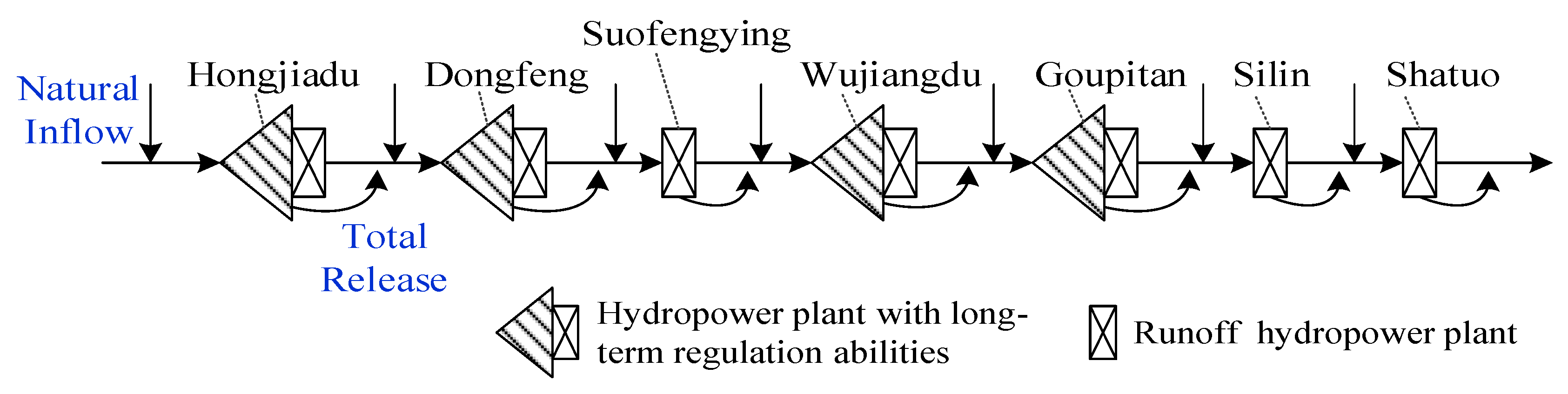
With extremely rich hydropower resources, many huge cascaded hydropower plants have been constructed in southwestern China. As the main sending end for the West-to-East Electricity Transmission (WEET) Project, these hydropower plants face a special multi-market environment. They not only have to supply the load for the local provincial market, but also need to deliver electricity to the central and eastern load centers in the external market [5], which has a direct impact on the supply and demand balance of the two markets and, as a result, the electricity prices of the two markets are closely correlated. Under such circumstances, optimizing the generation scheduling for cascades in different markets, improving the overall benefits, and coping with the market risks is a practical problem to be solved by the hydropower enterprises. However, this problem becomes much more complicated due to the uncertainty of electricity prices and the correlation of prices in different markets. In addition, the hydraulic and market constraints of the cascade hydropower plants increase the complexity further [6].

The generation scheduling for hydropower plants is a typical multi-variable and non-linear problem [7,8], especially for cascade hydropower plants. It has close internal cascade dependency, indicating that the water release from the upstream reservoir is the inflow of the downstream reservoir [9]. In the deregulated market, which is different from a conventional centralized operation, producers most important objectives are to generate power with more benefits [10,11] and lower market risks [12]. To get hydropower producers involved in the electricity market, scholars have carried out many studies and have made great achievements. The electricity price policies, such as the market clearing price (MCP), peak-valley price, time-of-use (TOU) price, and so on, are considered in the generation scheduling models of hydropower plants [13,14], as the electricity prices directly affect the market benefits. Accordingly, an uncertainty description of electricity prices is also proposed to improve the robustness of the models, in which the electricity prices are treated as variables rather than fixed constants [15,16,17]. At the same time, with the expansion of wind power, for photovoltaic power, and other distributed energy sources, the uncertainties in the power system have increased dramatically, and research on uncertainty-based models [18] and stochastic models [19] have drawn more and more attention. Corresponding to the hydropower generation scheduling models, some scholars have introduced market risk constraints to further improve the reliability of optimizing the trading strategies [20,21]. Overall, from the perspective of the time horizon, most existing studies focus on optimization in the daily market, and, as a result, the medium- and long-term studies are in a small quantity [22]. Price uncertainty has been included in the generation scheduling models, but it is mainly for a single market and the correlation of stochastic prices between multiple markets has not been considered. Despite the fact Under the background of fact that that hydropower plants in southwestern China challenge a new multi-market environment, a new generation scheduling model needs to be developed.

To solve the aforesaid problem and achieve a successful implementation for cascade hydropower plants in the multi-market environment, a novel long-term generation scheduling model for cascade hydropower plants is proposed. The main contributions are summarized as follows:

(1) The correlations of the MCP between different markets is described. The prediction price is treated as a random variable that consists of its prediction value and a random prediction error. The MCP scenarios for the multi-market environment are then generated by using the Copula theory, and are further reduced by the hierarchical clustering method combined with inconsistent values.

(2) A novel long-term generation scheduling model is constructed, based on the stochastic programming theory and the reduced MCP scenarios, in which the market-to-market supply energy ratio constraint and the minimum constraint of supply energy in the provincial market are creatively taken into consideration, so as to meet the actual engineering needs.

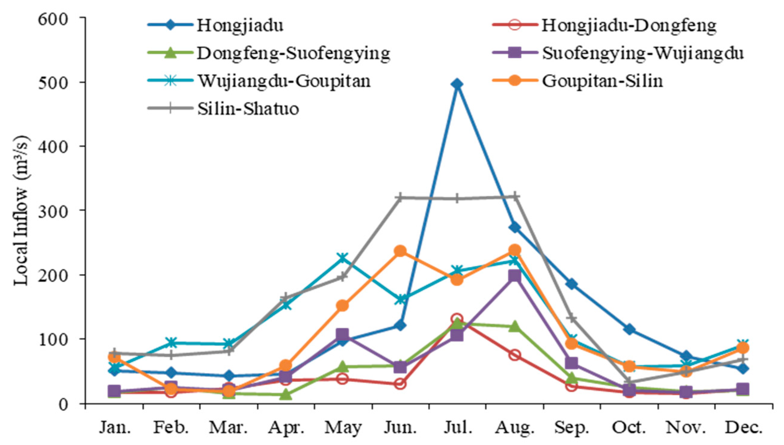
(3) The effectiveness and robustness of the proposed model have been validated by applying it to perform the long-term generation scheduling of the Wu River cascade hydropower plants in China. Compared with the conventional scheduling model, the proposed model can better respond to the MCP signals and gain the optimal trading strategy for different time periods and markets. It can also adapt to different MCP scenarios, and thus provides a theoretical reference for large-scale hydropower consumption in southwestern China under the new electricity market environment.

The remainder of this paper is organized as follows: In Section 2, the MCP scenarios for multiple markets are described. Section 3 is devoted to the detailed presentation of the proposed optimization model. In Section 4, the solution method for the proposed model is introduced. In Section 5, the case study and optimization results are carefully discussed. Finally, Section 6 outlines the main conclusions.

2. Description of MCP Scenarios for Multiple Markets

The market electricity price derives from a complex process with uncertain factors [23,24], and is generally obtained through prediction methods in the stage of reporting transactions [25]. However, the prediction price is subject to many factors, such as the accuracy of the input data and the fitting parameters, and there may be a certain prediction error, objectively. Directly using the deterministic prediction value will bring participants many more market risks. In this paper, the MCP is firstly described as a variable of its prediction value and random prediction error. Then, considering the correlation between the multiple markets, a joint distribution function of the MCP for the multi-market environment is constructed and further discretized into several independent and identical distribution scenarios. Finally, these scenarios are reduced based on the balance of the result’s accuracy and the computation workload.

2.1. Building MCP Scenarios Based on the Copula Theory

For any time period of $t$, the predicted MCP of market $i$ is denoted by ${\widehat{\lambda }}_{i,t}$, and the prediction error is ${\epsilon }_{i,t}$. The actual MCP ${\lambda }_{i,t}$ can be described as a random variable of ${\widehat{\lambda }}_{i,t}$ and ${\epsilon }_{i,t}$. That is:

$${\lambda }_{i,t}={\widehat{\lambda }}_{i,t}+{\epsilon }_{i,t}\left({\lambda }_{i,t}^{\min }\le {\lambda }_{i,t}\le {\lambda }_{i,t}^{\max }\right)$$

(1)

where, $i=1,2,\cdots ,I$ indicates the serial number of the market, and the total number of markets, $I$; ${\lambda }_{i,t}^{\max }$ and ${\lambda }_{i,t}^{\min }$, indicate the upper and lower bounds for ${\lambda }_{i,t}$, respectively.

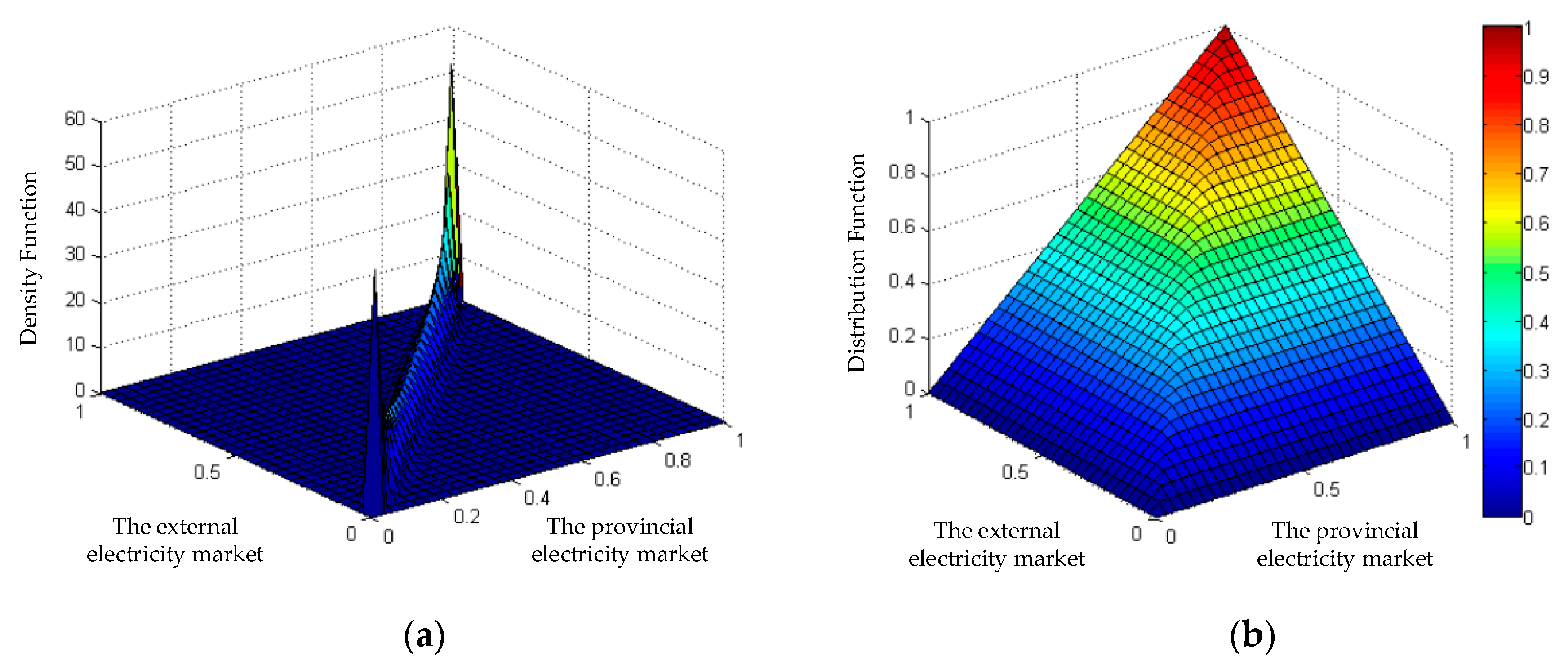
Due to the complex correlation between supply and demand of multiple markets, the MCPs of these markets can fluctuate greatly and are related to each other, thus the MCP of each market is not appropriate for separate description. In this paper, the Copula theory in econometrics is introduced to describe the correlation of MCPs in multiple markets, and a method for generating combined MCP scenarios (i.e., MCP scenarios for multi-markets) based on the Copula function is proposed. The Copula theory was firstly proposed by Sklar in 1959 to describe complex nonlinear correlations between random variables, which is now widely used in the financial sector as it has no restrictions on the marginal distribution of variables [26]. The Copula function can put the marginal distributions together to form a joint distribution, and its strict definition is given later by Nelsen [27]. That is, there is a function $C$ that makes:

$$H\left(x_1,x_2,\cdots ,x_n\right)=C\left(H_1\left(x_1\right),H_2\left(x_2\right),\cdots ,H_n\left(x_n\right)\right)$$

(2)

where, $H$ is the joint distribution function of the random vectors $x_1,x_2,\cdots ,x_n$, and its marginal distribution is $H_1\left(x_1\right),H_2\left(x_2\right),\cdots ,H_n\left(x_n\right)$, respectively. It has been proved that if all these marginal distributions are continuous, the Copula function $C$ is unique.

Defining $H_i^{-1}\left(x_i\right),i\in \{1,2,\cdots ,n\}$ as the inverse function of $H_i\left(x_i\right)$, the Copula function can be expressed as:

$$C\left(u_1,u_2,\cdots ,u_n\right)=H\left(H_1^{-1}\left(u_1\right),H_2^{-1}\left(u_2\right),\cdots ,H_n^{-1}\left(u_n\right)\right)$$

(3)

where, $u_i\left(i=1,2,\cdots ,n\right)$ is a variable obeying uniform distribution in $\left[0,1\right]$. Obviously, the Copula function $C\left(u_1,u_2,\cdots ,u_n\right)$ is a joint distribution function constructed by $n$ marginal distributions of uniform distribution in $\left[0,1\right]$. There are five commonly used Copula functions, including Gaussian-, t-, Gumbel-, Clayton- and Frank-Copula functions. Their expressions, characteristics, and density distribution plots are listed in

Table 1. The general information of five commonly used Copula functions.

Type	Expression	Characteristics	Density Distribution Plot
Gaussian	$\begin{array}{l}C\left(u_1,u_2;\rho \right)\\ ={\Phi }_{\rho }\left({\Phi }_{}^{-1}\left(u_1\right),{\Phi }_{}^{-1}\left(u_2\right)\right)\end{array}$	Distributed symmetrically, without reflecting the tail correlation
t	$C\left(u_1,u_2;\rho ,k\right)=t_{\rho ,k}\left(t_k^{-1}\left(u_1\right),t_k^{-1}\left(u_2\right)\right)$	Distributed symmetrically, reflecting the tail correlation
Gumbel	$\begin{array}{l}C\left(u_1,u_2;\alpha \right)\\ =\exp \left(-{\left[{\left(-\ln u_1\right)}^{\alpha }+{\left(-\ln u_2\right)}^{\alpha }\right]}^{\frac{1}{\alpha }}\right)\end{array}$	Distributed asymmetrically, the upper tail related and the lower tail independent
Clayton	$\begin{array}{l}C\left(u_1,u_2;\alpha \right)\\ =\max \left({\left[u_1^{-\alpha }+u_2^{-\alpha }-1\right]}^{\frac{1}{\alpha }},0\right)\end{array}$	Distributed asymmetrically, the upper tail independent and the lower tail related
Frank	$\begin{array}{l}C\left(u_1,u_2;\alpha \right)\\ =-\frac{1}{\alpha }\ln {\left(1+\frac{\left(e^{-\alpha u_1}-1\right)\left(e^{-\alpha u_2}-1\right)}{e^{-\alpha }-1}\right)}^{\frac{1}{\alpha }}\end{array}$	Distributed symmetrically, without reflecting the tail correlation

.

As mentioned above, the cascade hydropower plants in southwestern China mainly participate in two electricity markets, i.e., the provincial and external markets. Based on the Copula theory, the combined MCP scenarios were generated using the following steps:

(1) Construct MCP marginal cumulative distribution functions for the provincial and external markets. As the MCP ${\lambda }_{i,t}$ is related to its prediction value ${\widehat{\lambda }}_{i,t}$ and prediction error ${\epsilon }_{i,t}$, the distribution function for ${\epsilon }_{i,t}$ needs to be firstly determined. At the early stage of reform, the monthly MCP data were accumulated for a short time and the distribution of prediction error was not clear. Therefore, according to the central limit theorem, suppose that ${\epsilon }_{i,t}~N\left(0,{\sigma }_{i,t}^2\right)$, then ${\lambda }_{i,t}~N\left({\widehat{\lambda }}_{i,t},{\sigma }_{i,t}^2\right)$, namely, the MCP of market $i$ is subject to the Gaussian distribution with the mean value ${\widehat{\lambda }}_{i,t}$ and variance ${\sigma }_{i,t}$. The probability density function (PDF) is:

$$h\left({\lambda }_{i,t}\right)=\frac{1}{\sqrt{2\pi }{\sigma }_{i,t}}{e}^{-\frac{{\left({\lambda }_{i,t}-{\widehat{\lambda }}_{i,t}\right)}^2}{2{\sigma }_{i,t}^2}},{\lambda }_{i,t}^{\min }\le {\lambda }_{i,t}\le {\lambda }_{i,t}^{\max }$$

(4)

Then, the marginal cumulative distribution function H is obtained by the integral of $h\left({\lambda }_{i,t}\right)$. That is:

$$H_i\left({\lambda }_{i,t}\right)=P\left\{\xi \le {\lambda }_{i,t}\right\}={\displaystyle {\int }_{{\lambda }_{i,t}^{\min }}^{{\lambda }_{i,t}}h\left(s\right)ds}$$

(5)

(2) Identify parameters for the Copula function. According to the characteristics of marginal distribution functions, appropriate Copula functions were firstly selected, and the unknown parameter $\alpha$ was estimated by the maximum likelihood estimate method, and the estimated value is:

$$\widehat{\alpha }=\arg \max {\displaystyle \sum _{k=1}^K\ln c\left(H_1\left({\lambda }_{1,t}\right),H_2\left({\lambda }_{2,t}\right);\alpha \right)}$$

(6)

where, $c\left(H_1\left({\lambda }_{1,t}\right),H_2\left({\lambda }_{2,t}\right);\alpha \right)$ is the density function of the Copula function $C\left(u_1,u_2;\alpha \right)$.

(3) Check the fitting performance of the Copula function. The squared Euclidean distance $d^2$ is used and its expression is:

$$d^2={\displaystyle \sum _{i=1}^n{\left|C\left(u_{1,i},u_{2,i};\alpha \right)-G\left(u_{1,i},u_{2,i};\alpha \right)\right|}^2}$$

(7)

where, $n$ is the number of samples, $C\left(u_1,u_2;\alpha \right)$ is the Copula function, and $G\left(u_1,u_2;\alpha \right)$ is the empirical distribution function. The smaller the value is, the better the fitting performance is.

(4) Generate the combined MCP scenarios. $S\times I$ dimensional data samples were generated by means of uniform discretization. $S$ and $I$ indicate, respectively, the number of samples and random variables. For each sample $\left(u_1^s,u_2^s\right)$, its combined MCP scenario vector ${\xi }_s=\left({\lambda }_{1,t}^s,{\lambda }_{2,t}^s\right)$ could be obtained by the inverse operation of the marginal distribution function, i.e., ${\lambda }_{i,t}=H_i^{-1}\left(u_i\right)$, and the probability of the scenario is $P_r({\xi }_s)=1/S$.

2.2. Reducing MCP Scenarios

Generally, the results will be more accurate with more simulated scenarios, but the computation scale and time will increase accordingly. To guarantee the result accuracy and simultaneously strike a balance with the computing workload, the number of scenarios needed to be properly determined. Clustering is a commonly used scenario reduction method, but the number of reserved clusters is difficult to determine. In this paper, the hierarchical clustering method combined with inconsistent values is introduced to reduce the MCP scenarios, and the silhouette value was used to measure the rationality of clustering results. The process of reducing scenarios is detailed below:

(1) Take each MCP scenario as a cluster and calculate the distance between every two clusters. Then, the absolute distance is adopted.

(2) Merge the nearest two clusters into a new cluster and calculate the distance between the new cluster and other clusters.

(3) Repeat steps (1) and (2) until all MCP scenarios are merged together.

(4) Calculate the inconsistent values after each merging and express them as $\left\{{\theta }_k,k=1,2,\cdots ,S-1\right\}$, and

$${\theta }_k=\frac{d_k-{\overline{d}}_k}{{\sigma }_k}$$

(8)

where, ${\theta }_k$ is the inconsistent value after the $k$th merging. $S$ is the number of total original scenarios, $d_k$ is the distance between the two clusters of the $k$th merging, ${\overline{d}}_k$ is the mean value of the distances calculated in the $k$th merging, and ${\sigma }_k$ is the standard deviation of the distances calculated in the $k$th merging. The inconsistent value was calculated by the inconsistent function in MATLAB. Each inconsistent value was a measure of separation between the two merged clusters, compared to the separation between subclusters merged within those clusters. If only two original MCP scenarios are merged in the $k$th merging, the inconsistent value is 0. Defining $\Delta {\theta }_k={\theta }_k-{\theta }_{k-1}$, the larger the $\Delta {\theta }_k$ was, the worse clustering result of the $k$th merging was, and the better the clustering result of the $k-1$th merging was.

Generally, the larger the number of reserved clusters, the more the reserved scenarios remain consistent with the original MCP scenarios, and the computation time will increase accordingly. The final number of reserved clusters could be determined by reference to the variation of inconsistent values $\left\{{\theta }_k,k=1,2,\cdots ,S-1\right\}$.

(5) The silhouette value proposed by Rousseeuw [28] is often used to evaluate the result of the cluster analysis, which can be calculated by Equation (9):

$${\beta }_i=\frac{b_i-a_i}{\max \left(a_i,b_i\right)}$$

(9)

where, ${\beta }_i$ is the silhouette value of scenario $i$, $i=1,2,\cdots ,S$, $r$ is the cluster index that scenario $i$ belongs to, $a_i$ is the average distance between scenario $i$ and other scenarios in the cluster $r$, and $b_i=\min \left(b_{i,1},\cdots ,b_{i,l},\cdots ,b_{i,R}\right)$, $b_{i,l}$ is the average distance between scenario $i$ and all scenarios in the cluster $l$, $l\ne r$. The range of ${\beta }_i$ is $\left[-1,1\right]$, and the larger the ${\beta }_i$, the better the clustering result of scenario $i$.

(6) Define the number of reserved clusters as $S^{\prime }$. For cluster $s\left(1\le s\le S^{\prime }\right)$, the representative scenario is ${\xi }^s$, and can be calculated as below:

$$\{\begin{array}{l}{\Omega }_s=\left\{{\xi }^{s,1},\cdots ,{\xi }^{s,m},\cdots ,{\xi }^{s,M}\right\}\\ {\xi }^{s,m}=\left\{{\lambda }_{1,t}^{s,m},\cdots ,{\lambda }_{i,t}^{s,m},\cdots ,{\lambda }_{N,t}^{s,m}\right\}\\ {\lambda }_{i,t}^s=\frac{1}{M}{\displaystyle \sum _{m=1}^M{\lambda }_{i,t}^{s,m}}\\ {\xi }^s=\left\{{\lambda }_{1,t}^s,\cdots ,{\lambda }_{i,t}^s,\cdots ,{\lambda }_{N,t}^s\right\}\end{array}$$

(10)

The occurrence probability of scenario ${\xi }^s$ is derived from Equation (11):

$$P_{r,t}\left({\xi }_s\right)=\frac{M}{S}$$

(11)

where, ${\Omega }_s$ is the set of scenarios involved in cluster $s$, ${\xi }^{s,m}$ is the scenario $m$ involved in cluster $s$, ${\lambda }_{1,t}^{s,m}$ is the electricity price of market $i$ in period $t$ under scenario $m$, ${\lambda }_{i,t}^s$ is the electricity price of market $i$ in period $t$ under representative scenario ${\xi }^s$, $m$ is the scenario index involved in cluster $s$, $1\le m\le M$, $t$ is the time period, $1\le t\le T$, $i$ is the market index, $1\le i\le N$, and $N$ is the total number of sub markets for the participation of hydropower cascades.

3. Optimization Model

In this paper, the cascade hydropower plants are assumed as one generator in the electricity market and cleared by the MCP. The annual market is considered and each time period represents one month. The operation objective was to maximize the market benefits. Considering the different MCP scenarios in the future period, the objective function can be defined as Equation (12).

$$\max B={\displaystyle \sum _{t=1}^T\left[{\displaystyle \sum _{s=1}^{{S^{\prime }}_t}\left(e_{1,t}^s{\lambda }_{1,t}^s+e_{2,t}^s{\lambda }_{2,t}^s\right)\times P_{r,t}\left({\xi }_s\right)}\right]}$$

(12)

where, $e_{i,t}^s$ is the supply energy for market $i$ in the time period $t$ under the representative scenario ${\xi }^s$, ${S^{\prime }}_t$ is the number of reserved scenarios in period $t$. The hydropower generation cost mainly involved the constant cost with little influence on the optimization results, and so it was not considered in the optimization model. For the cascade hydropower plants in southwestern China, the provincial and external markets are considered, $i=1$ for the provincial market and $i=2$ for the external market.

To get the proposed model more applicable to the scheduling in practice, the energy ratio for different electricity markets and the minimum supply energy for the provincial market, during the whole scheduling period, were also included in the constraints. The constraints involved in the model were as follows, in which the hydraulic constraints also can be seen in [8,9,13].

(1) Water balance equation:

$$\{\begin{array}{l}{V}_{m,t+1}=V_{m,t}+(Q_{m,t}-q_{m,t}-d_{m,t})\Delta T_t\\ Q_{m,t}=q_{m-1,t}+d_{m-1,t}+I_{m,t}\end{array}$$

(13)

where, $V_{m,t}$ and $V_{m,t+1}$ are the storage of reservoir $m$ at the beginning and end of the time period $t$, respectively, m³; $Q_{m,t}$ is the total inflow of reservoir $m$ in the period $t$, $q_{m,t}$, $d_{m,t}$, and $I_{m,t}$ are the power release, non-power release, and natural inflow of reservoir $m$ in the time period $t$, respectively, m³/s, $m=1,2,\cdots ,M$ is the reservoir index, $m-1$ is the index of the upstream reservoir of reservoir $m$, and $\Delta T_t$ is the number of seconds in the period $t$.

(2) Initial and end reservoir level constraints:

$$Z_{m,1}={Z^{\prime }}_{m,1}\forall m\in M$$

(14)

$$Z_{m,T}={Z^{\prime }}_{m,T}\forall m\in M$$

(15)

where, ${Z^{\prime }}_{m,1}$ and ${Z^{\prime }}_{m,T}$ are the initial and end reservoir levels of planning horizon, respectively, which are specified before the optimization process, m. In the case study, ${Z^{\prime }}_{m,1}$ and ${Z^{\prime }}_{m,T}$ were specified based on the historical records for practical operation.

(3) Outflow constraint:

$${\underset{\_}{q}}_{m,t}\le q_{m,t}\le {\overline{q}}_{m,t}$$

(16)

where, ${\underset{\_}{q}}_{m,t}$ and ${\overline{q}}_{m,t}$ are the minimum and maximum outflow of plant $m$ in the time period $t$, m³/s.

(4) Power generation constraint:

$${\underset{\_}{p}}_{m,t}\le p_{m,t}\le {\overline{p}}_{m,t}$$

(17)

where, ${\underset{\_}{p}}_{m,t}$ and ${\overline{p}}_{m,t}$ are the minimum and maximum power generation of plant $m$ in the time period $t$, MW.

(5) Storage boundary constraint:

$${\underset{\_}{V}}_{m,t}\le V_{m,t}\le {\overline{V}}_{m,t}$$

(18)

where, ${\underset{\_}{V}}_{m,t}$ and ${\overline{V}}_{m,t}$ are the minimum and maximum storage for reservoir $m$ at the beginning of the time period $t$, respectively, m³.

(6) Market-to-market energy ratio constraint:

$$\{\begin{array}{l}\raisebox{1ex}{$E_1$}\!\left/ \!\raisebox{-1ex}{$E_2$}\right.=\theta \\ E_1={\displaystyle \sum _{t=1}^T{e}_{1,t}}\\ E_2={\displaystyle \sum _{t=1}^T{e}_{2,t}}\end{array}$$

(19)

where, $\theta$ is the energy ratio of cascade hydropower plants involved in the provincial and external markets, which is agreed by the power producers in the river basin, the provincial development and reform commission, and other parties, $e_{i,t}$ is the supply energy of cascade hydropower plants for market $i$ in the time period $t$, MWh, and $E_1$ and $E_2$ are the supply energy of cascade hydropower plants in the provincial and external markets, respectively, during the whole optimization horizon, MWh.

(7) Minimum supply energy for provincial market:

$$e_{1,t}\ge e_{1,t}^{\min }$$

(20)

where, $e_{1,t}^{\min }$ is the minimum supply energy of the cascade hydropower plants in the provincial market in period $t$, MWh.

(8) Relationship between fore-bay water level and reservoir storage:

$$Z_{m,t}=a_{0,m}+a_{1,m}{V}_{m,t}+a_{2,m}{V}_{m,t}^2+a_{3,m}{V}_{m,t}^3+a_{4,m}{V}_{m,t}^4$$

(21)

where, $Z_{m,t}$ is the fore-bay water level for reservoir $m$ in period $t$, m $V_{m,t}$ is the storage for reservoir $m$ in the period $t$, m³, and the coefficients $\left(a_{i,m},i=1,2,3,4\right)$ are fitting parameters for reservoir $m$.

(9) Relationship between tailrace level and total release:

$$Z{T}_{m,t}=b_{0,m}+b_{1,m}{R}_{m,t}+b_{2,m}{R}_{m,t}^2+b_{3,m}{R}_{m,t}^3+b_{4,m}{R}_{m,t}^4$$

(22)

where, $Z{T}_{m,t}$ is the tailrace level for reservoir $m$ in the time period $t$, m, and the coefficients $\left(b_{i,m},i=1,2,3,4\right)$ are fitting parameters for reservoir $m$.

(10) Generation of cascade power plants:

$$e_{1,t}+e_{2,t}={\displaystyle \sum _{m=1}^M{A}_{m,t}{q}_{m,t}{H}_{m,t}}\Delta T_t$$

(23)

where, $A_{m,t}$ and $H_{m,t}$ are the generation efficiency coefficient and water head of plant $m$ in the time period $t$, respectively, and $H_{m,t}=\frac{Z_{m,t}+Z_{m,t+1}}{2}-Z{T}_{m,t}$.

4. Solution Method

The solution method typically depends on the characteristics of the optimization model. The commonly used solution methods for cascaded hydropower plants fall into three categories: Mathematical programming, dynamic programming and its improved algorithms, and artificial intelligence algorithms. The aforesaid optimization problem, including Equation (19), Equation (21), Equation (22), and other nonlinear constraints, is a typical nonlinear problem. Especially, the proposed model cannot meet the Markovian character, because the market-to-market energy ratio constraint, i.e., constraint (6), is included. Consequently, the dynamic programming and similar algorithms are not applicable. Moreover, the intelligent algorithms have problems, such as long computing time, easily trapped into local optimization, and unstable calculation results. Therefore, nonlinear programming (NLP) in mathematical programming is chosen in this paper.

In this paper, the solution procedure involves two main steps. At step 1, the combined MCP scenarios are generated and reduced by using MATLAB software; at step 2, based on the reduced scenarios, the NLP is implemented by the Global Solver, available in LINGO 17.0 (http://www.lindo.com/), to solve the proposed model. LINGO is a special software for solving mathematical programming problems, such as linear programming, non-linear programming, quadratic programming, and integer programming problems. It has the advantages of easy operation, fast computation, and stable calculation results. The basic computational principle and detailed computational procedure of the Global Solver for solving NLP problems have been given in literatures [29,30]. It mainly includes three steps: (1) With the branch-and-bound algorithm, the entire feasible solution spaces are segmented into series sub-problems; (2) a slack problem for each sub-problem can be obtained by convexity and linearization transformation and solved by the linear programming method; and (3) the global optimal solution is obtained by traversing all the sub-problems (i.e., the whole feasible space). Figure 1 shows the detailed calculating process. To set the parameters and calibrate the Global Solver, read the manual provided in LINDO.

5. Case Study

5.1. Study System

The proposed model was applied to the cascade hydropower plants of the Wu River in the Guizhou Province, China. Seven hydropower plants have been built on the mainstream of the Wu River, with a total installed capacity of 8345 MW. Figure 2 shows the distribution chart of the Wu River cascade, with reservoir characteristics in

Table 2. Characteristics of the studied hydropower plants on the Wu River.

Plant Name	Installed Capacity (MW)	Normal Level (m)	Dead Level (m)	Regulation Coefficient	Maximum Power Release (m3/s)	Generation Efficiency (kW/(m3/s)/m)
Hongjiadu	600	1140	1076	0.72	490.5	8.50
Dongfeng	695	970	936	0.05	632.1	8.35
Suofengying	600	837	822	--	994.5	8.50
Wujiangdu	1280	760	720	0.09	1087.0	8.30
Goupitan	3000	630	590	0.14	1909.0	8.50
Silin	1050	440	431	--	1772.8	8.50
Shatuo	1120	365	353.5	--	1969.2	8.50

Note: The regulation coefficient could be calculated from the division of the beneficial storage by the average inflow water volume.

. Four hydropower plants have long-term regulation abilities in the studied cascade, and they are Hongjiadu, Dongfeng, Wujiangdu, and Goupitan. The storage capacities of the other three reservoirs were much smaller, and they were addressed as runoff hydropower plants in the long-term operation. Thus, the cascade power decisions were distributed through the operation of these four large reservoirs. In this paper, the long-term provincial and external electricity markets are considered, assuming that the energy ratio between the markets is 3:1. The estimated electricity MCP and the standard deviation of estimated error are treated as known and given in

Table 3. The parameters of market clearing price (MCP) for market 1, 2 in a different month (yuan/MWh).

Month	Market 1		Market 2		Month	Market 1		Market 2
	$\widehat{\mathit{\lambda }}$	$\mathit{\sigma }$	$\widehat{\mathit{\lambda }}$	$\mathit{\sigma }$		$\widehat{\mathit{\lambda }}$	$\mathit{\sigma }$	$\widehat{\mathit{\lambda }}$	$\mathit{\sigma }$
Jan.	311.56	15.58	303.30	15.17	Jul.	265.11	13.26	298.42	14.92
Feb.	325.32	16.27	322.68	16.13	Aug.	266.79	13.34	300.76	15.04
Mar.	316.65	15.83	300.83	15.04	Sep.	246.27	12.31	246.43	12.32
Apr.	293.86	14.69	300.93	15.05	Oct.	255.16	12.76	290.43	14.52
May	287.12	14.36	283.43	14.17	Nov.	288.58	14.43	261.76	13.09
Jun.	283.23	14.16	279.26	13.96	Dec.	316.87	15.84	258.71	12.94

Note: $\widehat{\lambda }$ indicates the estimated electricity MCP; $\sigma$ indicates the standard deviation of the estimated error.

. The monthly local inflow data in 2016 were used for simulation and shown in Figure 3. In the later text, market 1 represents the provincial electricity market and market 2 represents the external electricity market. All the basic data of the study system was collected from the dispatching center of the Wu River basin.

5.2. Results Discussion

5.2.1. Scenarios Analysis

The Copula function should be adopted to fit the MCPs in the provincial and external markets. In this paper, it is assumed that the prediction error is the Gaussian distribution with the mean value of 0. Therefore, the probability density distribution was symmetric for the MCPs in the provincial and external markets. Three symmetrically distributed Copula functions in Table 1, including the bivariate Gaussian-Copula function, bivariate t-Copula function and bivariate Frank-Copula function were candidate functions, but the final closed function should be subject to the fitting performance.

There were 1000 groups of samples generated discretely. Based on the marginal distribution functions of MCPs in the provincial and external markets, the parameter estimation result of different Copula functions is shown in

Table 4. Parameter estimation of different Copula functions.

Month	Gaussian	t		Frank	Month	Gaussian	t		Frank
	$\mathit{\rho }$	$\mathit{\rho }$	$\mathit{k}$	$\mathit{\alpha }$		$\mathit{\rho }$	$\mathit{\rho }$	$\mathit{k}$	$\mathit{\alpha }$
Jan.	0.9987	0.8764	8.5060	13.3732	Jul.	0.9866	0.8659	8.2926	7.9900
Feb.	0.9994	0.9868	7.4947	44.0535	Aug.	0.9807	0.8264	8.3761	7.9351
Mar.	0.9883	0.8756	5.9924	7.1498	Sep.	0.9999	0.9985	8.4007	8.9437
Apr.	0.9949	0.8996	7.3280	15.1018	Oct.	0.9862	0.9221	5.2463	9.6618
May	0.9868	0.9674	7.2697	27.6052	Nov.	0.9942	0.9441	12.9855	8.7701
Jun.	0.9829	0.9615	7.3714	25.5160	Dec.	0.9838	0.9138	9.4283	8.1087

. The fitting performance of different Copula functions is tested by Equation (7), and the result is shown in

Table 5. The fitting performance results of different Copula functions.

Copula	Jan.	Feb.	Mar.	Apr.	May	Jun.	Jul.	Aug.	Sep.	Oct.	Nov.	Dec.
Gaussian-	0.0035	0.0089	0.0543	0.0294	0.0597	0.0736	0.0605	0.0813	0.0052	0.0619	0.0322	0.0704
t-	0.4155	0.0586	0.4136	0.3402	0.1240	0.1433	0.4471	0.5714	0.0136	0.2670	0.2012	0.2968
Frank-	0.2631	0.0414	0.6750	0.2168	0.0833	0.0942	0.5773	0.5830	0.4896	0.4361	0.5040	0.5652

. It can be seen that the values of the Gaussian-Copula function were the smallest, which indicates the better fitting performance of the Gaussian-Copula function in each month compared with the t- and Frank-Copula functions. Therefore, the Gaussian-Copula function was used to describe the correlation between the MCPs in the provincial and external markets. Taking April as an example, the Gaussian-Copula density and distribution function are shown in Figure 4.

It is well known that the more discrete scenarios are, the more precise the description of the original distribution will be. However, the typicality of each scenario will be poor, and the workload for computation will be more. Upon the test, there are 1000 sets of scenarios generated by monthly discretization. After scenario reduction, the minimum number of scenarios from January to December is 47, and the maximum number is 64. A diagram of silhouette values is shown in Figure 5. It was found that the silhouette values were positive for each original scenario after clustering, and more than 95% silhouette values were greater than 0.2 for the original scenarios. This indicated that the classification number determined by the inconsistent values was appropriate, and the scenario set after clustering could be used to describe the original scenario set.

5.2.2. Effectiveness Analysis

The effectiveness of the proposed model was verified by the comparison with the conventional model. In the conventional model, the electricity price factor was not included, but only to achieve the maximum expected power generation in the scheduling horizon, maintain an adequate security of supply, and arrange the cascade plants to deliver electricity outwards in a certain proportion in case of spilled water in the flood seasons. In 2016, the natural inflow concentrated from June to August, accounted for 50% of the total inflow in the year. There was a risk of spilled water, and so the cascade hydropower plants were arranged to deliver electricity outwards, i.e., participate the external electricity market. Other constraints, such as the final water level, maximum and minimum power output, combined MCP scenarios, and so on, were the same for the two models.

Figure 6 shows the water level of the cascade hydropower plants with regulation capacity, and the power output process were also obtained. It was found that the water level change trend of each hydropower plant was consistent for both the proposed model and conventional model. Generally, before the flood seasons, the water level of each hydropower plant fell, vacating the reservoir. During the flood seasons, the water was stored, the water level rose, and the generation water head increased. After the flood seasons, the water level reduced back to the control water level. These trends were in line with the cascade hydropower operation rules.

In terms of power generation in different months, the power generation of the proposed model during the dry seasons was much more than the conventional model, and the water level drops of each hydropower plant before the flood seasons were greater. This was because the power market was of a high proportion of hydropower and price in dry seasons was much higher. The hydropower plants with regulation ability preferred to use a self-regulating storage capacity to achieve the redistribution of water, so as to respond to price changes and improve their benefits. For example, in the proposed model, the water level drop at the Hogjiadu plant (i.e., the first stage of the cascade plants) was serious before the flood seasons, and it was close to the lowest operation water level. When the flood seasons came, the Hongjiadu plant was concentrated to store water and almost no power was generated. The water level of the downstream plants, including Dongfeng, Wujiangdu, and Goupitan, changed lightly between the flood seasons and dry seasons, which, to some extent, benefitted from inflow compensation of the Hongjiadu plant. Therefore, these downstream hydropower plants could keep a high water head for high generation efficiency.

Figure 7 shows the supply energy for the two different markets obtained by the two comparison models under the assumptions that the same MCP scenarios were adopted. According to the analysis, on the basis of ensuring the power supply in the province market during the scheduling horizon, the proposed model responded better to the changing of market electricity prices and arranged the electricity delivery plan rationally. The power generation in the dispatching periods was 23.98 billion kWh, and the power generation revenue was 7.11 billion yuan. They were 24.07 billion kWh and 7.00 billion yuan, respectively, for the conventional model. It was found that, based on the same energy storage at the end of scheduling period, the proposed model resulted in an increase of 106.93 million yuan for the total income, although the power generation was less, compared with the conventional model. This proved that the electricity price factors would greatly influence the expected benefits in the market of the cascade hydropower plants.

5.2.3. Robustness Analysis

The robustness of the proposed model was verified by the comparison with different price scenarios. Five typical MCP scenarios were selected for the comparison. Scenario 1 embodied the situation for good prediction, and actual electricity price was higher than the prediction value. Scenario 2 embodied the situation for good prediction and the actual electricity price was lower than the prediction value. Scenario 3 embodied the situation for perfect prediction and the actual electricity price was exactly the same as the prediction value. Scenario 4 embodied the situation for poor prediction and the actual electricity price was higher than the prediction value. Scenario 5 embodied the situation for poor prediction and the actual electricity price was lower than the prediction value. For different scenarios, the indicators for evaluating the prediction result, including the mean absolute percent error (MAPE), the mean average error (MAE) and the relative correlation coefficient (R), are listed in

Table 6. The detailed information of different scenarios.

Scenario	MAPE (%)	MAE (yuan/MWh)	R	Prediction Performance
1	1.92	5.65	0.9560	good
2	2.00	5.81	0.9609	good
3	0	0	0	perfect
4	13.02	37.33	0.5590	poor
5	12.27	34.90	0.5113	poor

.

The comparison results are shown in

Table 7. Operation results comparison of multi scenarios (Unit: Billion yuan).

Scenario	Benefit of Proposed Model			Benefit of Conventional Model
	Market 1	Market 2	Total	Market 1	Market 2	Total
1	5.369	1.813	7.182	6.250	0.788	7.039
2	5.268	1.744	7.013	6.119	0.759	6.878
3	5.353	1.791	7.144	6.229	0.779	7.008
4	5.467	1.668	7.135	6.163	0.796	6.959
5	5.293	1.668	6.961	6.032	0.795	6.827
Probability combination	5.318	1.793	7.110	6.224	0.780	7.003

. It was found that the benefits of other MCP scenarios were in the range of Scenario 1 and Scenario 5 for both models. Compared with the conventional model, the proposed model achieved better power generation benefits in different MCP scenarios. Even in the adverse scenario with a serious deviation in the price prediction, the proposed model still had relatively higher benefits. For instance, in Scenarios 4 and 5, the benefits were 7.135 billion yuan and 6.961 billion yuan for the proposed model. However, they were 6.959 billion yuan and 6.827 billion yuan for the conventional model, decreased by 176.022 million yuan and 132.952 million yuan, respectively. This indicated that the proposed model could better adapt to different price scenarios in the future, and could enhance the profitability and robustness for the generation scheduling.

6. Conclusions

The large-scale cascade hydropower plants in southwestern China challenge a new multi- market environment. Considering the price uncertainty and the correlations between multiple markets, this paper has proposed a novel optimization model of long-term generation scheduling for cascade hydropower plants to seek for the overall benefits. The main contributions and conclusions were as follows:

(1) The correlation of MCP between multiple markets was described. The prediction price was treated as a random variable that consists of its prediction value and a random prediction error. Then, the MCP scenarios for the hybrid market environment were generated by using the Copula theory and further reduced by the hierarchical clustering method combined with inconsistent values.

(2) A novel long-term generation scheduling model was constructed based on the stochastic programming theory and the reduced MCP scenarios, in which the market-to-market supply energy ratio constraint and the minimum constraint of supply energy in the provincial market were creatively taken into consideration, so as to meet the actual engineering needs.

(3) The scenarios analysis showed that the Gaussian-Copula function has better fitting performance in describing the correlation between the MCPs of the provincial and external markets than other functions. The proposed reduction strategy for the MCP scenarios was effective, after the reduction of scenarios. The minimum number of scenarios from January to December was 47, and the maximum number was 64.

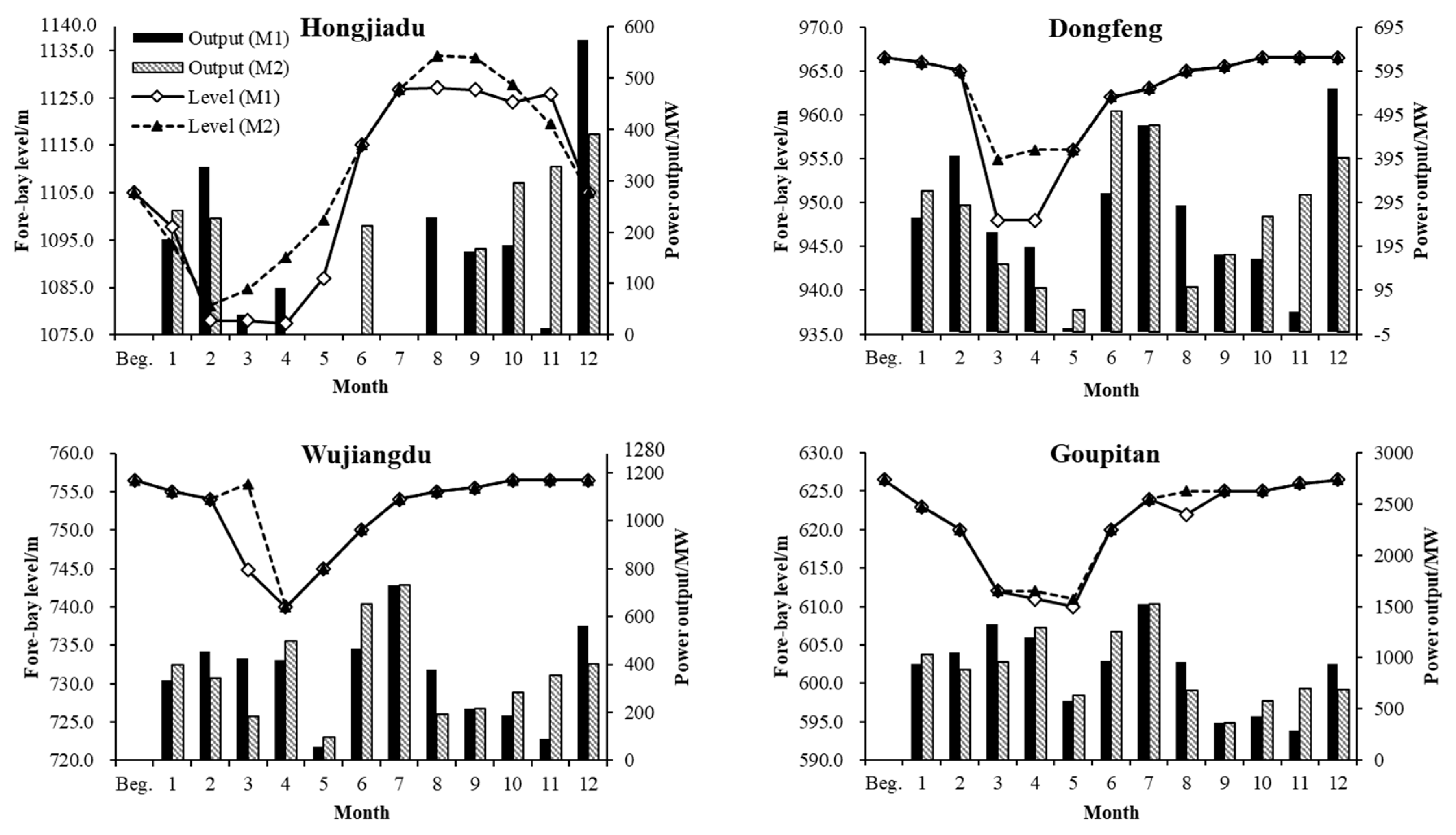
(4) The effectiveness analysis showed that the proposed model could better respond to the changing of MCP signals, and so the arrangement of power generation in different months and markets was more reasonable. This resulted in an increase of 106.93 million yuan for the total income, although the power generation was less, compared with the conventional model.

(5) The robustness analysis showed that the proposed model could better adapt to different price scenarios in the future, even in the adverse scenario, with a serious deviation in the price prediction. This enhanced profitability and robustness for the generation scheduling.

It should be mentioned that the market reform in China is still at an early stage and the available samples are in a relatively small quantity. This paper only analyzed qualitatively the price correlation between the provincial and external markets but did not give the specific influence factors and their different roles. With continuous accumulation of data in the future, the interaction characteristics between the markets, consumers, and producers can be analyzed in detail, so as to better describe the price correlation between multiple markets.

References

1. Wang, F.; Xu, H.; Xu, T.; Li, K.; Shafie-Khah, M.; Catalão, J.P. The values of market-based demand response on improving power system reliability under extreme circumstances. Appl. Energy 2017, 193, 220–231. [Google Scholar] [CrossRef]
2. Zhao, X.; Lyon, T.P.; Song, C. Lurching towards markets for power: China’s electricity policy 1985–2007. Appl. Energy 2012, 94, 148–155. [Google Scholar] [CrossRef]
3. Chen, F.; Liu, B.; Cheng, C.; Mirchi, A. Simulation and regulation of market operation in hydro-dominated environment: The Yunnan case. Water 2017, 9, 623. [Google Scholar] [CrossRef]
4. Zeng, M.; Yang, Y.; Wang, L.; Sun, J. The power industry reform in China 2015: Policies, evaluations and solutions. Renew. Sustain. Energy Rev. 2016, 57, 94–110. [Google Scholar] [CrossRef]
5. Cheng, C.; Yan, L.; Mirchi, A.; Madani, K. China’s booming hydropower: Systems modeling challenges and opportunities. J. Water Resour. Plann. Manag. 2016, 143, 02516002. [Google Scholar] [CrossRef]
6. Xu, B.; Zhong, P.A.; Du, B.; Chen, J.; Liu, W.; Li, J.; Guo, L.; Zhao, Y. Analysis of a stochastic programming model for optimal hydropower system operation under a deregulated electricity market by considering forecasting uncertainty. Water 2018, 10, 885. [Google Scholar] [CrossRef]
7. Cheng, C.; Shen, J.; Wu, X.; Chau, K. Operation challenges for fast-growing China’s hydropower systems and respondence to energy saving and emission reduction. Renew. Sustain. Energy Rev. 2012, 16, 2386–2393. [Google Scholar] [CrossRef]
8. Wen, X.; Zhou, J.; He, Z.; Wang, C. Long-term scheduling of large-scale cascade hydropower stations using improved differential evolution algorithm. Water 2018, 10, 383. [Google Scholar] [CrossRef]
9. Wu, X.; Cheng, C.; Zeng, Y.; Lund, J.R. Centralized versus distributed cooperative operating rules for multiple cascaded hydropower reservoirs. J. Water Resour. Plann. Manag. 2016, 142, 05016008. [Google Scholar] [CrossRef]
10. Gross, G.; Finlay, D. Generation supply bidding in perfectly competitive electricity markets. Comput. Math. Organ. Theory 2000, 6, 83–98. [Google Scholar] [CrossRef]
11. Bakirtzis, G.A.; Simoglou, C.; Ziogos, P.N.; Tellidou, C.A.; Bakirtzis, A.G. Electricity producer offering strategies in day-ahead energy markets. IEEE Trans. Power Syst. 2007, 22, 1804–1818. [Google Scholar] [CrossRef]
12. Liu, H.L.; Jiang, C.W.; Zhang, Y. A review on risk-constrained hydropower scheduling in deregulated power market. Renew. Sustain. Energy Rev. 2008, 12, 1465–1475. [Google Scholar]
13. Zhang, J.R.; Li, W.; Chen, Y.; Li, J.P. Modeling for cascaded reservoirs scheduling considering policy factors. In Proceedings of the 2009 International Joint Conference on Computational Sciences and Optimization, Sanya, China, 24–26 April 2009; Volume 2, pp. 447–451. [Google Scholar]
14. Pérez-Díaz, J.I.; Wilhelmi, J.R.; Sánchez-Fernández, J.Á. Short-term operation scheduling of a hydropower plant in the day-ahead electricity market. Electr. Power Sys. Res. 2010, 80, 1535–1542. [Google Scholar] [CrossRef]
15. Flatabø, N.; Haugstad, A.; Mo, B.; Fosso, O.B. Short-term and medium-term generation scheduling in the Norwegian hydro system under a competitive power market structure. In Proceedings of the International Conference on Electrical Power System Operation and Management, Zurich, Switzerland, 23–25 September 1998. [Google Scholar]
16. Mo, B.; Gjelsvik, A.; Grundt, A.; Karesen, K. Optimisation of hydropower operation in a liberalised market with focus on price modelling. In Proceedings of the IEEE Porto Power Tech Proceedings, Porto, Portugal, 10–13 September 2001. [Google Scholar]
17. De Ladurantaye, D.; Gendreau, M.; Potvin, J.Y. Strategic bidding for price-taker hydroelectricity producers. IEEE Trans. Power Syst. 2007, 22, 2187–2203. [Google Scholar] [CrossRef]
18. Najafi, A.; Marzband, M.; Mohamadi-Ivatloo, B.; Contreras, J.; Pourakbari-Kasmaei, M.; Lehtonen, M.; Godina, R. Uncertainty-based models for optimal management of energy hubs considering demand response. Energies 2019, 12, 1413. [Google Scholar] [CrossRef]
19. Home-Ortiz, J.M.; Melgar-Dominguez, O.D.; Pourakbari-Kasmaei, M.; Roberto, J.; Mantovani, S. A stochastic mixed-integer convex programming model for long-term distribution system expansion planning considering greenhouse gas emission mitigation. Int. J. Electr. Power Energy Syst. 2019, 108, 86–95. [Google Scholar] [CrossRef]
20. García-González, J.; Parrilla, E.; Mateo, A. Risk-averse profit-based optimal scheduling of a hydro-chain in the day-ahead electricity market. Eur. J. Oper. Res. 2007, 181, 1354–1369. [Google Scholar] [CrossRef]
21. Ilak, P.; Krajcar, S.; Rajšl, I.; Delimar, M. Pricing energy and ancillary services in a day-ahead market for a price-taker hydro generating company using a risk-constrained approach. Energies 2014, 7, 2317–2342. [Google Scholar] [CrossRef]
22. Flach, B.C.; Barroso, L.A.; Pereira, M.V.F. Long-term optimal allocation of hydro generation for a price-maker company in a competitive market: Latest developments and a stochastic dual dynamic programming approach. IET Gener. Transm. Distrib. 2010, 4, 299–314. [Google Scholar] [CrossRef]
23. Azadeh, A.; Moghaddam, M.; Mahdi, M.; Seyedmahmoudi, S.H. Optimum long-term electricity price forecasting in noisy and complex environments. Energy Sourcespart. B Econ. Plan. Policy 2013, 8, 10. [Google Scholar] [CrossRef]
24. Cheng, C.; Luo, B.; Miao, S.; Wu, X. Mid-term electricity market clearing price forecasting with sparse data: A Case in newly-reformed Yunnan electricity market. Energies 2016, 9, 804. [Google Scholar] [CrossRef]
25. Chen, J.; Garcia, H.E. Economic optimization of operations for hybrid energy systems under variable markets. Appl. Energy 2016, 177, 11–24. [Google Scholar] [CrossRef] [Green Version]
26. Makridakis, S.G.; Wheelwright, S.C. An analysis of the interrelationships among major world stock exchanges. J. Bus. Financ. Account. 1974, 1, 195–215. [Google Scholar] [CrossRef]
27. Nelsen, R.B. An Introduction to Copulas; Springer Publishing Company: Berlin/Heidelberg, Germany, 2006. [Google Scholar]
28. Rousseeuw, P.J. Silhouettes: A graphical aid to the interpretation and validation of cluster analysis. J. Comput. Appl. Math. 1987, 20, 53–65. [Google Scholar] [CrossRef] [Green Version]
29. Wang, J.; Cheng, C.; Shen, J.; Wu, X.; Cao, R. A branch-and-bound based global optimization method for deterministic hydropower operation. Proc. CSEE 2018, 38, 5107–5116. [Google Scholar]
30. Gau, C.Y.; Schrage, L.E. Implementation and Testing of a Branch-And-Bound Based Method for Deterministic Global Optimization: Operations Research Applications; Frontiers in Global Optimization; Springer: Boston, MA, USA, 2004; pp. 145–164. [Google Scholar]
Figure 1. The flow chart for calculation.
Energies 12 02239 g001
Figure 2. The distribution chart of the Wu River cascade.
Energies 12 02239 g002
Figure 3. The monthly local inflow of each reservoir in 2016.
Energies 12 02239 g003
Figure 4. The density and distribution function of Gaussian-Copula in April (p = 0.9949). (a) Density Function; (b) Distribution Function.
Energies 12 02239 g004
Figure 5. The diagram of silhouette values in each month.
Energies 12 02239 g005aEnergies 12 02239 g005b
Figure 6. The optimization process of regulating reservoirs (M1 represents the proposed model, M2 represents the conventional model).
Energies 12 02239 g006
Figure 7. Comparisons of supply energy for two markets. (a) The supply energy for two markets obtained by the proposed model; (b) The supply energy for two markets obtained by the conventional model.
Energies 12 02239 g007aEnergies 12 02239 g007b