Optimization in the Stripping Process of CO2 Gas Using Mixed Amines


Abstract
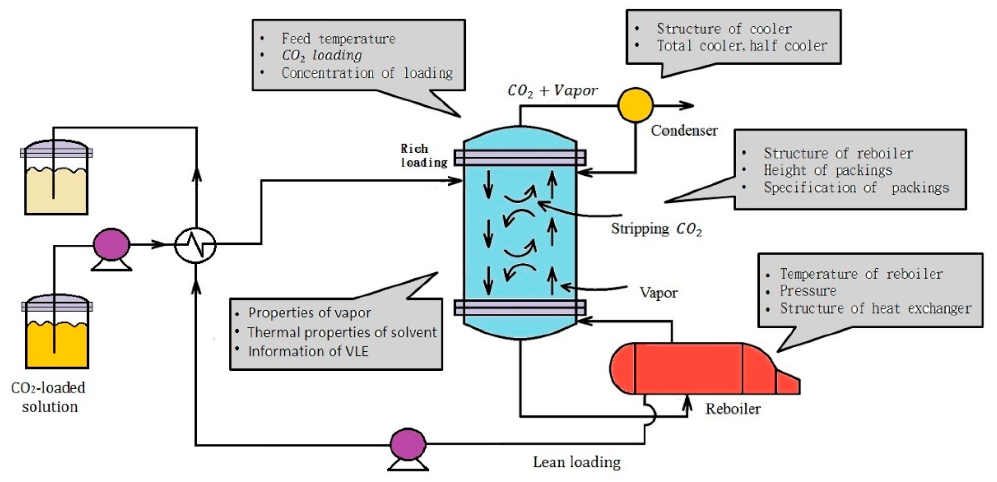
1. Introduction
2. Experimental Features
2.1. Experimental Design
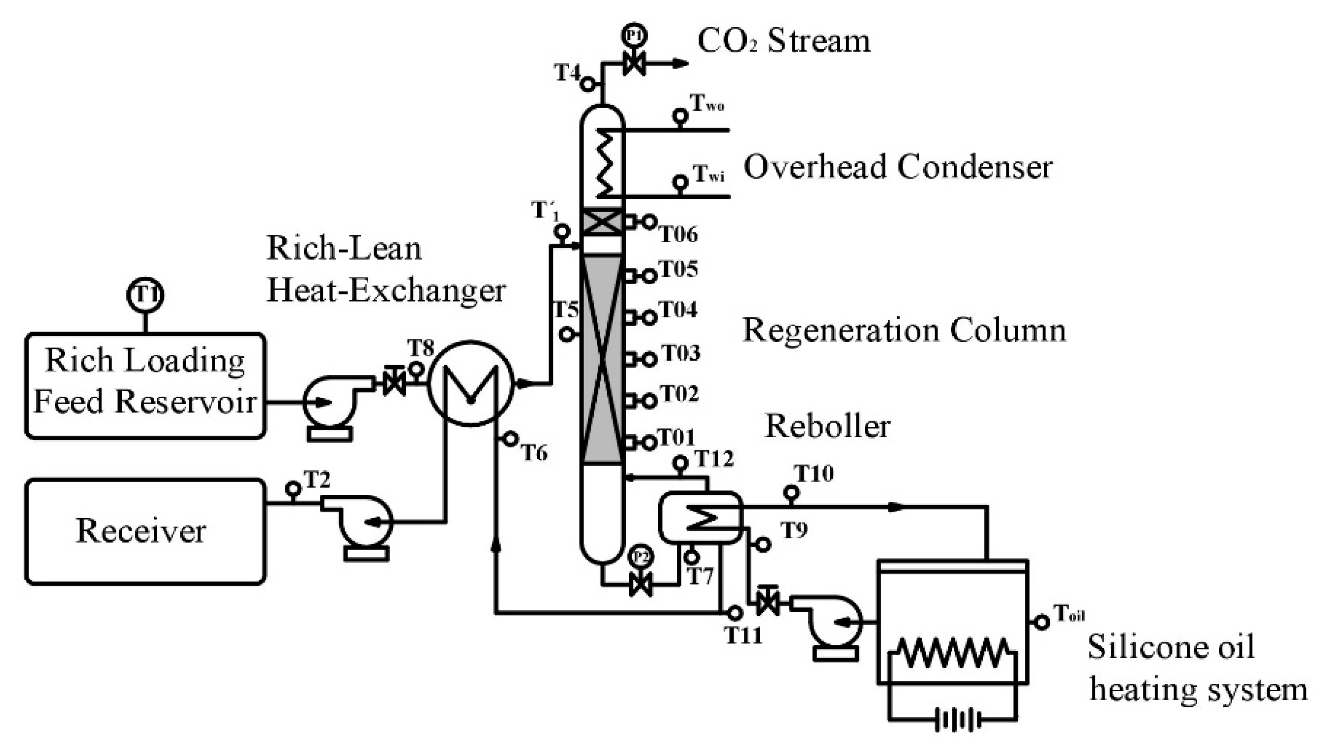
2.2. Experimental Device and Operating Procedure
| T1: | Inlet Temperature of Rich Loading | T7: | Reboiler Temperature | T12: | Steam Temperature |
| T2: | Temperature at outlet of heat exchanger | T8: | Inlet temperature of rich loading | Twi: | Inlet temperature of cooling water |
| T4: | Out temperature at the top of cooler | T9: | Oil temperature at the inlet of reboiler (Tin) | Two: | Outlet temperature of cooling water |
| T5: | Temperature of bed | T10: | Oil temperature at the outlet of reboiler (Tout) | P1: | Pressure valve at the top of tower |
| T6: | Liquid temperature at the inlet of heat exchanger | T11: | Outlet temperature the reboiler | P2: | Pressure valve at the bottom of tower |
2.3. Determination of Experimental Data
2.3.1. Stripping Efficiency
2.3.2. Stripping Rate of CO2
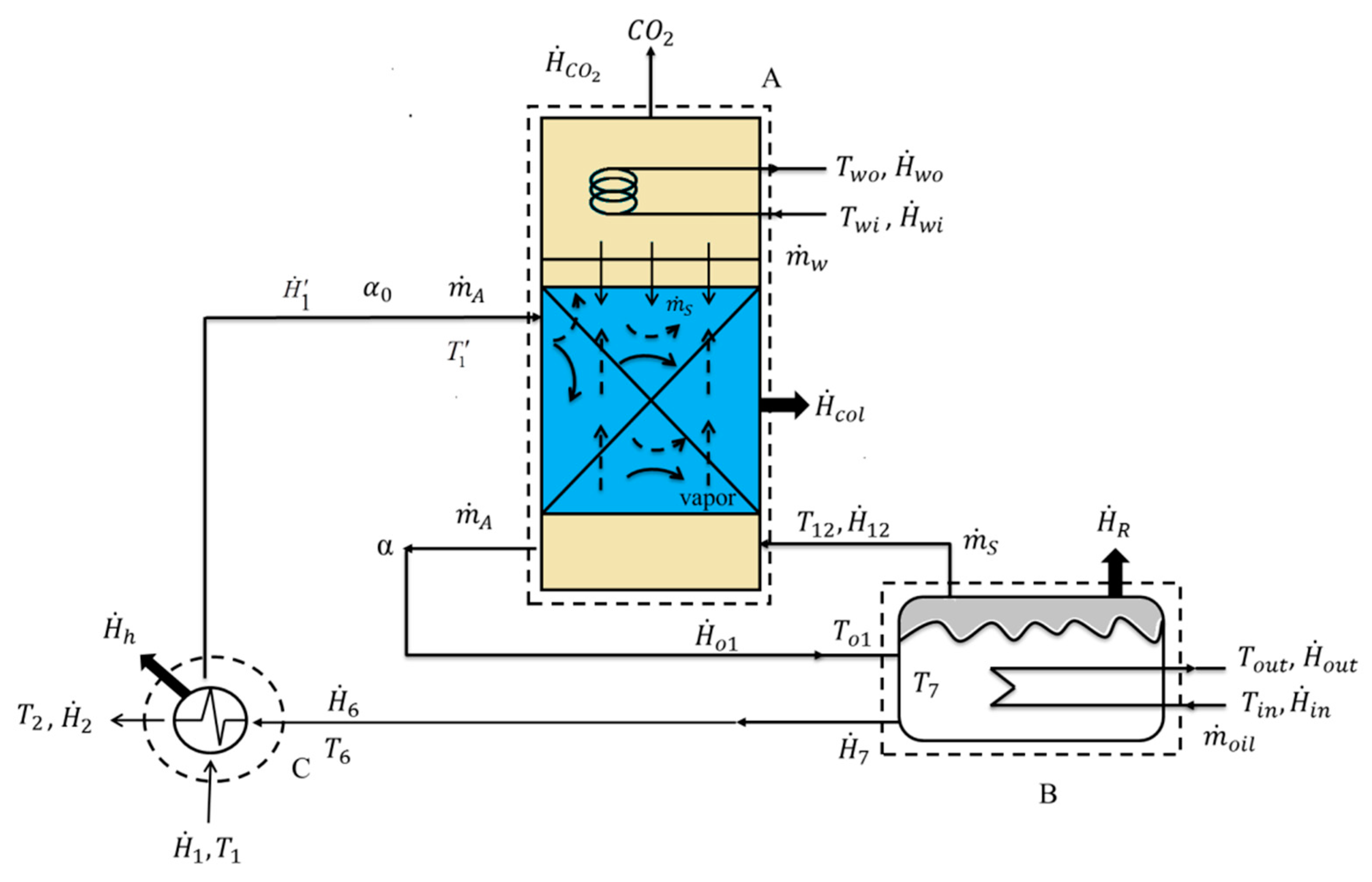
2.3.3. Enthalpy Balance for Heat of Regeneration
2.3.4. Steam Flow Rate
3. Results and Discussion
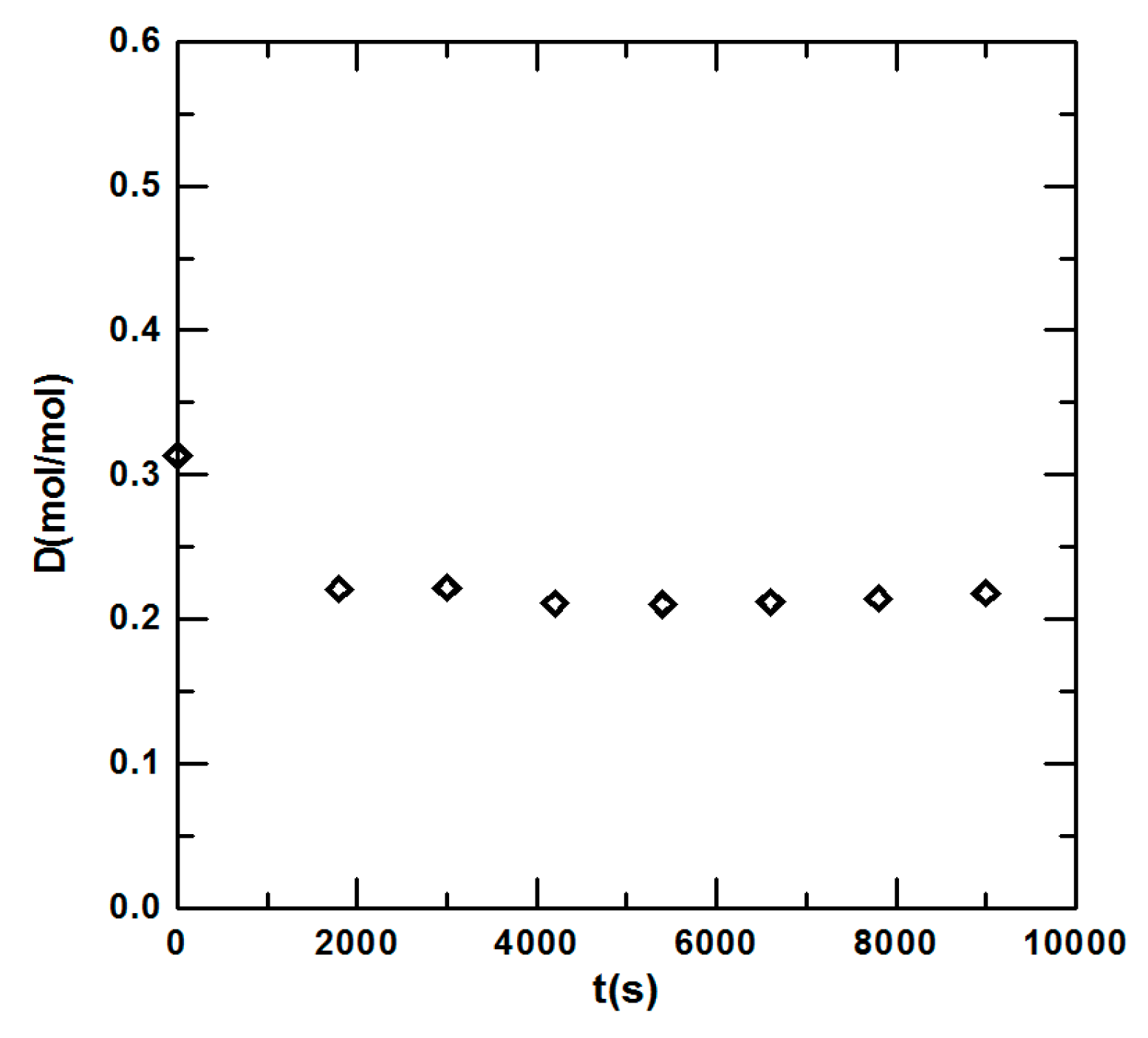
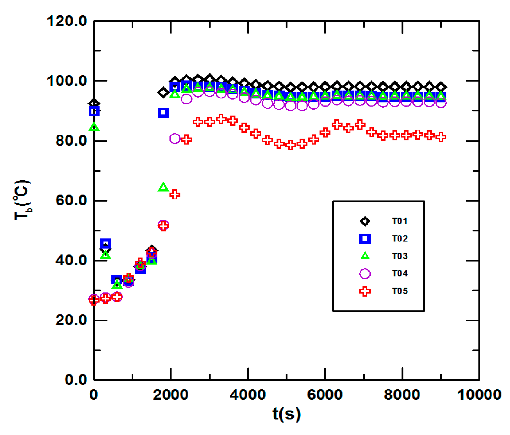
3.1. Steady State Operation
3.2. Taguchi Analysis
3.2.1. S/N Ratio for E
3.2.2. Confirmation of the Optimum Conditions
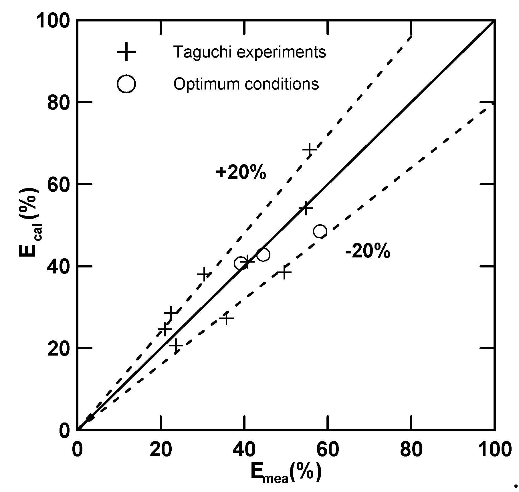
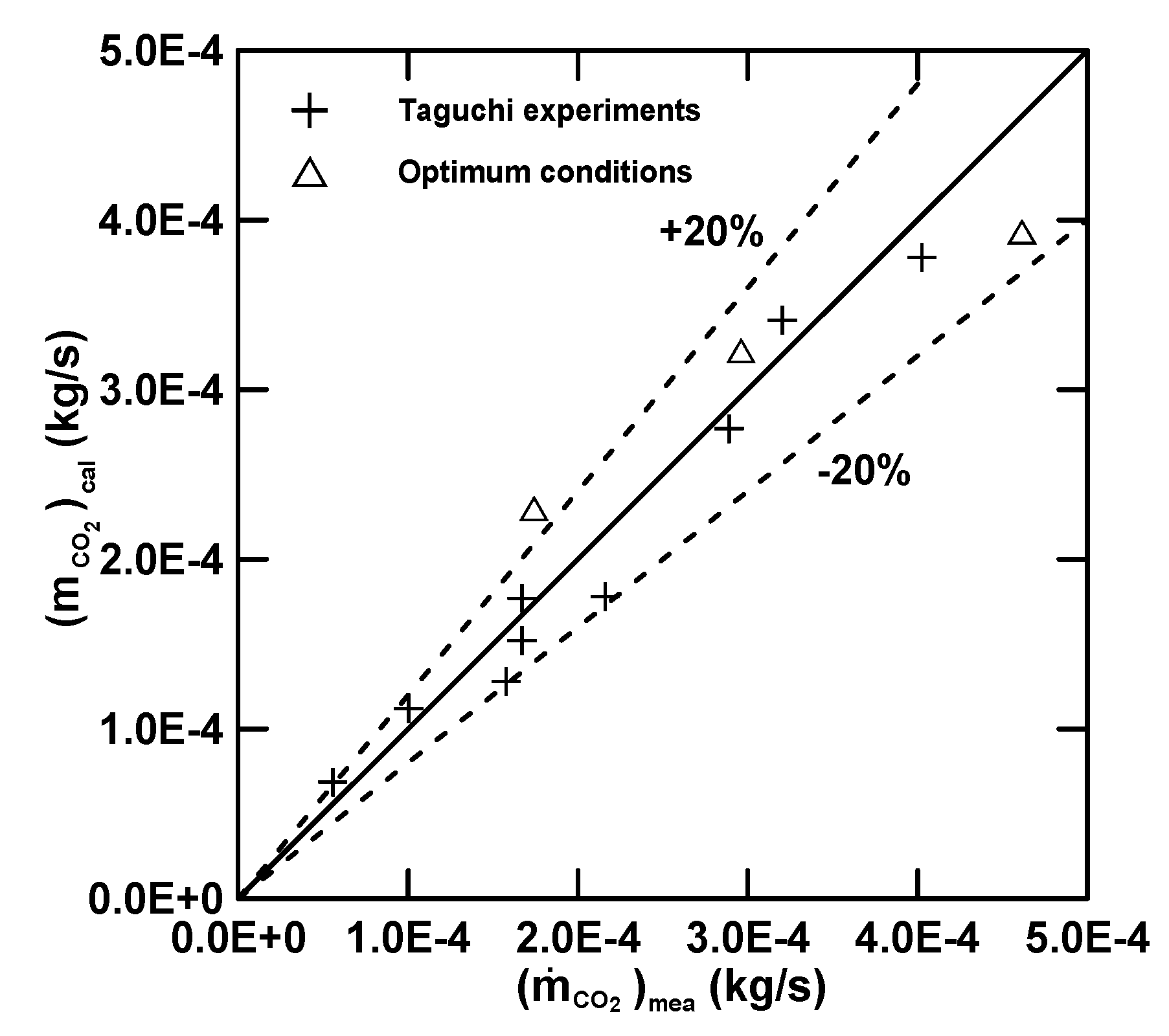
3.3. Empirical Equations
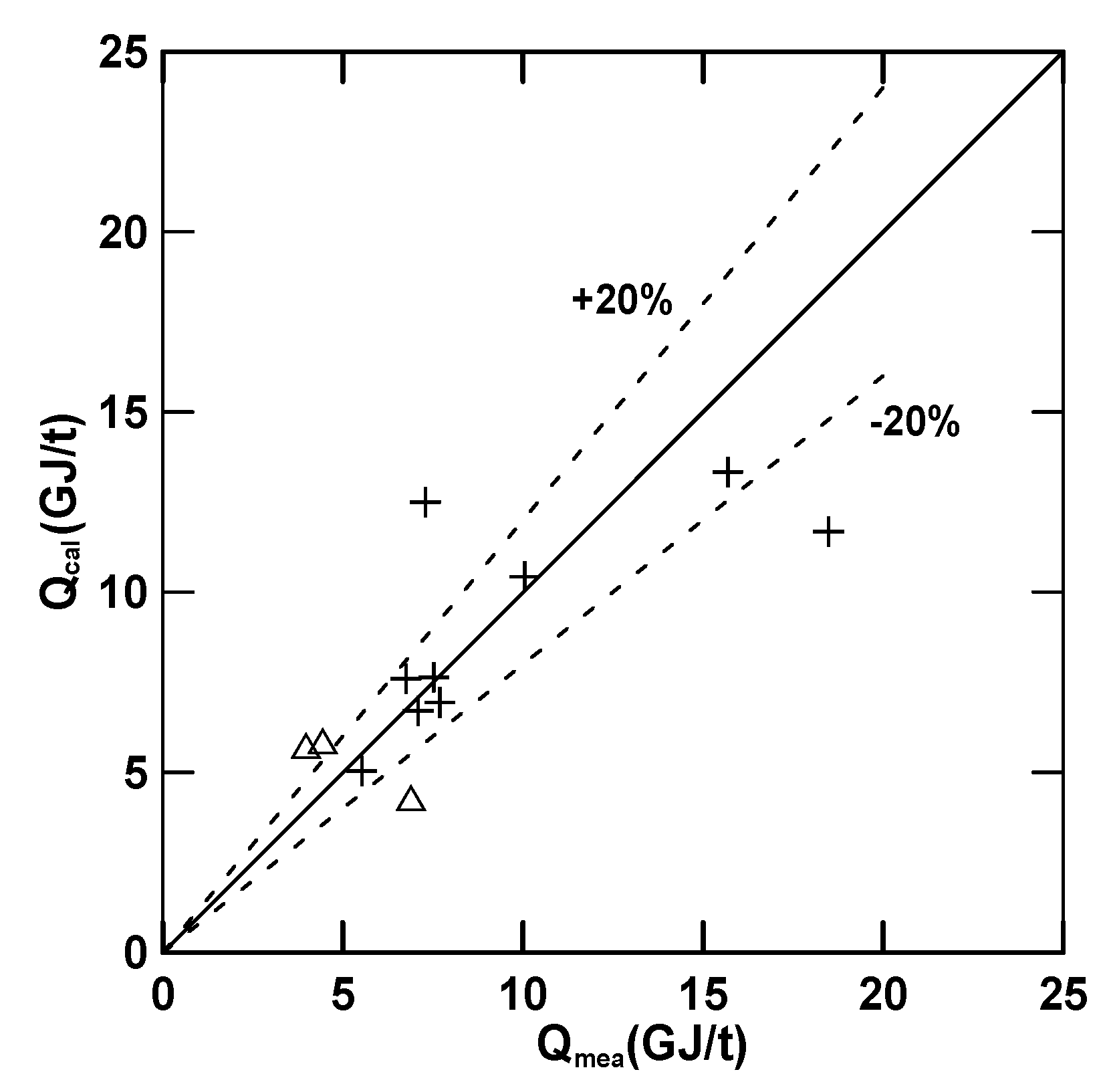
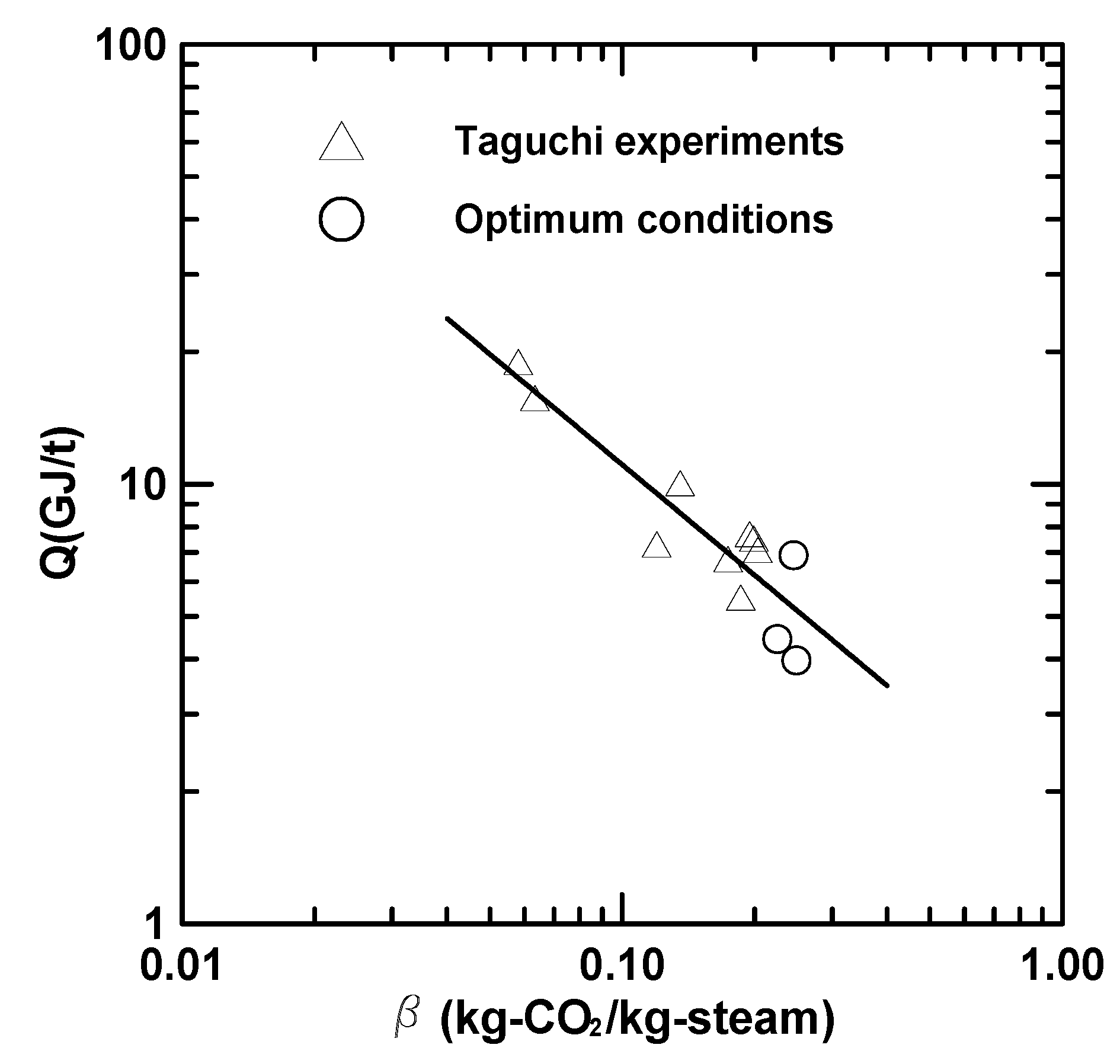
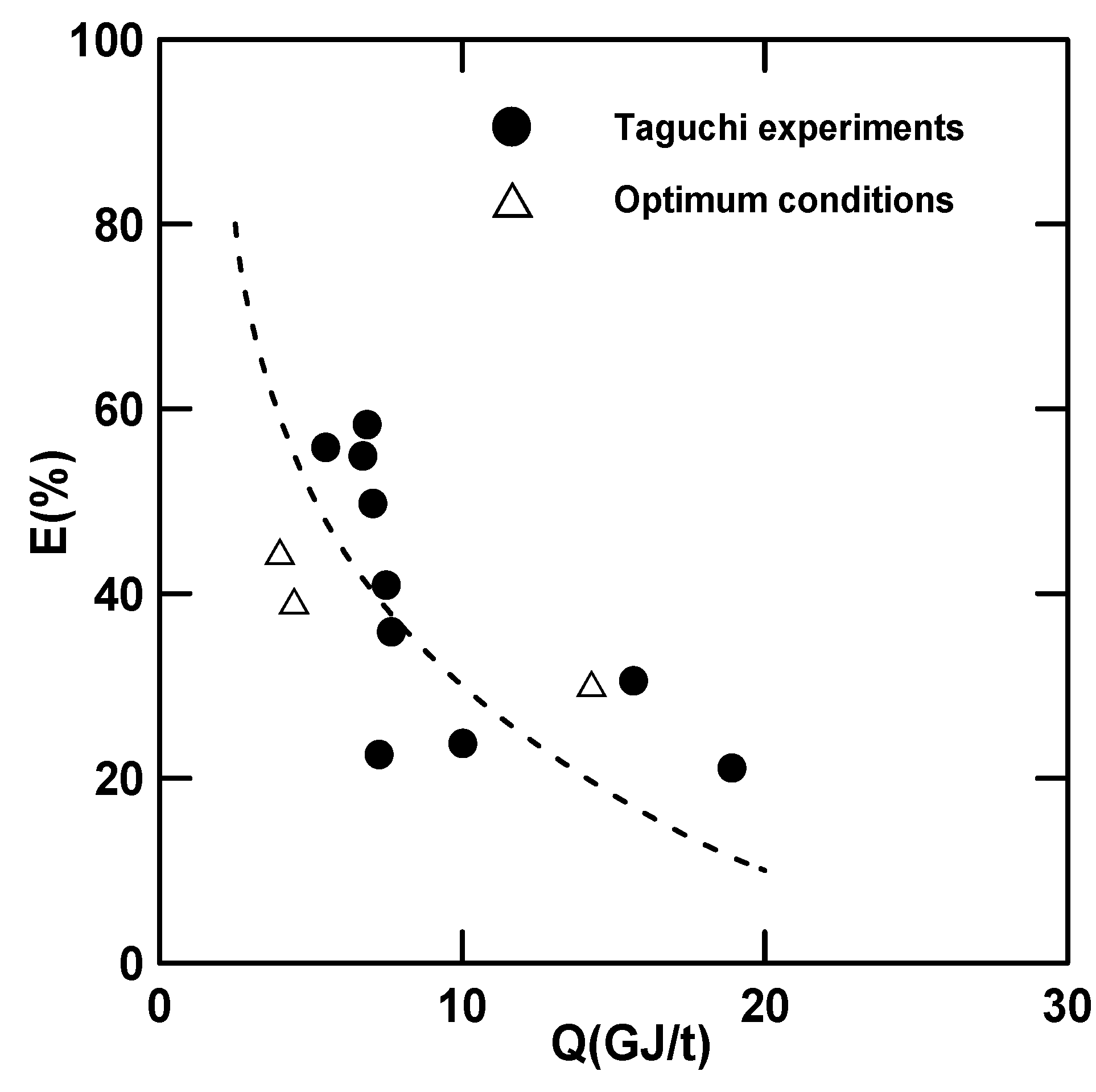
3.4. Heat of Regeneration and Stripping Factor
3.5. Policy in Operation
4. Conclusions
Author Contributions
Funding
Acknowledgments
Conflicts of Interest
Abbreviation
| AMP | 2-amino-2-methyl-1-propanol |
| AMPD | 2-amino-2-methyl-propane-1,3-diol |
| DETA | Diethylenetriamine |
| MEA | Monoethanolamine |
| PZ | Piperazine |
| PZEA | (Piperazinyl-1)-2-ethylamine |
| SG | Sodium glycinate |
| S/N | Signal/Noise |
| TETA | Triethylenetetramine |
Nomenclature
| C | kmol/m3 | concentration |
| CA | kmol/m3 | concentration of amine |
| CPw | kJ/kg·K | hat capacity of water |
| CPA | kJ/kg·K | hat capacity of amine |
| Cp,oil | kJ/kg·K | hat capacity of oil |
| E | % | stripping efficiency |
| kJ/s | reboiler heat loss | |
| kJ/s | column heat loss | |
| kJ/s | heat removed by cooler | |
| Hh | kJ/s | heat exchanger heat loss |
| Hvap | kJ/kg | heat of evaporation |
| kJ/s | total heat loss | |
| kJ/s | heat flow rate in reboiler | |
| kJ/s | enthalpy at inlet | |
| kJ/s | enthalpy at outlet | |
| Habs | kJ/kg | heat of absorption |
| kg/s | stripping rate | |
| kg/s | oil flow rate | |
| kg/s | steam generation rate | |
| kg/s | cooling water flow rate | |
| n | - | number of data points |
| kmol/s | amine flow rate | |
| Q | W | total heat flow |
| QA | m3/s | liquid volumetric flow rate |
| Qabs | kW | heat flow of absorption |
| Qsen | kW | sensitive heat flow |
| Qvap | W | heat flow of evaporation |
| Tin | K | temperature at inlet of reboiler |
| Tout | K | temperature at outlet of reboiler |
| To1 | K | temperature at the bottom of column |
| TR | K | reboiler temperature |
| Ts | K | steam temperature |
| Twi | K | inlet temperatureof the cooler |
| Two | K | outlet temperatureof the cooler |
| T1 | K | temperature at inlet of storage tank |
| tR | °C | reboiler temperature |
| zi | - | value of ith data |
| Greek Letters | ||
| α | kmol-CO2/kmol-amine | rich loading |
| α0 | kmol-CO2/kmol-amine | lean loading |
| β | kg-CO2/kg-steam | stripping factor |
References
- Li, T.; Keener, T.C. A review: Desorption of CO2 From Rich Solutions in Chemical Absorption Processes. Int. J. Greenh. Gas Control 2016, 51, 290–304. [Google Scholar] [CrossRef]
- Aronu, U.E.; Svendsen, H.F.; Hoff, K.A.; Juliussen, O. Solvent Selection for Carbon Dioxide Absorption. Energy Procedia 2009, 1, 1051–1057. [Google Scholar] [CrossRef]
- Adeosun, A.; Goetheer, N.E.H.; Abu-Zahra, M.R.M. Absorption of CO2 by Amine Blends Solution: An Experimental Evaluation. Int. J. Eng. Sci. 2013, 3, 12–23. [Google Scholar]
- Chen, P.C.; Lin, S.Z. Optimization in the Absorption and Desorption of CO2 Using Sodium Glycinate Solution. Appl. Sci. 2018, 8, 2041. [Google Scholar] [CrossRef]
- Chen, P.C.; Luo, Y.X.; Cai, P.W. Capture of Carbon Dioxide Using Monoethanolamine in a Bubble-Column Scrubber. Chem. Eng. Technol. 2015, 38, 274–282. [Google Scholar] [CrossRef]
- Choi, W.J.; Seo, J.B.; Seo, S.-Y.; Jung, J.H.; Oh, K.J. Removal Characteristics of CO2 Using Aqueous MEA/AMP Solutions in the Absorption and Regeneration Process. J. Environ. Sci. 2009, 21, 907–913. [Google Scholar] [CrossRef]
- Dash, S.K.; Sammanta, N.; Bandyopadhyay, S.S. Simulation and Parametric Study of Post Combustion CO2 Capture Process Using (AMP+PZ) Blended Solvent. Int. J. Greenh. Gas Control 2014, 21, 130–139. [Google Scholar] [CrossRef]
- Leung, D.Y.C.; Caramanna, G.; Maroto-Valer, M.M. An Overview of Current Status of Carbon Dioxide Capture and Storage Technologies. Renew. Sustain. Energy Rev. 2014, 39, 426–443. [Google Scholar] [CrossRef]
- Ho, M.T.; Allinson, G.W.; Wiley, D.E. Comparison of MEA Capture Cost for Low CO2 Emissions Sources in Australlia. Int. J. Greenh. Gas Control 2011, 5, 49–60. [Google Scholar] [CrossRef]
- Aroonwilas, A.; Veawab, A. Integration of CO2 Capture Unit Using Blended MEA-AMP Solution into Coal-Fired Power Plants. Energy Procedia 2009, 1, 4315–4321. [Google Scholar] [CrossRef]
- Kim, J.H.; Lee, J.H.; Lee, I.Y.; Jang, K.R.; Shim, J.G. Performance Evaluation of Newly Developed Absorbents for CO2 Capture. Energy Procedia 2011, 4, 81–84. [Google Scholar] [CrossRef]
- Han, K.; Ahn, C.K.; Lee, M.S. Performance of an Ammonia-Based CO2 Capture Pilot Facility in Iron and Steel Industry. Int. J. Greenh. Gas Control 2014, 27, 239–246. [Google Scholar] [CrossRef]
- Zhang, X.; Fu, K.; Liang, Z.; Yang, Z.; Rongwong, W.; Na, Y. Experimental Studies of Regeneration Heat Duty for CO2 Desorption from Aqueous DETA Solution in a Randomly Packed Column. Energy Procedia 2014, 63, 1497–1503. [Google Scholar] [CrossRef]
- Kwak, N.S.; Lee, J.H.; Lee, I.Y.; Jang, K.R.; Shim, J.G. A Study of New Absorbent for Post-Combustion CO2 Capture Test Bed. J. TIChE 2014, 45, 2459–2556. [Google Scholar] [CrossRef]
- Xiao, J.; Li, C.C.; Li, M.H. Kinetics of Absorption of Carbon Dioxide into Aqueous Solutions of 2-amino-2-methyl-1-propanol+Monoethanolamin. Chem. Eng. Sci. 2000, 55, 161–175. [Google Scholar] [CrossRef]
- Kumar, P.S.; Hogendoorn, J.A.; Versteeg, G.F.; Feron, P.H.M. Kinetics of the Reaction of CO2 With Aqueous Potassium Salt of Taurine and Glycine. Aiche J. 2003, 49, 203–213. [Google Scholar] [CrossRef]
- Singh, P.; Versteeg, G.F. Structure and Activity Relationships for CO2 Regeneration from Aqueous Amine-Based Absorbents. Process Saf. Environ. Prot. 2008, 86, 347–359. [Google Scholar] [CrossRef]
- Idem, R.; Wilson, M.; Tontiwachwuthikul, P.; Chakma, A.; Veawab, A.; Aroonwilas, A.; Gelowitz, D. Pilot Plant Studies of the CO2 Capture Performance of Aqueous MEA and Mixed MEA/MDEA Solvents at the University of Regina CO2 Capture Technology Development Plant and Boundary Dam CO2 Capture Demonstration Plant. Ind. Eng. Chem. Res. 2006, 45, 2414–2420. [Google Scholar] [CrossRef]
- Weiland, R.H.; Hatcher, N.A. Post-Combustion CO2 Capture with Amino-Acid Salts. In Proceedings of the GPA Europe Meeting, Lisbon, Portugal, 22–24 September 2010. [Google Scholar]
- Lin, P.H.; Shan, D.; Wong, H. Carbon Dioxide Capture and Regeneration with Amine/Alcohol/Water. Int. J. Greenh. Gas Control 2014, 26, 69–75. [Google Scholar] [CrossRef]
- Oexmann, J.; Kather, A. Minimising the Regeneration Heat Duty of Post-Combustion CO2 Capture by Wet Chemical Absorption: The Misguided Focus on Low Heat of Absorption Solvents. Int. J. Greenh. Gas Control 2010, 4, 36–43. [Google Scholar] [CrossRef]
- Veawab, V.; Aroonwilas, A. Energy Requirement for Solvent Regeneration in CO2 Capture Plants. In Proceedings of the 9th International CO2 Capture Network, Copenhagen, Denmark, 16 June 2006. [Google Scholar]
- Rochelle, G.T. Innovative Stripper Configurations to Reduce the Energy Cost of CO2 Capture. In Proceedings of the Second Annual Carbon Sequestration Conference, Alexandria, VA, USA, 5–8 May 2003. [Google Scholar]
- Esmaeili, H.; Roozbehani, B. Pilot-Scale Experiments for Post-Combustion CO2 Capture from Gas Fired Power Plants with a Novel Solvent. Int. J. Greenh. Gas Control 2014, 30, 212–215. [Google Scholar] [CrossRef]
- Yu, C.H.; Huang, C.H.; Tan, C.S. A Review of CO2 Capture by Absorption and Adsorption. Aerosol Air Qual. Res. 2012, 12, 745–769. [Google Scholar] [CrossRef]
- Rabensteiner, M.; Kinger, G.; Koller, M.; Gronald, G.; Unterberger, S.; Hochenauer, C. Investigation of the Suitability of Aqueous Sodium Glycinate as a Solvent for Post Combustion Carbon Dioxide Capture on the Basis of Pilot Studies and Screening Methods. Int. J. Greenh. Gas Control 2014, 29, 1–3. [Google Scholar] [CrossRef]
- Ali Khan, A.; Halder, G.N.; Saha, A.K. Carbon Dioxide Capture Characteristics from Flue Gas Using Aqueous 2-amino-2-methyl-1-propanal (AMP) and Monoethanolamine (MEA) Solutions in Packed Bed Absorption and Regeneration Columns. Int. J. Greenh. Gas Control 2015, 32, 15–23. [Google Scholar] [CrossRef]
- Badea, A.A.; Dinca, C.F. CO2 Capture from Post-Combustion Gas by Employing MEA Absorption Process—Experimental Investigation for Pilot Studies. U.P.B. Sci. Bull. Ser. D 2012, 74, 21–32. [Google Scholar]
- Van Wagener, D.H.; Rochelle, G.T. Stripper Configuration for CO2 Cpature by Aqueous Monoethhanolamine and Piperazine. Energy Procedia 2011, 4, 1323–1330. [Google Scholar] [CrossRef]
- Yeh, J.T.; Resnik, K.P.; Rygle, K.; Pennline, H.W. Semi-Batch Absorption and Regeneration Studies for CO2 Capture by Aqueous Ammonia. Fuel Process. Technol. 2005, 86, 1533–1546. [Google Scholar] [CrossRef]
- Yang, J.; Yu, X.; Yan, J.; Tu, S.T. CO2 Capture Using Solution Mixed with Ionic Lliquid. Ind. Eng. Chem. Res 2014, 53, 2790–2799. [Google Scholar] [CrossRef]
- Song, H.J.; Lee, S.; Park, K.; Lee, J.; Chand Spah, D.; Park, J.W.; Filburn, T.P. Simplified Estimation of Regeneration Energy of 30 wt% Sodium Glycinate Solution for Carbon Dioxide Absorption. Ind. Eng. Chem. Res. 2008, 47, 9925–9930. [Google Scholar] [CrossRef]
- Geankoplis, C.J. Transport Processes and Unit Operations; Allyn and Bacon, Inc.: Boston, MA, USA, 1983; pp. 244–250. ISBN 0-205-07788-9. [Google Scholar]
- Smith, J.M.; van Ness, H.C.; Abbott, M.M. Introduction to Chemical Engineering Thermodynamics; McGraw Hill: New York, NY, USA, 2006; pp. 116–125. ISBN 007-008304-5. [Google Scholar]
- Levenspiel, O. Chemical Reaction Engineering; Jon Wiley & Sons, Inc.: Hoboken, NJ, USA, 1999; pp. 28–29. ISBN 0-471-25424-X. [Google Scholar]


| Solvents | Conditions | Heat of Regeneration (GJ/t-CO2) | References |
|---|---|---|---|
| SG | Loading = 0.11–0.52 T = 100–120 °C 3–6 M SG | 3.68–10.75 | [4] |
| AMP + PZ | Loading = 0.46 L/G = 2.9 18 wt.% AMP + 17.5 wt.% PZ | 3.4–4.4 | [7] |
| DETA | Loading = 1.2–1.4 Solvent flow rate = 3–12 m3/m2-h 2–3 M DETA | 2.61–4.96 | [13] |
| ACOR100 (MEA + TETA +AMPD + PZEA) | Solvent flow rate = 0.4–0.8 L/min Partial pressure of CO2 = 54 mbar | 2.7–3.9 | [24] |
| KoSol-4 | Loading = 0.8 L/G = 1.4–3.1 kg/Sm3 P = 0.35–0.8 kg/cm2 | 3.0–4.1 | [14] |
| SG | Loading = 0.13–0.50 15–40 wt.% L/G = 2–10 L/m3 | 5.3–8.5 | [26] |
| AMP | Loading = 0.55 30 wt.% AMP | 2.1 | [27] |
| MEA | Loading = 0.25–0.49 30 wt.% MEA | 3.3–6.4 | [28] |
| PZ | Loading 0.4 T = 120–150 °C | 2.93–3.43 | [29] |
| Ammonia | Loading = 0.0525–0.01236 7–14% Ammonia | 11.25 | [30] |
| MEA MEA + ionic liquid + water | 30 wt.% MEA 30 wt.% + 40 wt.% + 30 wt.% T = 103 °C Simulation | 8.19 5.14 | [31] |
| SG MEA | 30 wt.% T = 40–120 °C Thermodynamic calculation | 5.7 4.7 | [32] |
| MEA + AMP | MEA:AMP = 2:1/1:1/1:2 T = 103–110 °C | 2.5–5.0 | [10] |
| Factor | 1 | 2 | 3 |
|---|---|---|---|
| CO2-loading (A) mol-CO2/mol-amine | 0.3 | 0.4 | 0.5 |
| Reboiler temperature (B)/°C | 100 | 110 | 120 |
| Feed rate (C)/m3/s | 3(10−4) | 6(10−4) | 9(10−4) |
| Concentration of solvent (D)/kmol/m3 | 4 | 5 | 6 |
| No. | A (kmol-CO2/kmol-amine) | B (°C) | C (m3/s) | D (kmol/m3) |
|---|---|---|---|---|
| 1 | 1 | 1 | 1 | 1 |
| 2 | 1 | 2 | 2 | 2 |
| 3 | 1 | 3 | 3 | 3 |
| 4 | 2 | 1 | 2 | 3 |
| 5 | 2 | 2 | 3 | 1 |
| 6 | 2 | 3 | 1 | 2 |
| 7 | 3 | 1 | 3 | 2 |
| 8 | 3 | 2 | 1 | 3 |
| 9 | 3 | 3 | 2 | 1 |
| No. | tR (°C) | CA (kmol/m3) | QA (104) (m3/s) | Q (GJ/t) | E (%) | |||||
|---|---|---|---|---|---|---|---|---|---|---|
| 1 | 0.31 | 0.22 | 100 | 4 | 3 | 15.69 | 5.57 | 8.82 | 0.063 | 30.43 |
| 2 | 0.31 | 0.24 | 110 | 5 | 6 | 7.29 | 10.04 | 8.38 | 0.120 | 22.45 |
| 3 | 0.30 | 0.22 | 120 | 6 | 9 | 18.94 | 16.71 | 30.63 | 0.058 | 20.98 |
| 4 | 0.41 | 0.30 | 100 | 6 | 6 | 10.05 | 16.71 | 12.34 | 0.144 | 23.64 |
| 5 | 0.41 | 0.25 | 110 | 4 | 9 | 7.52 | 28.91 | 14.52 | 0.199 | 40.79 |
| 6 | 0.39 | 0.13 | 120 | 5 | 3 | 6.75 | 15.77 | 9.06 | 0.174 | 54.78 |
| 7 | 0.51 | 0.34 | 100 | 5 | 9 | 7.69 | 40.26 | 20.67 | 0.195 | 35.73 |
| 8 | 0.50 | 0.25 | 110 | 6 | 3 | 7.08 | 21.59 | 10.62 | 0.203 | 49.63 |
| 9 | 0.49 | 0.18 | 120 | 4 | 6 | 5.52 | 32.04 | 17.21 | 0.186 | 55.70 |
| 10 | 0.55 | 0.21 | 120 | 4 | 3 | 6.89 | 17.41 | 7.10 | 0.245 | 58.18 |
| 11 | 0.47 | 0.26 | 120 | 5 | 9 | 3.97 | 46.15 | 19.24 | 0.236 | 44.54 |
| 12 | 0.52 | 0.31 | 110 | 5 | 6 | 4.44 | 29.61 | 13.14 | 0.225 | 39.20 |
| Level | A | B | C | D |
|---|---|---|---|---|
| 1 | 27.71 | 29.40 | 32.78 | 32.26 |
| 2 | 31.49 | 31.05 | 29.80 | 30.95 |
| 3 | 33.30 | 32.04 | 29.90 | 29.27 |
| Delta | 5.59 | 2.64 | 2.98 | 2.99 |
| Rank | 1 | 4 | 3 | 2 |
| S/N | Optimum Condition | Parameter Importance |
|---|---|---|
| E (Equation (2)) | A3B3C1D1 | A > D > C > B |
| (Equation (2)) | A3B3C3D2 | A > C > B > D |
| Q (Equation (1)) | A3B2C2D2 | A > D > B > C |
| No | Optimum Condition | E (%) | Q | |
|---|---|---|---|---|
| No. 10 | A3B3C1D1 | (58.18) | 17.41 | 6.89 |
| No. 11 | A3B3C3D2 | 44.54 | (46.15) | 3.97 |
| No. 12 | A3B2C2D2 | 39.20 | 29.61 | (4.44) |
| Outcome Data | Root Mean Relative Error (%) | Activation Energy (kJ/mol) | Exponent for Each Equation | ||
|---|---|---|---|---|---|
| α0 | CA | QA | |||
| Equation (16) (E) | 4.97 (R2 = 0.72) | 30.78 | 0.68 | −1.39 | −0.33 |
| Equation (17) () | 7.00 (R2 = 0.92) | 12.82 | 2.03 | −0.23 | 0.68 |
| Equation (18) () | 5.71 (R2 = 0.71) | 24.81 | −0.097 | 0.19 | 0.78 |
| Equation (19) (Q) | 7.91 (R2 = 0.56) | −7.45 | −1.45 | 0.35 | −0.011 |
© 2019 by the authors. Licensee MDPI, Basel, Switzerland. This article is an open access article distributed under the terms and conditions of the Creative Commons Attribution (CC BY) license (http://creativecommons.org/licenses/by/4.0/).
Share and Cite
Chen, P.C.; Lai, Y.-L. Optimization in the Stripping Process of CO2 Gas Using Mixed Amines. Energies 2019, 12, 2202. https://doi.org/10.3390/en12112202
Chen PC, Lai Y-L. Optimization in the Stripping Process of CO2 Gas Using Mixed Amines. Energies. 2019; 12(11):2202. https://doi.org/10.3390/en12112202
Chicago/Turabian StyleChen, Pao Chi, and Yan-Lin Lai. 2019. "Optimization in the Stripping Process of CO2 Gas Using Mixed Amines" Energies 12, no. 11: 2202. https://doi.org/10.3390/en12112202
APA StyleChen, P. C., & Lai, Y.-L. (2019). Optimization in the Stripping Process of CO2 Gas Using Mixed Amines. Energies, 12(11), 2202. https://doi.org/10.3390/en12112202