Abstract
The new electric power generation scenario, characterized by growing variability due to the greater presence of renewable energy sources (RES), requires more restrictive dynamic requirements for conventional power generators. Among traditional power generators, gas turbines (GTs) can regulate the output electric power faster than any other type of plant; therefore, they are of considerable interest in this context. In particular, the dynamic performance of a GT, being a highly nonlinear and complex system, strongly depends on the applied control system. Proportional–integral–derivative (PID) controllers are the current standard for GT control. However, since such controllers have limitations for various reasons, a model predictive control (MPC) was designed in this study to enhance GT performance in terms of dynamic behavior and robustness to model uncertainties. A comparison with traditional PID-based controllers and alternative model-based control approaches (feedback linearization control) found in the literature demonstrated the effectiveness of the proposed approach.
1. Introduction
Alternative methods for electric power generation with respect to conventional fossil-fuel-based plants have attracted an increasing amount of interest over the last decades. Indeed, climate change on the one hand and constant depletion of fossil fuels on the other have encouraged the development of renewable energy sources (RES) in the energy sector [1,2,3]. RES, being stochastic and unplannable, make managing the electric system harder, especially in terms of stability.
In light of this, since conventional energy sources have to meet more stringent requirements, gas turbine (GT) units play a key role thanks to their characteristics of high flexibility and fast response [4]. In order to best exploit GT features, the employed control system is of paramount importance. Regarding heavy-duty GTs, there are two main control objectives: making the power generated follow its reference as fast as possible, and keeping the exhaust gas temperature (EGT) exiting the machine constant. Today, traditional proportional–integral–derivative (PID)-based controllers are used for controlling GTs; however, they cannot effectively achieve the control objectives for different reasons. As a matter of fact, these linear controllers are not able to handle the nonlinearities of the GT system and the coupling between the power and temperature channels.
Therefore, model-based control techniques have been increasingly explored in this field. The feedback linearization (FBL) approach [5] first appeared in [6], where the authors proved the effectiveness of the model-based technique with respect to traditional controllers. However, such work is affected by some major limitations. For instance, one can observe that such a controller needs measurements of all the state variables to solve the control problem. In most cases, EGT measurement is a difficult task due to the relevant time constant of a thermometer that can endure such a high-stress installation environment.
In order to deal with a system state measure that is not exactly known, a robust approach has to be carried out. In this context, the sliding mode (SM) control theory of [5] was used for a reduced-order GT model in [7], while a more accurate fifth-order SM controller was designed in [8], which performed well. Given the complexity of the system, further efforts have to be made to overcome some current difficulties by exploring other modern control theories.
Hence, the aim of this study was to develop a controller according to the model predictive control (MPC) technique in order to investigate the feasibility and the potential of this approach for heavy-duty GTs. In particular, the controller was developed following the theory presented in [9,10]. Some MPC approaches can be found in this line of research. For instance, an explicit MPC controller was designed for transient stability in a power system in [11]. An elementary predictive control was designed in [12] on the basis of a simplified single-input single-output (SISO) model developed in [13]. Two MPC-based strategies for a micro-GT-based combined cooling, heating, and power system are presented in [14], while an MPC strategy was applied to obtain micro-GT speed control in [15]. In [16], a multi-input multioutput (MIMO) nonlinear MPC control was developed. Other MPC applications can be found in the field of thrust engines for aircrafts, such as in [17,18]. However, very few MPC applications for heavy-duty GTs have been designed. For instance, [19] used a nonlinear MPC (NMPC) based on a simplified heavy-duty GT MIMO model for frequency and temperature control. In [20], the authors proposed an MPC approach for frequency control and emission reduction, while in [21], an MPC strategy was applied to a heavy-duty gas turbine but based on a linear approximate model of the plant. Except for the research mentioned above, most authors have focused their attention on the application of innovative control systems to microturbines, where the combustion chamber temperature (CCT) does not assume a critical behavior and, therefore, there are far fewer restrictive dynamic performance limitations.
The main contributions of this paper can be summarized as follows:
- Design of an MPC controller able to minimize the power response time to rapid reference variations compatibly with the dynamic limitations imposed by the CCT.
- Development of an MPC controller based on a reduced-order GT model that can handle model uncertainties.
Finally, the performance determined by the MPC are compared with the ones given by traditional PID controllers (which are currently employed in actual GTs) and the FBL control designed in [6].
2. Gas Turbine Modeling
This section illustrates the GT model and the approximations carried out in order to achieve the simplified model used to design the proposed MPC controller. For the sake of brevity, in the definition of the accurate GT model, only the main steps are reported; the interested reader can refer to [6] for more details.
2.1. Accurate Gas Turbine Model
The GT system can be conceptually split into three main macrocomponents: compressor, combustion chamber (CC), and turbine. A symbolic scheme is shown in Figure 1.
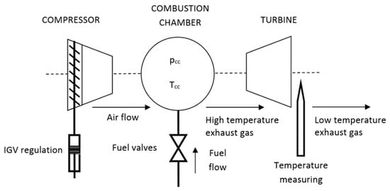
Figure 1.
Typical heavy-duty gas turbine (GT) schematic layout.
In particular, the following assumptions were made for the GT modeling:
- A single control volume is assumed regarding the CC and only two state variables describe the thermodynamic characteristics of the fluid inside it (i.e., the combustion chamber Pressure (CCP) and the CCT).
- The fluid inside the CC follows the ideal gas law.
- The fuel valve and the inlet guide vanes (IGV) can be modeled according to a linear first-order dynamic.
Considering the CC volume, the mass balance equation can be written as
where , , and are the air, fuel, and high-temperature exhaust gas mass flows, respectively, in kg/s; is the CC volume in m3; and is the CC air density in kg/m3. Thanks to the ideal gas law, can be expressed as
where is the CCP in Pa, is the CCT in K, and is the exhaust gas constant in J/kgK. Differentiating Equation (2) with respect to time, considering Equation (1), and applying the energy balance equation to the CC, one has
Applying the energy balance equation to the CC, one obtains
where is the specific heat at constant pressure in J/kgK, is the air temperature entering the CC in K, is the fuel lower heating value, is the enthalpy of the exhaust gas at the CC outlet in J/kgK, and is the internal energy of the control volume in J/kg. Thanks to the ideal gas assumption and recalling Equation (2), the following relation can be obtained:
where is the exhaust gas specific heat at constant pressure in J/kgK.
Finally, replacing Equation (1) in Equation (5) and considering Equation (4), one gets the dynamic equation of the CCT:
In addition, combining Equations (3) and (6), one obtains the dynamic equation of the CCP:
where and can be expressed as [6]
where and are the ambient temperature and pressure, respectively; , , and the rated values of the compressor air flow in kg/s, CCP in Pa, and temperature in K, respectively; and is the compressor efficiency.
With a good rate of accuracy, one can model the inlet systems according to the following dynamics:
where and are the desired air and fuel flows in kg/s, respectively, and and are the IGV and fuel valve time constant, respectively. In addition, as detailed later in the paper, the IGV is characterized by a maximum opening and closing speed which can be modeled only as a saturation-limiting .
The control objective for a heavy-duty GT installed in a combined cycle is to regulate the generated power (i.e., follow a power reference provided by the external primary controller) and to keep the EGT constant for the correct operation of the heat recovery steam generator (HRSG). The EGT can be computed considering an adiabatic transformation, leading to
where is the turbine adiabatic efficiency. In addition, if the control architecture needs to measure the EGT, the meter dynamics cannot be neglected, since the measurement of the EGT is quite challenging due the relevant mass flow and results in a very slow meter time constant .
The dynamics of the EGT measurement can be easily defined as follows:
On the other hand, the electric power can be obtained considering a simple balance between the mechanical power available at the turbine shaft and the power drained by the compressor. After a few passages, the electric power output as a function of the state variable becomes
where is the efficiency of the electric generator. As a general comment, the measurement of the electrical power is neglected since the time constant of power meters are much smaller than the thermal dynamics of the system.
Consequently, the accurate GT model results in a fifth-order nonlinear system, which can be written in the normal form as follows:
where the state vector x is
while the input vector is
and the system outputs are
In particular, one has
2.2. Heavy-Duty Gas Turbine Approximate Model
This section describes the approximations carried out on the model presented in the previous section to obtain a simpler model for the MPC controller design. These assumptions are generally valid for heavy-duty GTs and are introduced in order to simplify the design of the MPC controller and thus simplify implementation in industrial controllers. It is worth pointing out that these assumptions were only used to define the MPC control law, while the validation of the proposed control was done by providing the controller output to the accurate model of the GT. This also allowed us to prove the robustness of the proposed control approach.
The considered simplifications are:
- The actuator dynamics are neglected; hence, one obtains
- The dependence on the square root of the in Equation (8) is approximated with a simple inverse dependence, whereas the multiplicative coefficient becomes proportional to the rated CCT:where
- In Equation (6), the fuel lower heating value is much higher than the product ; that is,which leads to
- The MPC controller allows regulation of the desired quantities using only state measurements, which are necessary to predict the evolution of the desired output. For this reason, one could notice from Equation (11) that the evaluation of the EGT can only be done thanks to and . Since is not present in any other equation necessary to predict the dynamic evolution of the GT, this measurement is not necessary to perform the MPC control. This approximation is very important since it is well known that for a heavy-duty GT, EGT is a very limiting element due to the relevant meter units time constant [4].
Thanks to the approximations discussed above, the GT simplified model becomes
where
where , , , and are approximations of , , , and , respectively. In addition, one has
where the new constant parameters are defined as follows:
Thanks to the model described in Equation (27), the MPC controller can now be designed on a second-order dynamic system where the nonlinearities are much reduced with respect to system in Equation (14).
3. MPC Controller Design
3.1. Overview of the Model Predictive Control
Considering the following time-invariant affine discrete-time system,
where and denote states and inputs, respectively, at time , with as the sampling time.
The MPC controller acts to regulate system states to a reference value by solving a constrained quadratic programming (QP) problem:
where is the state vector error, refers to the prediction of the state at time calculated at time , and N is the prediction horizon. is the vector containing the optimal input vector , while and are symmetric and positive semidefinite weighting matrices. The , , , and matrices define the constraints for the controlled system. The control actions are generated by the MPC controller using this strategy: the quadratic optimization problem in Equation (40) is solved by the controller at each time step predicting the time evolution of the state variables and finally calculating the optimal input for the system within the control horizon. Then, only the first step is applied to the system while the rest of the solution U is just discarded. The control actions calculation process is then repeated at each time step .
If the considered model is not linear, a linearization procedure is required in order to obtain the system described in Equation (39). More details can be found in [10].
3.2. MPC Controller Design for a Heavy-Duty GT
The state dynamic Equation (27) of the heavy-duty GT can be rewritten as follows:
The mathematical model for prediction in the MPC controller of Equation (39) can be obtained performing the so-called “successive linearization” procedure used in [22]. This method consists of linearizing Equation (44) around a point at every sampling time step . Please note that such a point may not be a system equilibrium point. Performing the linearization procedure, system in Equation (44) can be reduced to the form
where the system matrices , , and at the considered sampling time step are defined as follows:
Then, due to the fact that the MPC control works in the discrete-time domain, Equation (45) needs to be discretized, and the zero-order hold discretization is performed as follows:
where the subscript k denotes system variables discretized at the sampling time .
In order to consider the physical bounds on air and fuel flow inlet systems, it is possible to insert into Equation (49) two new dynamic equations, where the inputs w are transformed into state variables and their derivatives and are considered as control variables for the system as follows:
Therefore, the resulting GT affine time-invariant discrete-time model for the prediction computed by the controller is
where
As stated before, dynamic Equation (52) is used to predict the evolution of the system in the MPC controller in order to satisfy the control goals of following a particular power reference and keeping the EGT constant. In order to satisfy control objectives, it is necessary to transform the system output references and into state-variables references in order to calculate the state error for the quadratic optimization problem described by Equation (40). This is possible by implementing a look-up table which is calculated by solving an algebraic system for each combination of and in steady-state conditions as follows:
The solution of system in Equation (58) is
and it can be implemented in the quadratic optimization problem of Equation (40). It is important to highlight that the values and coming from the solution of Equation (58) are not relevant in the optimization procedure because the corresponding state errors are not weighted in the control symmetric matrix Q (see Section 5).
Then, it is possible to define state and input limits with respect to the physical dynamic behavior of the heavy-duty GT as
which can be easily rewritten into the form described by the relations shown in Equations (42) and (43).
In summary, the heavy-duty GT MPC controller computes the optimal control action by minimizing the cost function in Equation (40), where the state error is defined as . The solution of the QP problem is carried out using Equation (52) as a prediction model and Equations (60)–(63) as input and state constraints. Then, and are applied to the nonlinear controlled system defined by Equation (14). For the sake of clarity, the control block diagram is reported in Figure 2.
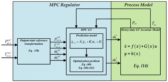
Figure 2.
Heavy-duty GT model predictive control (MPC) block scheme.
4. Simulation Results
The aim of this section is to evaluate the performance of the proposed MPC controller under realistic operational transients. As already pointed out in Section 2.2, the proposed controller was tested using as a testbed the accurate GT model defined in Section 2.1. This allowed determining the robustness of the proposed MPC controller in the presence of modeling uncertainties and against the assumption made for the controller design. In order to exhaustively assess the proposed MPC controller, its performances were evaluated in comparison with a traditional PID-based controller and an alternative model-based control technique, namely, the FBL technique, which has already been applied to control heavy-duty GTs [6]. As a matter of fact, the FBL procedure leads to an equivalent linear relationship between the controlled outputs and the fictitious inputs, as shown in Figure 3 [5].
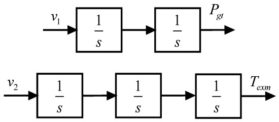
Figure 3.
Equivalent relation between fictitious inputs and the controlled quantities.
Considering this, the following equations can be written:
where and represent the poles of the two closed loop dynamics. By choosing , , the resulting control gains and can be easily calculated.
It is worth mentioning that the FBL controller proposed in [6] was designed on a fifth-order GT model and, thus, it has an intrinsic drawback related to the complexity of the control law definition that could make it impractical for industrial controller device implementation.
The parameters of the proposed MPC controller are reported in Table 1, while the parameters used for the FBL controller are reported in Table 2.

Table 1.
MPC controller parameters.
Table 2.
Feedback linearization (FBL) controller parameters [6].
As far as PID controllers are concerned, two different sets of parameters have been defined in Table 3, since heavy-duty GT operation is usually a trade-off between the time response of the power channel and the preservation of the machine lifetime by avoiding CCT spikes. Thus, the first set of PID parameters were proposed in order to achieve a quick power response leading to dangerous CCT dynamics (hereinafter referred to as ), while the second set of parameters were defined in order to preserve the CCT dynamics and thus provide a slower power response (hereinafter referred to as PID2).
Table 3.
Proportional–integral–derivative (PID) controller parameters.
The GT model parameters defined at °C and are reported in Table 4.
Table 4.
GT system model parameters.
The proposed controller was tested in two different operational conditions: a power reference step increase and a power reference step decrease.
4.1. Power Reference Step Increase
For this simulation test case, the machine was initially operated with a power production of 150 MW, and after 2 s, a step power increase to 250 MW was provided. The EGT reference was kept constant at 570 °C.
As one can observe from Figure 4, the MPC controller action provided the fastest power response (continuous red line) with respect to the FBL controller (dash dot green line), which provided a slightly lower performance, and both the PID controllers (dotted blue and magenta lines). Also, the EGT behavior was preferable in the MPC case, as shown in Figure 5, since it was the one characterized by the lower variation (less than 1 °C).
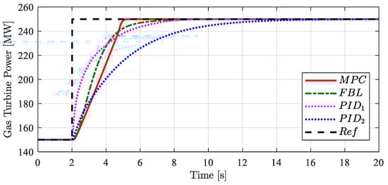
Figure 4.
Power production time profile.
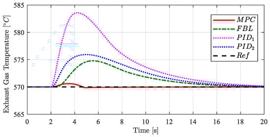
Figure 5.
Exhaust gas temperature (EGT) time profile.
Figure 6 reports the CCP and one can notice how none of the proposed control techniques provided critical time profiles. The same cannot be said for the CCT, shown in Figure 7, where one can observe the relevant peak provided by the controller and the slight peak provided by the FBL controller. On the contrary, the MPC controller provided a smoother profile characterized by no overshoot. The same result was obtained by the controller, which was designed to avoid such behavior; however, this resulted in a drastic reduction of the power performances, as shown in Figure 4. The MPC controller was able to accomplish both control objectives, achieving a fast power response and avoiding dangerous stresses in the CC at the same time.
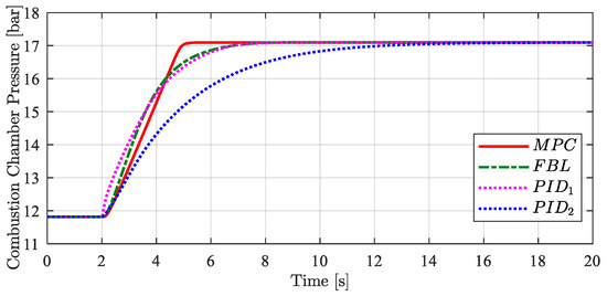
Figure 6.
Combustion chamber pressure (CCP) time profile.
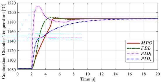
Figure 7.
Combustion chamber temperature (CCT) time profile.
Finally, for the sake of completeness, Figure 8 and Figure 9 show the air and fuel flow time profiles, respectively, in order to show the feasibility of the controllers request and the inclusion of actuators in the model used for simulating the GT process (neglected in the MPC controller design).
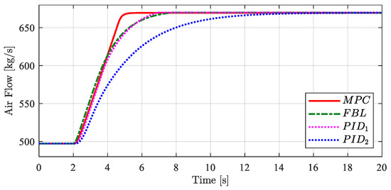
Figure 8.
Air flow time profile.
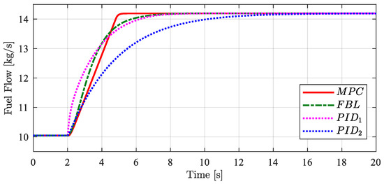
Figure 9.
Fuel flow time profile.
On balance, the MPC controller provided the best results in terms of response speed and CCT profile, even if it neglected some system dynamics considered instead by the FBL controller of [6].
4.2. Power Reference Step Decrease
For the power reference step decrease test case, the GT was initialized with a power production of 250 MW, and after 2 s, a step power decrease was provided which led to a final power production of 180 MW. As before, the EGT reference was kept constant at 570 °C.
This second scenario was less critical, since CCT dynamics are not dangerous for negative gradients. For this reason, the most important aspect for power load decrease is the fast time response of the electric power.
As one can see from Figure 10, the MPC controller provided the quickest power response, reaching the final reference value in almost 2 s. The EGT time profile again slightly changed, providing a good time response, as one can see from Figure 11.
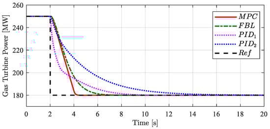
Figure 10.
Power production time profile.
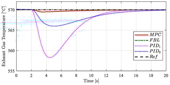
Figure 11.
EGT time profile.
The CCP and CCT dynamics, reported in Figure 12 and Figure 13, respectively, highlight the best performances of the MPC controller even if no particular requirements were provided for power reduction transients.
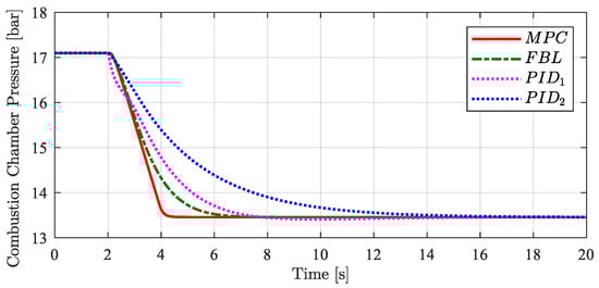
Figure 12.
CCP time profile.
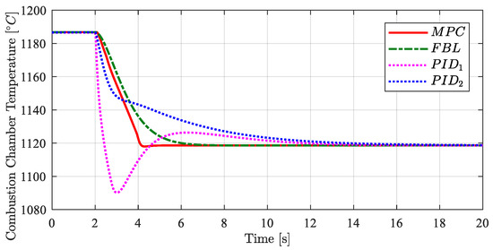
Figure 13.
CCT time profile.
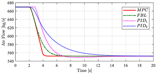
Figure 14.
Air flow time profile.
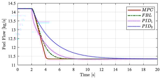
Figure 15.
Fuel flow time profile.
As a final comment, the reported results show improved performances of the MPC controller under all considered operation transients with respect to traditional PID-based controllers, while the comparison with the FBL control technique is similar, even if in many cases the MPC controller dynamics are faster and smoother. Nevertheless, the major simplicity of the MPC controller implementation would make its application far more appealing than FBL.
5. Conclusions
This paper proposed the design of an MPC for heavy-duty GTs based on a simplified second-order nonlinear model. The effectiveness of this controller was proved by applying it on a more complex GT model (i.e., a fifth-order model). The performances obtained thanks to the MPC were compared with those determined by state-of-the-art regulators (PID-based controllers) and a more sophisticated model-based control technique (based on the FBL control technique). Simulations highlighted that that the proposed MPC provided much higher performance with respect to the FBL controller, even if the FBL controller had been designed using a more complex model, namely, the fifth-order GT model. In addition, the PID controllers had lower performances and required finding a trade-off between different tuning assets (i.e., fast power response tuning and CCT peak avoidance tuning). In both cases, the electrical power and the CCT dynamic behaviors resulting from the MPC were significantly improved.
Author Contributions
A.R. designed the MPC controller and together with A.P. and D.L. performed the simulations and wrote the paper. A.B. and R.P. provided supervision to the research activity, provided critical analysis to the results achieved by comparative simulation and revised the manuscript.
Funding
This research received no external funding.
Conflicts of Interest
The authors declare no conflict of interest.
References
- Sims, R.E.; Schock, R.N.; Adegbululgbe, A.; Fenhann, J.V.; Konstantinaviciute, I.; Moomaw, W.; Nimir, H.B.; Schlamadinger, B.; Torres-Martinez, J.; Turner, C. Energy supply. In Proceedings of the Climate Change 2007: Mitigation. Contribution of Working Group III to the Fourth Assessment Report of the Intergovernmental Panel on Climate Change; Cambridge University Press: Cambridge, UK, 2007. [Google Scholar]
- Dresselhaus, M.; Thomas, I.J.N. Alternative energy technologies. Nature 2001, 414, 332–337. [Google Scholar] [CrossRef] [PubMed]
- Panwar, N.L.; Kaushik, S.C.; Kothari, S. Role of renewable energy sources in environmental protection: A. review. Renew. Sustain. Energy Rev. 2011, 15, 1513–1524. [Google Scholar] [CrossRef]
- Saravanamuttoo, H.I.; Rogers, G.F.C.; Cohen, H. Gas. Turbine Theory; Pearson Education: London, UK, 2001. [Google Scholar]
- Slotine, J.-J.E.; Li, W. Applied Nonlinear Control (No. 1); Prentice Hall: Englewood Cliffs, NJ, USA, 1991. [Google Scholar]
- Bonfiglio, A.; Cacciacarne, S.; Invernizzi, M.; Procopio, R.; Schiano, S.; Torre, I. Gas turbine generating units control via feedback linearization approach. Energy 2017, 121, 491–512. [Google Scholar] [CrossRef]
- Bonfiglio, A.; Invernizzi, M.; Lanzarotto, D.; Palmieri, A.; Procopio, R. Definition of a sliding mode controller accounting for a reduced order model of gas turbine set. In Proceedings of the 52nd International Universities Power Engineering Conference (UPEC), Heraklion, Greece, 28–31 August 2017; pp. 1–6. [Google Scholar]
- Bonfiglio, A.; Cacciacarne, S.; Invernizzi, M.; Lanzarotto, D.; Palmieri, A.; Procopio, R. A Sliding Mode Control Approach for Gas Turbine Power Generators. IEEE Trans. Energy Convers. 2018, 34, 921–932. [Google Scholar] [CrossRef]
- Camacho, E.F.; Alba, C.B. Model. Predictive Control; Springer Science & Business Media: Berlin, Germany, 2013. [Google Scholar]
- 1llgöwer, F.; Zheng, A. Nonlinear Model. Predictive Control; Birkhäuser: Basel, Switzerland, 2012. [Google Scholar]
- Bonfiglio, A.; Cantoni, F.; Oliveri, A.; Procopio, R.; Rosini, A.; Invernizzi, M.; Storace, M. An MPC-based Approach for Emergency Control ensuring Transient Stability in Power Grids with Steam Plants. IEEE Trans. Ind. Electron. 2018, 66, 5412–5422. [Google Scholar] [CrossRef]
- Jurado, F.; Acero, N.; Echarri, A. Enhancing the Electric System Stability using Predictive Control of Gas Turbines. In Proceedings of the 2017 Canadian Conference on Electrical and Computer Engineering, Ottawa, ON, Canada, 7–10 May 2006; pp. 438–441. [Google Scholar]
- Jurado, F. Modelling micro-turbines using Hammerstein models. Int. J. Energy Res. 2005, 29, 841–855. [Google Scholar] [CrossRef]
- Zhu, M.; Wu, X.; Li, Y.; Shen, J.; Zhang, J. Modeling and model predictive control of micro gas turbine-based combined cooling, heating and power system. In Proceedings of the 2016 Chinese Control and Decision Conference (CCDC), Yinchuan, China, 28–30 May 2016; pp. 65–70. [Google Scholar]
- Surendran, S.; Chandrawanshi, R.; Kulkarni, S.; Bhartiya, S.; Nataraj, P.S.V.; Sampath, S. Model predictive control of a laboratory gas turbine. In Proceedings of the 2016 Indian Control Conference (ICC), Hyderabad, India, 4–6 January 2016; pp. 79–84. [Google Scholar]
- Wiese, A.; Blom, M.; Manzie, C.; Brear, M.; Kitchener, A. Model reduction and MIMO model predictive control of gas turbine systems. Control. Eng. Pract. 2015, 45, 194–206. [Google Scholar] [CrossRef]
- Brunell, B.J.; Bitmead, R.R.; Connolly, A.J. Nonlinear model predictive control of an aircraft gas turbine engine. In Proceedings of the 41st IEEE Conference on Decision and Control, Las Vegas, NV, USA, 10–13 December 2002; Volume 4, pp. 4649–4651. [Google Scholar]
- Diwanji, V.; Godbole, A.; Waghode, N. Nonlinear Model Predictive Control for Thrust Tracking of a Gas Turbine. In Proceedings of the 2006 IEEE International Conference on Industrial Technology, Mumbai, India, 15–17 December 2006; pp. 3044–3048. [Google Scholar]
- Kim, J.S.; Powell, K.M.; Edgar, T.F. Nonlinear model predictive control for a heavy-duty gas turbine power plant. In Proceedings of the American Control Conference (ACC), Washington, DC, USA, 17–19 June 2013; pp. 2952–2957. [Google Scholar]
- Pires, T.S.; Cruz, M.E.; Colaço, M.J.; Alves, M.A. Application of nonlinear multivariable model predictive control to transient operation of a gas turbine and NOX emissions reduction. Energy 2018, 149, 341–353. [Google Scholar] [CrossRef]
- Ghorbani, H.; Ghaffari, A.; Rahnama, M. Constrained model predictive control implementation for a heavy-duty gas turbine power plant. WSEAS Trans. Syst. Control 2008, 3, 507–516. [Google Scholar]
- Oliveri, A.; Lodi, M.; Storace, M. High-speed explicit nonlinear model predictive control. In Proceedings of the 2017 European Conference on Circuit Theory and Design (ECCTD), Catania, Italy, 4–6 September 2017; pp. 1–4. [Google Scholar]
© 2019 by the authors. Licensee MDPI, Basel, Switzerland. This article is an open access article distributed under the terms and conditions of the Creative Commons Attribution (CC BY) license (http://creativecommons.org/licenses/by/4.0/).