A Multi-Objective Optimization Dispatch Method for Microgrid Energy Management Considering the Power Loss of Converters

Abstract

With the spreading and applying of microgrids, the economic and environment friendly microgrid operations are required eagerly. For the dispatch of practical microgrids, power loss from energy conversion devices should be considered to improve the efficiency. This paper presents a two-stage dispatch (TSD) model based on the day-ahead scheduling and the real-time scheduling to optimize dispatch of microgrids. The power loss cost of conversion devices is considered as one of the optimization objectives in order to reduce the total cost of microgrid operations and improve the utility efficiency of renewable energy. A hybrid particle swarm optimization and opposition-based learning gravitational search algorithm (PSO-OGSA) is proposed to solve the optimization problem considering various constraints. Some improvements of PSO-OGSA, such as the distribution optimization of initial populations, the improved inertial mass update rule, and the acceleration mechanism combining the memory and community of PSO, have been integrated into the proposed approach to obtain the best solution for the optimization dispatch problem. The simulation results for several benchmark test functions and an actual test microgrid are employed to show the effectiveness and validity of the proposed model and algorithm.

1. Introduction

The increasing seriousness of the energy crisis and environment preservation create new challenges for the energy industry. How to improve the utilization efficiency of energy while reducing power production costs and solving pollution problems? The emergence of microgrids has brought new effective technology to solve the problems facing the current energy industry. With the development of renewable energy (wind, solar, etc.) generation technology, the renewable energy source is increasingly used as a distributed generation (DG) unit in microgrids. However, the higher intermittent of renewables would lead to power fluctuation, that means coordinated operation of microgrids cannot be implemented. Energy management is the premise and basis of the coordinated operation for microgrids; economic optimization dispatch (EOD) is an attractive issue in terms of goals pursued (minimum-cost, maximum-profit and/or reliable operation, environment concern) and can face towards the operator and customer at the same time.

The economy and the environmental benefits of microgrid operation are the key to solving the EOD problem. So far, many researchers have developed solutions and strategies to handle the optimization dispatching under different objective and constraint conditions [1,2,3]. In general, the dispatch problem is seen as an optimization problem to minimize the operation costs. The authors in [2] proposed a novel battery operating cost model to maximize the efficient and the cycle life of the batteries, without considering additional objective functions of optimal scheduling for microgrid operation. While the optimization dispatch of microgrid to simplify the objectives into single-objective optimization dispatch (SOOD) problem may be acceptable in some situations, only considering the SOOD has lead to either neglecting certain benefits or changing constraint conditions, and different distributed generation units have different objectives or sets of objectives.

The multi-objective optimization dispatch (MOOD) approaches are developed in articles to obtain optimal scheduling plans for supplying the load under constraint conditions while taking minimum levels of cost, emission cost and other goals for microgrid operation [4,5,6,7,8]. In [9], an energy management model based on day-ahead scheduling is proposed to optimize two objectives, the total operation cost and the CO${}_2$ emission cost. In addition, the authors in [10,11] present an optimization dispatch approach for microgrid operation in order to reduce the operation cost and improve environmental friendliness. The MOOD approach lets us weigh among several competing objective functions and explicitly consider the effect of different objective functions within microgrid operation [12,13,14]. However, the power loss from a large amount of energy conversion devices installed in the microgrid system has been ignored when solving the MOOD problem. The major losses of each converter come from device conduction, switching and inductor [15]. According to the related literature, the maximum power loss of converters can reach up to 16% of conversion power, the minimum power loss is also equivalent to 2% conversion power [16,17]. Therefore, the power loss is considered as one of the optimization objectives to solve the MOOD problem in this paper, and the optimal solution of the MOOD problem is to improve the profit of the operator and utilize efficiency of distributed energy.

Many optimization methods have been proposed to solve the MOOD problem, which is a multi-objective, multi-constraint and non-linear optimization problem. According to some published articles, the optimization techniques are mainly classified into three groups, the traditional mathematical methods, the intelligent optimization methods and hybrid methods. The traditional mathematical methods, such as dynamic programming [18], stochastic dynamic programming [19], linear programming [20] and mixed-integer linear programming [21], are applied to solve optimization dispatch problems on different microgrids. These methods are used for large-scale optimization problems, and some methods are computationally fast. However, the traditional mathematical methods are not suitable for the optimization dispatch of a microgrid that is a non-linear, non-smooth and non-convex problem. Considering the features of the MOOD problem, many intelligent methods are used to handle the optimization dispatch of a microgrid. For instance, the genetic algorithm (GA) [22,23], particle swarm optimization (PSO) [24,25], the strength Pareto evolutionary algorithm (SPEA) [26] and so on have been increasingly proposed for solving the optimization dispatch problem because of their non-linear mapping, simplicity and powerful search capability. However, the above intelligent methods present the following shortcomings: many parameters are required to set before the optimization and most test cases are parameters sensitive, and a single intelligent optimization method is usually easy to fall into local optimum.

Hybrid method is a technology of integrating two or more different methods to solve the MOOD problem for a microgrid, and has become a hotspot in research now. Hybrid methods can utilize the advantages coming from the different methods, and usually obtains satisfied solutions for optimization dispatch problems in microgrids more easily. Recently, gravitational search algorithm (GSA) was proposed in [27]; it is a heuristic optimization algorithm based on Newton’s law of gravity and has high computational efficiency without sacrificing accuracy. The advantages and performances of GSA for optimization dispatch problems of microgrids have already been proven [28], and the convergence of GSA is better than the convergence of particle swarm optimization (PSO) and genetic algorithm (GA) [29]. Therefore, the aim of this work is to propose a two-stage dispatch (TSD) model combining the day-ahead scheduling and the real-time scheduling for optimization dispatches of microgrids. A hybrid particle swarm optimization and opposition-based learning gravitational search algorithm (PSO-OGSA) is proposed to solve this complicated constrained MOOD problem. The major contribution of this paper includes the following:

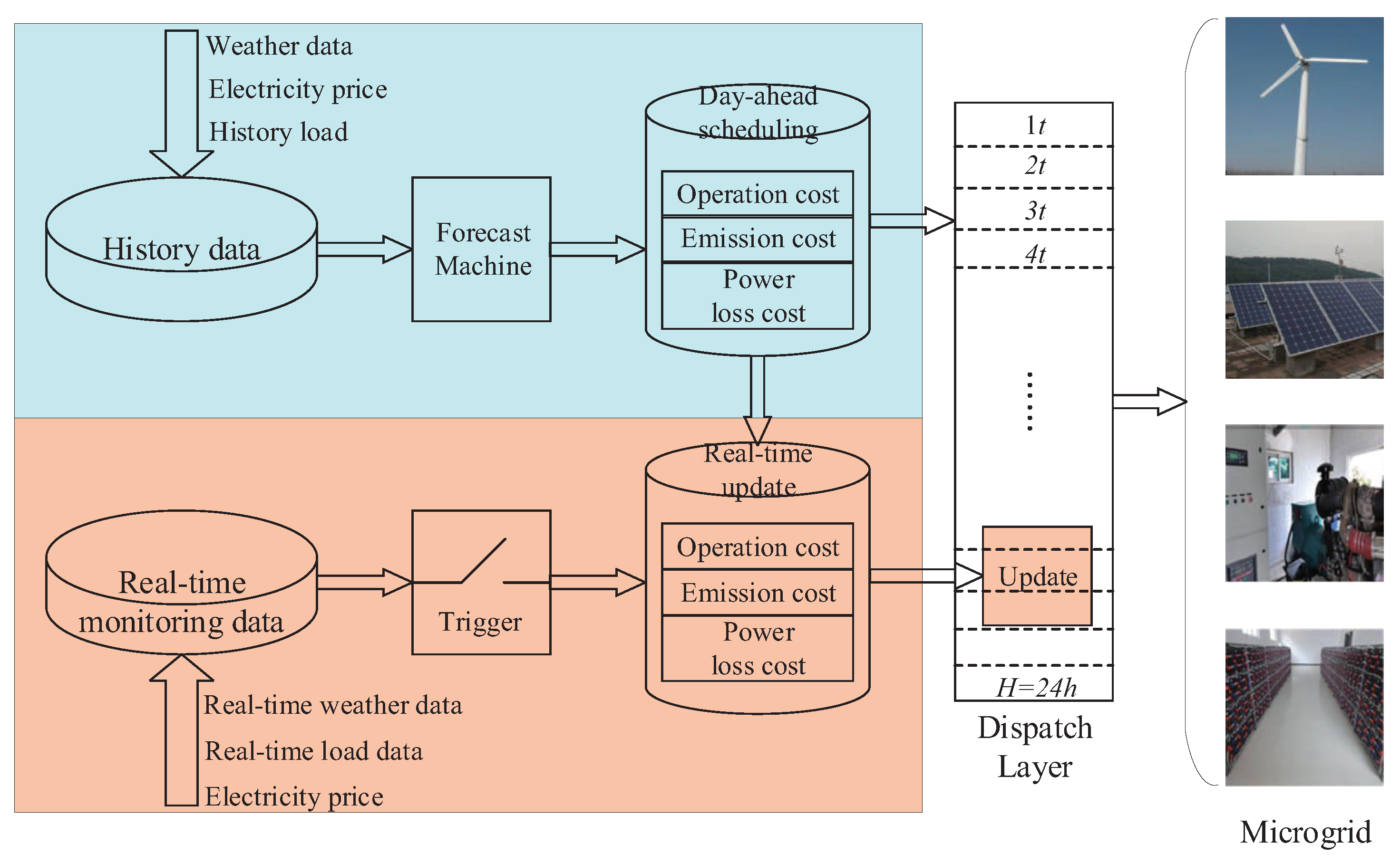
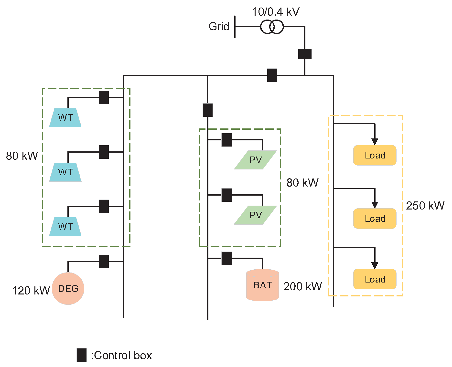
• A TSD model which consists of the day-ahead scheduling stage and the real-time update stage is proposed to optimize dispatch for microgrid energy management, as shown in Figure 1. The TSD model embodies different concepts, the first stage is the day-ahead scheduling based on forecast information to make dispatch plans for the next run day of a microgrid. The second stage, according to real-time information, updates the dispatch plan for the next few dispatch periods in the current running day.
• A novel hybrid PSO and opposition-based GSA (PSO-OGSA) is proposed to solve this complicated-constraints MOOD problem. Opposition-based learning (OL) is used to optimize the position distribution of initial populations in order to promote the search efficiency of GSA. The memory and community of PSO have been introduced to improve the acceleration mechanism of GSA, and the weight based inertial mass update rule has made the agents always move toward the best solution.

The rest of this paper is organized as follows. Section 2 contains the microgrid model and the optimization problem. Section 3 introduces the mathematical formulation of the proposed PSO-OGSA method to solve the optimization problem. Section 4 contains the simulation and results analysis. Finally, conclusions are summarized in Section 5.

2. Microgrid System and Problem Formulation

As shown in Figure 2, this microgrid consists of the wind turbines (WT), photovoltaic panel (PV), diesel generator (DEG), energy storage system (ESS) device, local load and controller and conversion devices, which can operate island or in grid-connected modes. The operators use both DGs and draw conventional energy from the main grid to meet load requirements, the surplus energy from the microgrid is stored in storage system for future use. In this paper, the operation cost, emission cost and power loss cost are considered as the multi-objectives to solve the MOOD problem.

2.1. Problem Formulation

The MOOD is a non-linear optimization problem that is subject to prevailing operation constraints and market decisions, and minimizes an objective function under constraints. The objective function can be formulated as follows:

$$min(f_1(x_t),f_2(x_t),\dots ,f_n(x_t))$$

(1)

$$\begin{array}{cc}\hfill s.t.& g(x_t)=0\hfill \\ & h(x_t)\le 0\hfill \end{array}$$

(2)

where $f_n(x_t)$ is the vector of n optimization objectives, $t\in H=\left\{\mathsf{\Delta }t,2\mathsf{\Delta }t,\dots ,T\right\}$ is the different dispatch period, $g(x_t)$ and $h(x_t)$ are the equality constraints and the inequality constraints, respectively, and $x_t$ is the set of decision variables, which includes the active/reactive power of all DGs, charge/discharge power of ESS and power loss of power conversion, and the local load. Therefore, x can be presented as:

$$x_t=\left\{P_{u,t},Q_{u,t},P_{g,t},P_{m,t},P_{ess,t}^c,P_{ess,t}^d,P_{loss,t},P_{load,t}\right\}$$

(3)

where ${\mathit{P}}_{\mathit{u},\mathit{t}}=({\mathit{P}}_{\mathit{wt}},{\mathit{P}}_{\mathit{pv}},{\mathit{P}}_{\mathit{deg}})$ and ${\mathit{Q}}_{\mathit{u},\mathit{t}}=({\mathit{Q}}_{\mathit{wt}},{\mathit{Q}}_{\mathit{pv}},{\mathit{Q}}_{\mathit{def}})$ are the active power and reactive power of WT, PV and DEG output in the microgrid, respectively, $P_{g,t}$ is the drawing active power from main grid, $P_{m,t}$ is the surplus energy of the microgrid selling to the main grid, $P_{ess,t}^c$ and $P_{ess,t}^d$ are the charge and discharge power of ESS, $P_{loss,t}$ is the loss power of energy transmission and conversion and $P_{load,t}$ is the load demand.

2.2. Objective Function

The MOOD adjusts the output power setpoints of DGs to meet the load demand; the operating cost, the emission cost of pollutants and the power loss cost of conversion devices are minimized simultaneously while satisfying constraints. The mathematical model of objective functions can be formulated as follows.

2.2.1. Operation Cost Function

During the running of the microgrid, the operation cost is equal to the sum of the electricity purchased from the main grid and the generation cost of WT, PV and DEG; the cost of ESS subtracts the profit of selling surplus energy to the main grid. Therefore, the operation cost function can be expressed by:

$$\begin{array}{cc}\hfill f_1(x_t)=\sum _{t=\mathsf{\Delta }t}^H& [C_b{P}_{g,t}{U}_{g,t}-C_s{P}_{m,t}{U}_{m,t}+C_{wt}\sum _{n=1}^{N_w}{P}_{wt,t}^n+C_{pv}\sum _{n=1}^{N_p}{P}_{pv,t}^n+\hfill \\ & C_{deg}\sum _{n=1}^{N_d}{P}_{deg,t}^n+C_{ess}(P_{ess,t}^c{U}_{bat,t}^c+P_{ess,t}^d{U}_{bat,t}^d)]\hfill \end{array}$$

(4)

where $C_b$ is the price of purchasing electricity from the main grid, $C_s$ is the price of selling surplus energy to the main grid, $U_{g,t}$ and $U_{m,t}$ are the state vector denoting the purchase or selling of electricity from the microgrid to the main grid, respectively, $C_{wt},C_{pv}$ and $C_{deg}$ are the unit generation cost of WT, PV and DEG, respectively, $C_{ess}$ is the cost coefficient of ESS and $N_w,N_p$ and $N_d$ are the generator numbers of WT, PV and DEG.

2.2.2. Emission Cost Function

The environment concerns from pollutant gases are considered as the second optimization objective. The emission cost function involves four of the most pollutant gases: CO${}_2$, SO${}_2$, NO and CO. The objective function can be express by:

$$\begin{array}{cc}\hfill f_2(x_t)& =\sum _{t=\mathsf{\Delta }t}^H\sum _{k=1}^4{C}_{env,k}{m}_k(x_t)\hfill \\ & =\sum _{t=\mathsf{\Delta }t}^H\sum _{k=1}^4{C}_{env,k}{u}_k(\sum _{n=1}^{N_d}{P}_{deg,t}^n+P_{g,t})\hfill \end{array}$$

(5)

where $m_k(x_t)$ is the mass of the emission pollutant gas k, $k=(1,2,3,4)$ represent four pollutant gases: CO${}_2$, SO${}_2$, NO and CO, $C_{env,k}$ is the cost coefficient of the pollutant gas k. The emissions of pollutants gas are calculated by the load efficiency and rate power of generator [9]; the emissions of pollutants gas can be formulated as follows:

$$m_k(x_t)=u_k{\alpha }_n{P}_{rate,k}{\tau }_k$$

(6)

where $u_k$ is the emissions per unit kWh of pollutant gas k in g/kWh, ${\alpha }_n$ is the load ratio of the generator n, $P_{rate}$ and $\tau$ are the rate power and the operation time of the generator n.

2.2.3. Power Loss Cost Function

The output power of DGs is not a standard product to supply the consumption terminal, and it is required to power conversion by the converter devices. The power electronic converter interface plays an important role in the sustainable energy production and use of microgrid. However, each conversion of converter has brought a litter power loss for DGs generation power. With the installed capacity of renewable sources increasing, in order to reduce the running cost of microgrid and improve the utilized efficiency of renewables, the power loss from a large amount of converts is an objective which must be taken into consideration for the MOOD problem.

The sum of transformer loss, conducting loss and switching loss of converters is considered as the power loss. The peak efficiency of a converter around 98% is found according to the loss analysis and efficiency measurement of the converter in [17]. To simplify the calculation of power loss, the 2% of conversion power is defined as the power loss of converter in this microgrid. The mathematical formulation of the power loss cost function can be described as follows:

$$\begin{array}{cc}\hfill f_3(x_t)& =\sum _{t=\mathsf{\Delta }t}^H{C}_{loss}{P}_{loss,t}(x_t)\hfill \\ & =\sum _{t=\mathsf{\Delta }t}^H{C}_{loss}{\sigma }_{loss}(\sum _{n=1}^{N_p}{P}_{pv,t}^n+\sum _{n=1}^{N_w}{P}_{wt,t}^n+\sum _{n=1}^{N_d}{P}_{deg,t}^n+P_{ess,t}^c+P_{ess,t}^d+P_{g,t}{U}_{g,t}+P_{m,t}{U}_{m,t})\hfill \end{array}$$

(7)

where $C_{loss}$ is the spot price of demand side in CNY/kWh, ${\sigma }_{loss}=0.02$ is the power loss coefficient of converters, $P_{loss,t}(x_t)$ is the power loss of all converters in the microgrid.

With the aforementioned objective functions, the goal of the MOOD problem can be expressed by:

$$min\left\{f_1(x_t),f_2(x_t),f_3(x_t)\right\}$$

(8)

The solution of Equation (8) achieves the minimization of the goal and finds the best optimal dispatch plan for microgrid running.

2.3. Constraints

Constraints indicate the restricted condition and the operation status of the microgrid when solving the MOOD problem. Constraint conditions are described as follows:

• Power balance:

  $$U_{g,t}{P}_{g,t}+P_{u,t}+P_{deg,t}+U_{bat,t}^d{P}_{ess,t}^d=U_{m,t}{P}_{m,t}+P_{load,t}+P_{loss,t}+U_{bat,t}^c{P}_{ess,t}^c$$

  (9)

  $$U_{g,t}+U_{m,t}\le 1,\left\{U_{g,t},U_{m,t}\right\}\in \left\{0,1\right\}$$

  (10)

  $$U_{bat,t}^c+U_{bat,t}^d\le 1,\left\{U_{bat,t}^c,U_{bat,t}^d\right\}\in \left\{0,1\right\}$$

  (11)
• Purchase electricity and sell power:

  $$\begin{array}{c}{P}_{g,t}^{min}\le P_{g,t}\le P_{g,t}^{max}\hfill \\ P_{m,t}^{min}\le P_{m,t}\le P_{m,t}^{max}\hfill \end{array}$$

  (12)
• Generator power:

  $$\begin{array}{c}0\le P_{wt}\le P_{wt}^{max}\hfill \\ 0\le P_{pv}\le P_{pv}^{max}\hfill \\ 0\le P_{deg}\le P_{deg}^{max}\hfill \end{array}$$

  (13)
• Battery limits:

  $$\begin{array}{c}0\le P_{bat}^c\le P_{bat}^{c,max}\hfill \\ 0\le P_{bat}^d\le P_{bat}^{d,max}\hfill \end{array}$$

  (14)
• Battery state of charge (SOC):

  $$SO{C}_{t+\mathsf{\Delta }t}=SO{C}_t+(P_{bat,t})\mathsf{\Delta }t/C_{bat}$$

  (15)

  $$SO{C}_{min}\le SO{C}_t\le SO{C}_{max}$$

  (16)

where Equation (9) presents the power balance constraint, Equation (10) ensures that the electricity is not allowed to be purchased and sold at the same moment, the charge and discharge of a battery are not allowed at same time according to Equation (11). $P_{g,t}^{min}$, $P_{g,t}^{max}$ and $P_{m,t}^{min}$, $P_{m,t}^{max}$ are the lower and upper boundaries of purchasing electricity from the main grid and surplus energy of the microgrid selling to the main grid, respectively, as indicated by Equation (12). $P_{wt}^{max},P_{pv}^{max}$ and $P_{deg}^{max}$ are maximum output power of wind turbine, photovoltaic and diesel generator, respectively. $P_{bat}^{c,max}$ and $P_{bat}^{d,max}$ are the maximum charge and discharge power by constraints in Equation (14). The $SO{C}_t$ is the state of charge at time interval t, $P_{bat,t}$ is the charging (or discharging) power at the time interval t, and $C_{bat}$ is the nominal capacity of the battery, as indicated by Equation (15). $SO{C}_{min}$ and $S0C_{max}$ are the minimum and maximum state of charge (SOC) of the battery by constraints in Equation (16).

3. Proposed Two-Stage Dispatch Model and Optimization Method

The day-ahead scheduling layer is based on forecast information (forecast generation power, electricity price, forecast load) to formulate a dispatch plan for power setpoints of generator units on the next day. Due to the forecast error, the real-time update stage is based on the real-time data (real-time output power, real-time load, electricity price) to update the dispatch plan for the next few dispatch periods. The objective functions of both stages are solved by the proposed PSO-OGSA under the constraints of the microgrid.

3.1. Two-Stage Dispatch Model

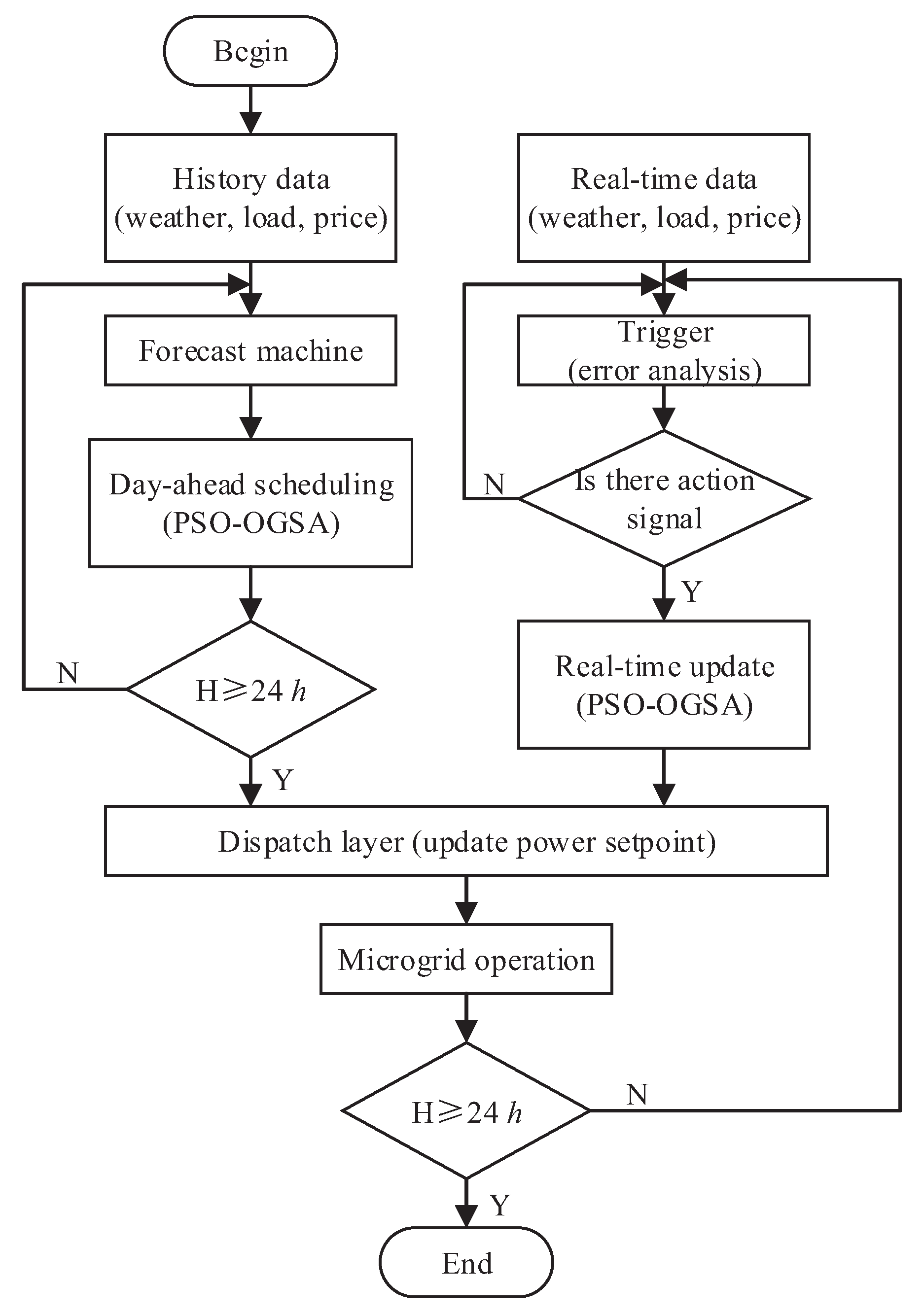
As shown in Figure 1, this model consists of two stages, the day-ahead scheduling stage and the real-time update stage. The dispatch time-step of the day-ahead scheduling stage and the real-time update stage are defined as 1 h and 15 min, respectively. A brief flow chart of the proposed TSD model to solve the MOOD problem is illustrated in Figure 3.

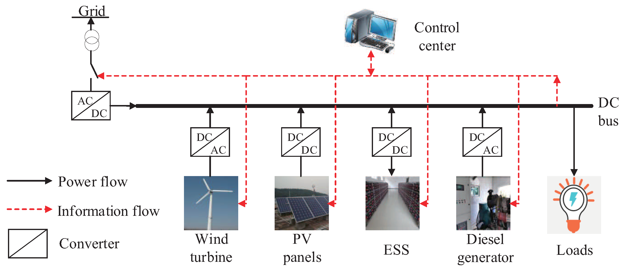
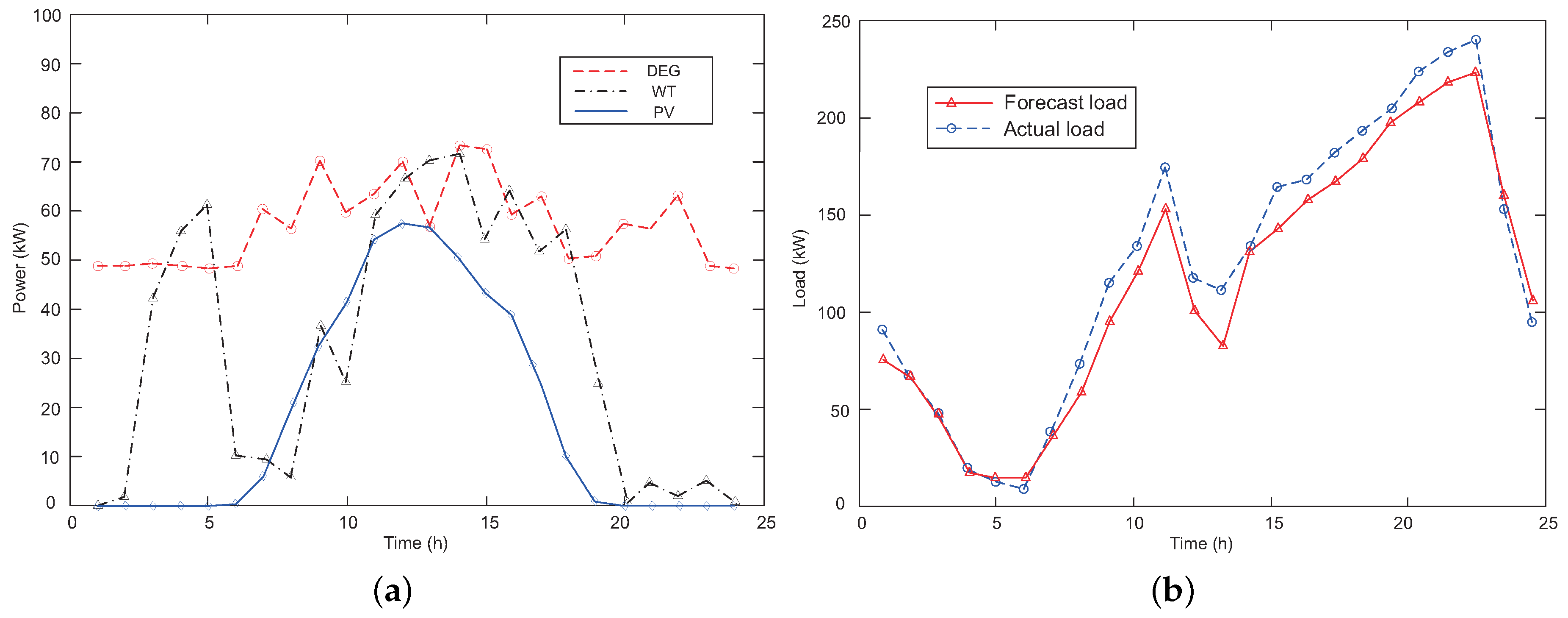
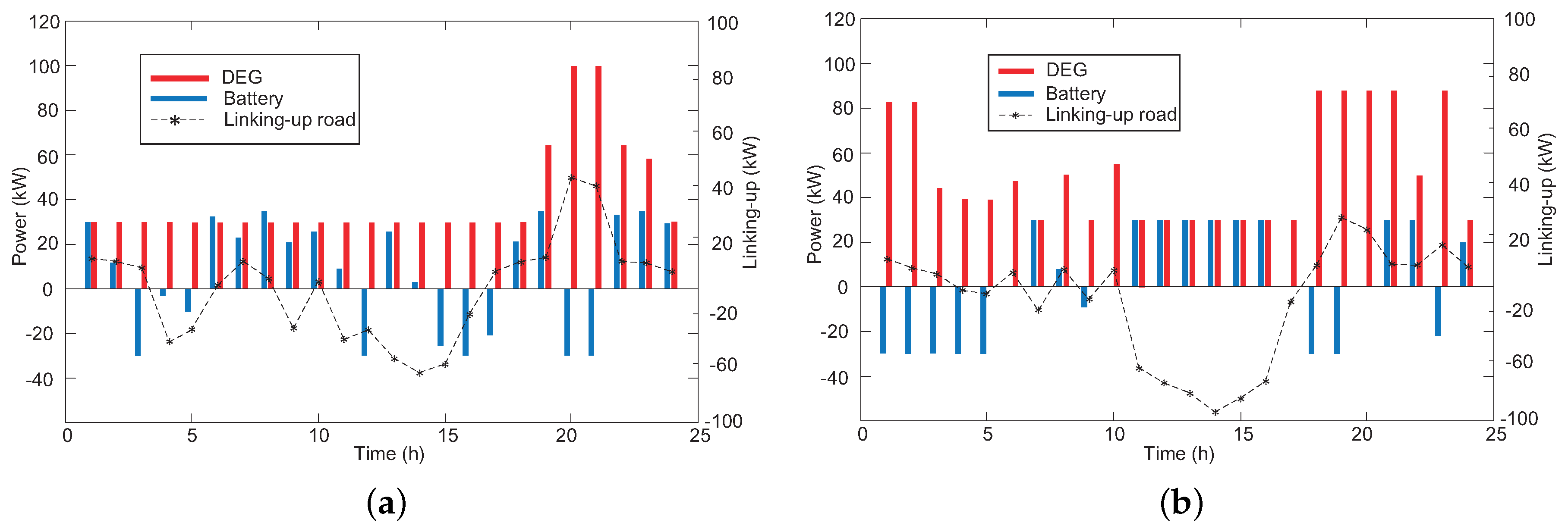
At the day-ahead scheduling stage, the dispatch plan is divided into 24 dispatch periods of 1 h and power setpoint is configured for generation units at each period. This stage is based on the forecast information from the forecast machine to formulate the dispatch plan. The day-ahead scheduling stage uses the proposed PSO-OGSA to optimize the operation cost function, emission cost function and power loss cost function according to the predicted power and load demand. The input data of the forecast machine mainly include weather information, electricity price and history load. Based on this information, the predicted power of generator units and load demand are obtained from the forecast machine for day-ahead scheduling at each period. Considering the forecast error, the predicted power and load demand fluctuate during the running of the microgrid. The fluctuation may leads to a mismatch between the actual load demand and the generation power in the dispatch periods. Therefore, the dispatch plan of the day-scheduling stage must update according to the real-time monitoring information.

The real-time update stage is described in 96 dispatch periods of 15 minutes, and recognizes the action signal of the trigger to formulate the dispatch plan for the next few dispatch periods. Based on the action signal of the trigger, the real-time update stage uses the proposed PSO-OGSA optimization objective functions to formulate and update the dispatch plan for the next few periods during the microgrid operation. The input data of the trigger are the real-time weather information, real-time generation power of generator units and real-time load demand from the microgrid. The action signal of the trigger is activated so that the error range is beyond the critical value, and the error is between the monitoring data and the forecast information. The trigger will export the new predicted power of generation units and load demand after sending the action signal. The real-time weather information mainly includes solar radiation, temperature, air pressure, wind speed, wind direction and humidity, which are obtained from the local meteorological department website. The critical value of the error range of generation power and load demand is set to 10%, and the critical value of the error range of meteorological information is set to 20%.

3.2. Proposed PSO-OGSA

3.2.1. Gravitational Search Algorithm

GSA is a heuristic optimization algorithm based on Newton’s law of gravity [27]. The solution of the optimization problem is considered as the agent of GSA consisting of different particles in the search space, and each agent attracts other agents through its own gravity force. The motion of agents obeys Newton’s law of motion to make the agent move toward the agent of the heaviest mass. The position of the heaviest mass corresponds to the optimum solution position of the optimization problem in the search space. The agent is specified by four parameters: Position, inertial mass, passive mass and gravity force.

Assume that a system with N agents, the position of the ith agent is described by:

$$X_i=(x_i^1,\dots ,x_i^d,\dots ,x_i^D)i=1,2,\dots ,N$$

(17)

where $x_i^d$ is the position of the ith agent in the dth dimension, D is the dimension of search space and N is the number of agents in the search space.

In the specific time t, the force acting on the agent i from the agent j is defined by:

$$F_{ij}^d(t)=G(t)\frac{M_{pi}(t)x{M}_{aj}(t)}{R_{ij}(t)+ϵ}(x_j^d(t)-x_i^d(t))$$

(18)

where $M_{pi}$ is the passive gravitational mass related to agent i, and $M_{aj}$ is the active gravitational mass related to agent j. $G(t)$ is the gravitational constant at time t and $ϵ$ is a small constant. $R_{ij}(t)$ is the Euclidean distance between the agent i and agent j by the following:

$$R_{ij}(t)=\left|\right|X_i(t)-X_j(t){\left|\right|}_2$$

(19)

The mass of the agents are calculated as follows:

$$m_i(t)=\frac{fi{t}_i(t)-worst(t)}{best(t)-worst(t)}$$

(20)

$$M_i(t)=\frac{m_i(t)}{{\displaystyle \sum _{j=1}^N}{m}_i(t)}$$

(21)

where $fi{t}_i(t)$ is the fitness value of agent i at time t and $M_i(t)$ is the mass of agents. For a minimization problem, $best(t)$ and $worst(t)$ are the best and worst fitness value of all agents at time t.

$$best(t)=\underset{j\in \left\{1,2,\dots ,N\right\}}{min}fi{t}_j(t)$$

(22)

$$worst(t)=\underset{j\in \left\{1,2,\dots ,N\right\}}{max}fi{t}_j(t)$$

(23)

To give a stochastic characteristic to the algorithm, suppose that the total force that acts on agent i in a dimension d be a randomly weighted sun of dth components of the forces exerted from other agents.

$$F_i^d(t)=\sum _{j\in Kbest,j\not\equiv i}ran{d}_j{F}_{ij}^d(t)$$

(24)

where $ran{d}_j$ is a random number between interval [0, 1]. $Kbest$ is a function of time, with the initial value $k_0$ at the beginning and decreasing with time. The acceleration of the agent i at time t is defined by:

$$a_i^d(t)=\frac{F_i^d(t)}{M_{ii}(t)}$$

(25)

where $M_{ii}(t)$ is the inertial mass of the agent i.

Calculating the gravitational constant $G(t)$ at time t uses the following:

$$G(t)=G_0{e}^{-\alpha \frac{t}{t_{max}}}$$

(26)

where $G_0$ is set to 100, $\alpha$ is set to 20 and t and $t_{max}$ are the current and the number of iterations, respectively.

The velocity and position of the agent i at next time $(t+1)$ could be calculated by employing the following:

$$v_i^d(t+1)=ran{d}_i{v}_i^d(t)+a_i^d(t)$$

(27)

$$x_i^d(t+1)=x_i^d(t)+v_i^d(t+1)$$

(28)

where $ran{d}_i$ is the random variable between interval [0, 1] and $v_i^d(t)$ and $x_i^d(t)$ are the velocity and the position of an agent in the d dimension at time t, respectively.

Repeating the above steps, the position of the heaviest mass is found out; the position corresponds to the position of the optimum solution of the optimization problem. The local search ability of GSA is weaker than the global search ability, and GSA is prone to optimal value oscillation.

3.2.2. Opposition-Based GSA

The initial solution of the GSA depends on the position of initial agents that randomly guess, and the distance between the initial solutions will effect the computation time of GSA. Moreover, the initial agent of random guesses may lead to the instability of the GSA searching efficiency. Therefore, on the initial stage of GSA, we change the relative position of the initial agents, and make agents closer to the optimal solution. The advantages of opposition-based learning are revolutionary jumps during the early learning stage, and the advantages are weakened gradually as learning continues [30]. Apparently, sudden switching to opposite values should only be utilized at the start to save time, and should not be maintained as the estimate is already in the vicinity of an existing solution.

Let $x\in [a,b]$ be a real number, the opposite number $\tilde{x}$ can be defined as:

$$\tilde{x}=a+b-x.$$

(29)

Assume $S=(x_1,\dots ,x_i,\dots ,x_N)$ is an original solution in d-dimension space with $x_1,\dots ,x_N\in R$ and $x_i\in [a_i,b_i](i=1,2,\dots ,N)$. Then, the related opposition point is defined as $({\tilde{x}}_1,\dots ,{\tilde{x}}_i,\dots ,{\tilde{x}}_N)$ where:

$${\tilde{x}}_i=a_i+b_i-x_i$$

(30)

Supposing a temporary space $[(x_1,{\tilde{x}}_1),\dots ,(x_i,{\tilde{x}}_i)\dots ,(x_N,{\tilde{x}}_N)]$ consists of the initial agent (solution) opposition value, and calculates the fitness of all agents. All agents $(x_i,{\tilde{x}}_i)$ from smallest to largest are sorted according to the fitness value of the agent. The N agents with the best fitness value are selected from the temporary space to form an initial population $P_0$.

In the initial population $P_0$, the elite strategy is used to generate new agents for 20% of the N solutions with the best fitness value, and add the new agents to the initial population $P_o$. The fitness value of 120% of the N solutions is calculated and sorted from smallest to largest, removing 20% of the N solutions with the worst fitness value. Finally, we can obtain the optimal initial population P. Among them, the new agents can be expressed as follows:

$$Q=R_{ij}(t)\times \frac{rand(-0.5,0.5)}{N}$$

(31)

$$x_{inew}(t)=x_i(t)\times Q$$

(32)

where Q is the transform factor of the new agent, $R_{ij}(t)$ represents the Euclidean distance between the solution and the adjoining solution and N is the number of the initial population.

3.2.3. Particle Swarm Optimization Based OGSA

GSA must use the exploration to avoid trapping a local optimum at the beginning for the optimization problem [27]. As similar with the PSO, the solutions of GSA are obtained by the agents moving toward the global optimal solution in the search space. In the GSA, the motion direction of agents is attracted by the total force from other agents. However, when the position of the agents is updated, only considering the current position of the agent, the memory information of the agent is not yet taken into account.

Compared with the GSA, the position of the PSO particles is determined by both the current position information and the community information of particles. Therefore, the performance of the memory and community exchanges of PSO are introduced to improve the search ability of GSA. The motion direction of agents is decided by the new path on GSA, and the new path obeys both Newton’s law of motion and additional performance of the memory and community of PSO. The velocity and position of agents in the PSO-OGSA can be formulated as follows:

$$\begin{array}{cc}\hfill v_i^d(t+1)=& c_3(ran{d}_i{v}_i^d(t)+a_i^d)+\hfill \\ & (1-c_3)[c_{1}ran{d}_1(p_{best}^d-x_i^d(t))+c_{2}ran{d}_2(g_{best}^d-x_i^d(t))]\hfill \end{array}$$

(33)

$$x_i^d(t+1)=x_i^d(t)+v_i^d(t+1)$$

(34)

where $c_1$ and $c_2$ are two constants between the interval [0, 1], $ran{d}_i$, $ran{d}_1$, and $ran{d}_2$ are the random variables between the interval [0, 1], $c_3$ is a variable within [0, 1] to determine stochastic impacts of GSA acceleration and PSO velocity on PSO-OGSA, $p_{best}^d$ is the historical optimal value of the agent i and $g_{best}^d$ is the global optimal value of all agents.

The process of the proposed PSO-OGSA can be summarized as in

Table 1. Flowchart of PSO-OGSA.

Step 1: Opposition-based for initial population.

Generate uniformly distributed initial population $P_{0_{i,j}}$

Opposition population $O{P}_{0_{i,j}}=a_j+b_j-P_{0_{i,j}}$

$i\le N$: population size. $j\le D$: problem dimension

Step 2: Select the N fittest agents from set of $\left\{P_0,O{P}_0\right\}$ as initial population $P_0$

Step 3: Select 20% of the N fittest agents to generate new agents according to Equation(31) and Equation(32)

add 20% of the N new agents into the $P_{0_{i,j}}$ and calculate fitness

remove 20% of the N worst fitness agents

End of opposition-based learning

Step 4: Fitness evaluation of agents according to Equation(22) and Equation(23)

Step 5: Calculate $G(t)$, $M_i(t)$

Step 6: Update the mass $M_{inew}$ of agents according to Equation(35) and Equation(36)

Step 7: Total force $F_i^d(t)$, acceleration $a_i^d(t)$

Step 8: Update the velocity $v_i^d(t)$ and position $x_i^d(t)$ according to Equation(33) and Equation(34)

Step 9: PSO based generation jumping

calculate the fitness of all agents $fi{t}_j(t)$

calculate $p_{best}^d$, $g_{best}^d$

Step 10: Repeat steps 4–10 until the stopping criteria is met.

; the global optimal solution has been observed by each agent and moves toward it so that the movement process always obeys the law of motion. The total force of the heaviest agent is greater than the force of other agents; in other words, the solution represented by the heaviest agent is better than the solution represented by the light agent. In order to make the gravity force of the heavier agent stronger and the gravity force of light agent weaker, the heavier agent can move quickly toward the global optimal solution in the search space. A weight proposed is used to update the mass of all agents at the iteration time, and it not only speeds up the agent movement to the global optimal solution, but also improves the convergence of PSO-OGSA. The weight H is calculated according to the mass of the agent at each iteration, and weight H can be defined by the following:

$$\begin{array}{c}\hfill H_i(t)=\frac{C_{min}{M}_{min}-C_{max}{M}_{max}}{M_{min}-M_{max}}-M_i(t)\end{array}$$

(35)

$$M_{inew}=H_i(t)\times M_i(t)$$

(36)

where $H_i(t)$ represents the weight of the agent i, $C_{min}$ = 1 and $C_{max}$ = 5 are the minimum and maximum of the weight, respectively, and $M_{max}$ and $M_{min}$ are the maximum and minimum of the mass agent in the search space, respectively.

4. Results and Discussion

In this section, an actual microgrid system is used to verify the effects and validations of the two-stage dispatch model and the proposed PSO-OGSA method. Five canonical benchmark test functions are used to validate the performance of the proposed PSO-OGSA. All the simulations are implemented in Matlab 2014b on a PC with 3.2 GHz CPU and 4G RAM.

4.1. Validate the PSO-OGSA Method

In order to analyze the performance of the PSO-OGSA, we have used five canonical benchmark test functions to evaluate the PSO-OGSA with other algorithms. The five canonical benchmark test functions are minimum problems as shown in

Table 2. Benchmark test functions for validation [27].

Function Name	Function Expression	Domain	Trait
$f_{Ros}$, Rosenbrock	$f_1(x)={\displaystyle \sum _{i=1}^{n-1}}(100{(x_{i+1}-x_i^2)}^2+{(x_i-1)}^2)$	[−30,30]	Unimodal
$f_{Sch}$, Schwefel	$f_2(x)={\displaystyle \sum _{i=1}^n}-x_{i}sin(\sqrt{|}{x}_i|)$	[−500,500]	Multimodal
$f_{Ras}$, Rastrigin	$f_3(x)={\displaystyle \sum _{i=1}^n}(x_i^2-10cos(2\pi x_i)+10)$	[−5.12,5.12]	Multimodal
$f_{Gri}$, Griewank	$f_4(x)={\displaystyle \sum _{i=1}^n}\frac{x_i^2}{4000}-{\prod }_{i=1}^n(cos(\frac{x_i}{\sqrt{i}}))+1$	[−600,600]	Multimodal
$f_{Ack}$, Ackley	$f_5(x)=-20exp(-0.2\sqrt{\frac{}{}}1n{\displaystyle \sum _{i=1}^n}{x}_i^2)-exp(\frac{1}{n}{\displaystyle \sum _{i=1}^n}cos(2\pi x_i))+20+e$	[−30,30]	Mulyimodal

; n is the dimension of test functions [31]. The Rosenbrock test function is a simple unimodal function, and it has a single local optimum and global optimum. The other test functions are multimodal functions with many local optima, and the complexity of test functions and the amount of local optima have increased with increasing dimension. Therefore, these test functions with different features are used to testify to the effectiveness of the PSO-OGSA method.

In the validation experiment, the benchmark test functions have 30 trails for each algorithm, and the stop criteria of each run is to reach the maximum iteration. The maximum iteration is set to 1000. For the parameter settings of algorithms, we have configured as recommended according to the related literature [27,32]. For instance, the initial value of $k_0$ of GSA is set to the total number of agents and its final value decreases linearly to 2% of its initial value. $G_0$ is set to 100, and $\alpha$ is fixed at 20.

Two different dimension sizes $D=10$ and $D=30$ are tested for the canonical benchmark test functions by the proposed PSO-OGSA method. According to the discussion in the Section 3, the parameter settings of PSO-OGSA are set for this simulation experiment: $N=50$, $c_1=0.5$ and $c_2=1.5$. For the parameters of PSO, we use these settings: Population sizes $N=50,c_1=2.0,c_2=2.0$ and wight $\omega$ is deceased linearly from 0.9 to 0.2. Comparing the proposed PSO-GSA with the PSO and GSA approaches, the mean best fitness $Ave$ and the best fitness $Best$ of these methods for each test function is recorded in

Table 3. The mean best fitness of different methods for five benchmark test functions.

Function	Dimension (D)	PSO		GSA		PSO-OGSA
		$\mathit{Ave}$	$\mathit{Best}$	$\mathit{Ave}$	$\mathit{Best}$	$\mathit{Ave}$	$\mathit{Best}$
$f_{Ros}$	10	2.01E+02	15.59E+00	4.30E+00	3.82E+00	2.98E−03	2.06E−03
	30	3.71E+01	1.97E+01	2.83E+01	2.50E+01	4.20E−03	3.89E−05
$f_{Sch}$	10	−1.14E+01	−1.20E+01	−3.05E+01	−1.55E+03	−2.94E+03	−3.47E+03
	30	−3.54E+01	−3.54E+01	−4.91E+00	−3.16E+03	−7.97E+03	−9.54E+03
$f_{Ras}$	10	1.99E+01	4.97E+00	2.95E+00	2.98E+00	1.17E−06	1.31E−07
	30	1.18E+02	5.17E+01	1.43E+01	1.49E+01	4.25E−06	5.57E−05
$f_{Gri}$	10	2.94E−08	1.87E−09	2.74E+02	9.04E+02	2.98E−10	3.79E−11
	30	3.18E−07	2.41E−08	8.77E+02	6.04E+02	7.80E−11	3.65E−12
$f_{Ack}$	10	4.20E−03	9.38E−04	5.73E−04	1.08E−04	4.81E−10	2.66E−11
	30	3.30E−03	9.46E−04	2.60E−04	1.73E−04	1.30E−09	8.13E−10

$Ave$: Indicates average of best function values in 30 runs. $Best$: Indicates the best result in 30 runs.

. The results are average over 30 runs and the best results are indicated in bold type. From the results, it can be seen that the performance of the proposed PSO-OGSA is better than the other two methods. The optimization performance of the proposed PSO-OGSA is more powerful with the dimension of test function increasing.

To verify the convergence rate of the proposed PSO-OGSA, compare the PSO with GSA to show the performance of PSO-OGSA. The dimension of these functions is set to 30, and the results are the averaged best-so-far solution as shown in Figure 4. For the Rosenbrock function, the convergence rate of the search approach is more important than the final results, as the Rosenbrock function is a unidoal function. As shown in Figure 4a, the convergence rate of the PSO-OGSA is better than the other two approaches: PSO and GSA. For the multimodal functions, they are very difficult to optimize due to them having many local optimums. So, obtaining the best final results is important. As shown in Figure 4b–d, the proposed PSO-OGSA compared with the other two approaches has the best final optimum, and reflects the performance of PSO-OGSA escape from the localization trap quickly. According to Figure 4, we can conclude that the amount of the local optimum increases exponentially as the dimension of the function increases.

The convergence rate of benchmark test functions are verified by the PSO-OGSA, PSO and GSA in these figures, and shows that the proposed PSO-OGSA performs better than the standard PSO and GSA in terms of convergence rate.

4.2. A Microgrid Test System

In this section, the microgrid structure consisting of wind-photovoltaic-battery-diesel generator is shown in Figure 5. The renewable generation units, storage system, diesel generator and load are connected with DC bus; each generation unit is connected with the bidirectional converter, and this microgrid system is connected with the power grid. The conversion efficiency of photovoltaic array is considered as $18.5\%$. The cut-in speed 3 m/s, cut-out speed 35 m/s and cut-rate speed 10 m/s are for each wind turbine. The self discharge efficiency of battery is 10%. In the following simulations, the wind turbines and photovoltaic arrays generation cost are set to 0.6 CNY/kWh and 1.2 CNY/kWh, respectively. According to the above discussion, the parameters set for the PSO-OGSA are set for this simulation: N = 50, $c_1=0.5,c_2$ = 1.5, $G_0$ = 100, $\alpha$ = 20, and maximum iteration number is set to 1000.

The parameters of each generator unit in this microgrid are shown in

Table 4. Numerical data of distributed generations in the microgrid system.

Unit	Max Power (kW)	Min Power (kW)
Wind turbine	80	0
Photovoltaic cell	80	0
Battery	200	−100
Diesel generator	120	30

, and the emission cost and emission coefficient [33] of different pollutants are shown in

Table 5. Emission cost and emission coefficient of different pollutants.

Type	Externality Cost (CNY/kg)	Emission Factors for DEG (g/kWh)
NO${}_x$	26.52	0.6188
SO${}_2$	6.33	0.4641
CO${}_2$	0.089	232.0373
CO	0.1406	2.320

. The WT predicted power, PV predicted power and DEG predicted power are shown in Figure 6a, and the actual load fluctuation of the microgrid operation is shown in Figure 6b. Due to the fluctuation of output power from the renewable sources, the DEG is configured to follow the microgrid operation, and prioritize utilizing the output power of DEG.

In order to verify the effectiveness of the proposed TSD model in the actual microgrid operation, evaluating the performance of the real-time scheduling randomly adjusts the load demand of the microgrid at a certain period on the current running day, as shown in Figure 6b. The operation cost, emission cost and power loss cost are considered as the optimization objectives for the proposed PSO-OGSA. As shown in Figure 7a, the operation cost of the microgrid is the minimum; the difference of load demand is shared by the storage batteries and the diesel generator. The storage batteries charge at the low electricity price period and discharge at the high electricity price period; the other period is determined by the operation cost of the storage batteries and the diesel generator. When the emission cost is minimum, as shown in Figure 7b, the difference of load demand is supplied by the storage batteries, the output power of DEG is in the minimum generated power.

Performance of the proposed PSO-OGSA has been validated on the five benchmark functions, and the convergence rate of the PSO-OGSA is superior to the other two methods.To evaluate the performance of the proposed PSO-OGSA for finding the optimal solution of the MOOD problem. The PSO-OGSA, PSO and basic GSA are used to solve the MOOD problem for this microgrid. The algorithm parameter settings, computer configurations and programming software in this section are the same as those of Section 4.1. For all simulation experiments, the population size is set to 50, and the maximum iteration number is set to 1000.

The comparative convergence of the best solutions of three different methods for the operation cost, emission cost, power loss cost and total cost are shown in Figure 8. From these figures, it is shown clearly that the proposed PSO-OGSA converges smoothly to the optimum value in the optimization process. The proposed PSO-OGSA algorithm outperforms the PSO and GSA methods as a whole; it has the advantage of reducing emission cost and loss cost. The target values of multi-objective optimization of different methods are compared in

Table 6. Comparison of the detail data for the test microgrid.

Methods	Operation Cost (CNY)	Emission Cost (CNY)	Power Loss Cost (CNY)	Total Cost (CNY)	Simulation Time (s)
PSO	319.17	42.51	20.18	384.63	38.1
GSA	321.94	41.93	21.07	382.17	44.7
PSO-OGSA	304.91	36.27	19.25	360.43	43.9

, and it appears that the proposed algorithm has the best performance when comparing other population-based optimization algorithm.

5. Conclusions

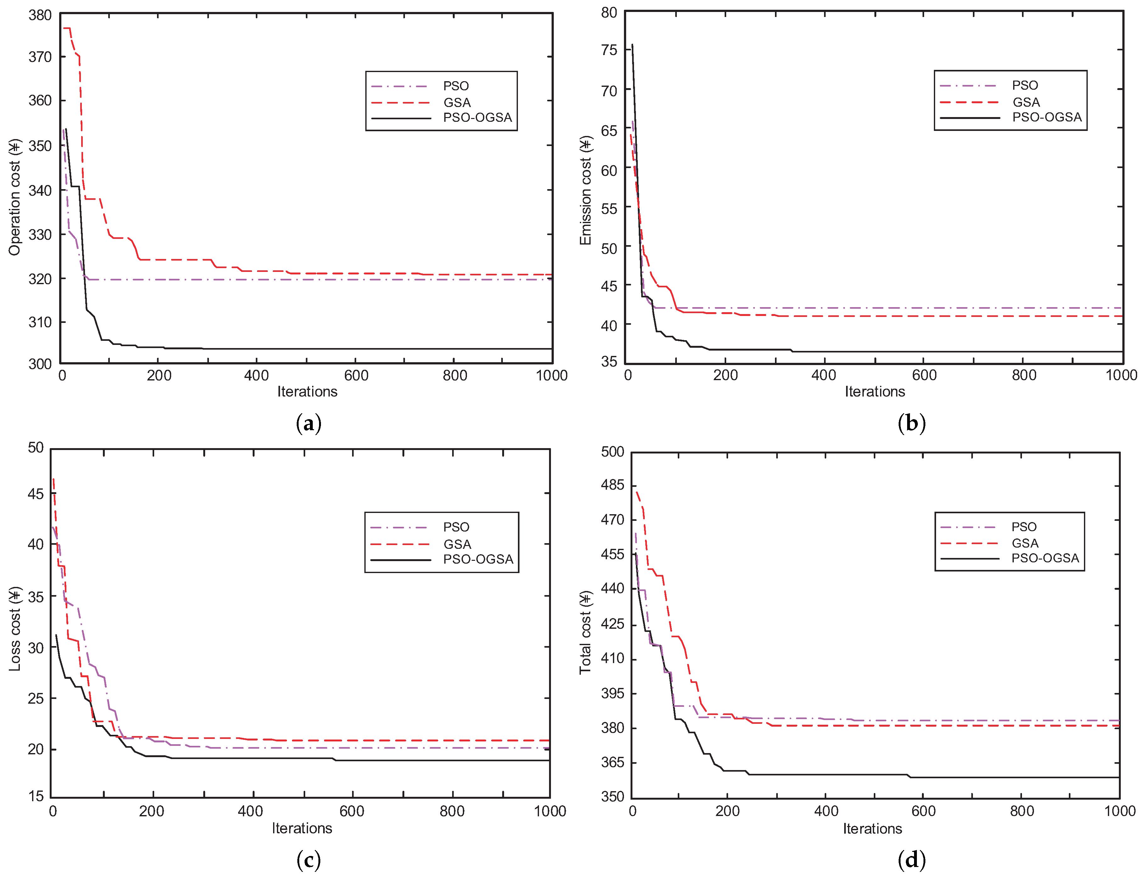
A TSD dispatch model combined the day-ahead scheduling and the real-time scheduling was proposed to apply optimization dispatch in order to minimize the total cost of microgrid operation. In this paper, we considered the power loss of the converters, and combined the operation cost with the emission cost to formulate the multi-objective optimization model. We proposed a hybrid particle swarm optimization and opposition-based learning gravity search algorithm to find the best solution of the dispatch plan for MOOD problem in the test microgrid. Based on the production forecast of WT and PV and load demand, the SOC of the storage batteries and the generation power of the diesel generator, the TSD model is used to search the optimal path by all possible system states in the 24-h dispatch planning. If the difference between day-ahead forecast and 15 min forecast of the current running is greater than the 10% power reserve, the dispatch plans are updated to recalculate the power setpoint for each generation unit. This PSO-OGSA algorithm enables us to find the optimization dispatch values while satisfying the constraint conditions.

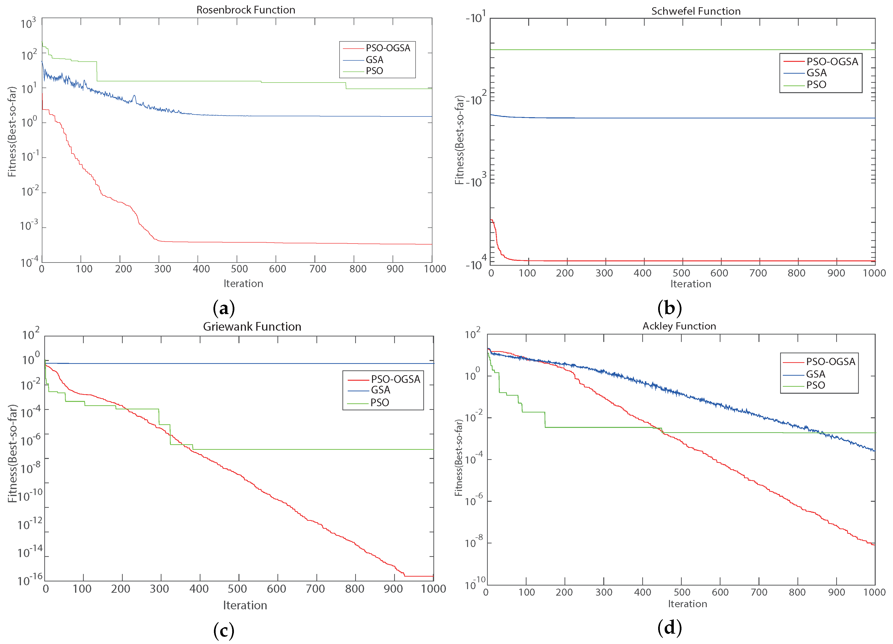
For the PSO-OGSA, opposition-based learning is used to optimize the initial population agents for GSA and strengthen the capacity of escaping from the localization trap quickly. The memory and community of PSO are introduced to improve the acceleration mechanism of GSA, and add a weight-based inertial mass update rule to make the agents speed up toward the best solution. The PSO-OGSA has been tested on five benchmark functions to validate the effectiveness, and the TSD model has been implemented into an actual microgrid system to simulate in real-time dispatch. The optimal results of PSO-OGSA are compared with the results from other algorithms, and demonstrate that the proposed approach is effective to solve the MOOD problem for a microgrid.

References

1. Zeng, J.; Wang, Q.; Liu, J.; Chen, J.; Chen, H. A Potential Game Approach to Distributed Operational Optimization for Microgrid Energy Management With Renewable Energy and Demand Response. IEEE Trans. Ind. Electron. 2019, 66, 4479–4489. [Google Scholar] [CrossRef]
2. Shuai, H.; Fang, J.; Ai, X.; Tang, Y.; Wen, J.; He, H. Stochastic optimization of economic dispatch for microgrid based on approximate dynamic programming. IEEE Trans. Smart Grid 2018, 10, 2440–2452. [Google Scholar] [CrossRef]
3. Mengelkamp, E.; Gärttner, J.; Rock, K.; Kessler, S.; Orsini, L.; Weinhardt, C. Designing microgrid energy markets: A case study: The Brooklyn Microgrid. Appl. Energy 2018, 210, 870–880. [Google Scholar] [CrossRef]
4. Sandgani, M.R.; Sirouspour, S. Priority-based microgrid energy management in a network environment. IEEE Trans. Sustain. Energy 2018, 9, 980–990. [Google Scholar] [CrossRef]
5. Carpinelli, G.; Mottola, F.; Proto, D.; Russo, A. A multi-objective approach for microgrid scheduling. IEEE Trans. Smart Grid 2016, 8, 2109–2118. [Google Scholar] [CrossRef]
6. Amicarelli, E.; Tran, T.Q.; Bacha, S. Optimization algorithm for microgrids day-ahead scheduling and aggregator proposal. In Proceedings of the 2017 IEEE International Conference on Environment and Electrical Engineering and 2017 IEEE Industrial and Commercial Power Systems Europe (EEEIC/I&CPS Europe), Milan, Italy, 6–9 June 2017. [Google Scholar]
7. Chybowski, L.; Gawdzińska, K. On the Possibilities of Applying the AHP Method to a Multi-criteria Component Importance Analysis of Complex Technical Objects. Adv. Intell. Syst. Comput. 2016, 701–710. [Google Scholar]
8. Shamsi, P.; Xie, H.; Longe, A.; Joo, J.Y. Economic dispatch for an agent-based community microgrid. IEEE Trans. Smart Grid 2015, 7, 2317–2324. [Google Scholar] [CrossRef]
9. Kanchev, H.; Colas, F.; Lazarov, V.; Francois, B. Emission reduction and economical optimization of an urban microgrid operation including dispatched pv-based active generators. IEEE Trans. Sustain. Energy 2014, 5, 1397–1405. [Google Scholar] [CrossRef]
10. Chiang, C.-L.; Chai, C.-W. A Multi-Objective Optimization for Power Economic Dispatch. In Proceedings of the 2006 IEEE International Conference on Systems, Man and Cybernetics, Taipei, Tiwan, 8–11 October 2006. [Google Scholar]
11. Sarfi, V.; Niazazari, I.; Livani, H. Multiobjective fireworks optimization framework for economic emission dispatch in microgrids. In Proceedings of the 2016 IEEE North American Power Symposium, Charlotte, NC, USA, 4–6 October 2016. [Google Scholar]
12. Zhang, Y.; Gatsis, N.; Giannakis, G.B. Robust energy management for microgrids with high-penetration renewables. IEEE Trans. Sustain. Energy 2013, 4, 944–953. [Google Scholar] [CrossRef]
13. Cardoso Bora, T.; Cocco Mariani, V.; dos Santos Coelho, L. Multi-objective optimization of the environmental-economic dispatch with reinforcement learning based on non-dominated sorting genetic algorithm. Appl. Therm. Eng. 2018, 146, 688–700. [Google Scholar] [CrossRef]
14. Xu, X.; Hu, Z.; Su, Q.; Xiong, Z. Multiobjective Collective Decision Optimization Algorithm for Economic Emission Dispatch Problem. Complexity 2018, 2018, 1027193. [Google Scholar] [CrossRef]
15. Hsieh, Y.P.; Chen, J.F.; Yang, L.S.; Wu, C.Y.; Liu, W.S. High-conversion-ratio bidirectional dc–dc converter with coupled inductor. IEEE Trans. Ind. Electron. 2014, 61, 210–222. [Google Scholar] [CrossRef]
16. Kim, H.S.; Ryu, M.H.; Baek, J.W.; Jung, J.H. High-Efficiency Isolated Bidirectional AC–DC Converter for a DC Distribution System. IEEE Trans. Power Electron. 2013, 28, 1642–1654. [Google Scholar] [CrossRef]
17. Zhang, J.H.; Kim, R.Y.; Lai, J.S. High-power density design of a soft-switching high-power bidirectional dc–dc converter. IEEE Trans. Power Electron. 2007, 22, 1145–1153. [Google Scholar] [CrossRef]
18. An, L.N.; Quoc-Tuan, T. Optimal energy management for grid connected microgrid by using dynamic programming method. In Proceedings of the 2015 IEEE Power & Energy Society General Meeting, Denver, CO, USA, 26–30 July 2015; pp. 1–5. [Google Scholar]
19. Wu, X.; Hu, X.; Moura, S.; Yin, X.; Pickert, V. Stochastic control of smart home energy management with plug-in electric vehicle battery energy storage and photovoltaic array. J. Power Sources 2016, 333, 203–212. [Google Scholar] [CrossRef] [Green Version]
20. Dehghanpour, K.; Nehrir, H. Real-time multiobjective microgrid power management using distributed optimization in an agent-based bargaining framework. IEEE Trans. Smart Grid 2018, 9, 6318–6327. [Google Scholar] [CrossRef]
21. Wouters, C.; Fraga, E.S.; James, A.M. An energy integrated, multi-microgrid, MILP (mixed-integer linear programming) approach for residential distributed energy system planning–a South Australian case-study. Energy 2015, 85, 30–44. [Google Scholar] [CrossRef]
22. Hong, Y.Y.; Hsiao, M.C.; Chang, Y.R.; Lee, Y.D.; Huang, H.C. Multiscenario underfrequency load shedding in a microgrid consisting of intermittent renewables. IEEE Trans. Power Deliv. 2013, 28, 1610–1617. [Google Scholar] [CrossRef]
23. Liao, G.C. Solve environmental economic dispatch of Smart MicroGrid containing distributed generation system—Using chaotic quantum genetic algorithm. Int. J. Elect. Power Energy Syst. 2012, 43, 779–787. [Google Scholar] [CrossRef]
24. Li, P.; Xu, D.; Zhou, Z.; Lee, W.J.; Zhao, B. Stochastic optimal operation of microgrid based on chaotic binary particle swarm optimization. IEEE Trans. Smart Grid 2016, 7, 66–73. [Google Scholar] [CrossRef]
25. Radosavljević, J.; Jevtić, M.; Klimenta, D. Energy and operation management of a microgrid using particle swarm optimization. Eng. Optim. 2016, 48, 811–830. [Google Scholar] [CrossRef]
26. Yuan, X.; Zhang, B.; Wang, P.; Liang, J.; Yuan, Y.; Huang, Y.; Lei, X. Multi-objective optimal power flow based on improved strength Pareto evolutionary algorithm. Energy 2017, 122, 70–82. [Google Scholar] [CrossRef]
27. Rashedi, E.; Nezamabadi-Pour, H.; Saryazdi, S. GSA: A gravitational search algorithm. Inf. Sci. 2009, 179, 2232–2248. [Google Scholar] [CrossRef]
28. Duman, S.; Guvenc, U.; Sonmez, Y.; Yörükeren, N. Optimal power flow using gravitational search algorithm. Energy Convers. Manag. 2012, 59, 86–95. [Google Scholar] [CrossRef]
29. Li, C.S.; Zhou, J.Z. Parameters identification of hydraulic turbine governing system using improved gravitational search algorithm. Energy Convers. Manag. 2011, 52, 374–381. [Google Scholar] [CrossRef]
30. Tizhoosh, H.R. Opposition-Based Learning: A New Scheme for Machine Intelligence. In Proceedings of the 2006 International Conference on Computational Intelligence for Modelling, Control and Automation and International Conference on Intelligent Agents, Web Technologies and Internet Commerce (CIMCA- IAWTIC’05), Vienna, Austria, 28–30 November 2005; pp. 695–701. [Google Scholar]
31. Jiang, S.; Ji, Z.; Shen, Y. A novel hybrid parti cle swarm optimization and gravitational search algorithm for solving economic emission load dispatch problems with various practical constraints. Int. J. Elect. Power Energy Syst. 2014, 55, 628–644. [Google Scholar] [CrossRef]
32. Zhang, Y.; Gong, D.W.; Ding, Z. A bare-bones multi-objective particle swarm optimization algorithm for environmental/economic dispatch. Inf. Sci. 2012, 192, 213–227. [Google Scholar] [CrossRef]
33. Mohamed, F.A.; Koivo, H.N. System modelling and online optimal management of microgrid using mesh adaptive direct search. Int. J. Elect. Power Energy Syst. 2010, 32, 398–407. [Google Scholar] [CrossRef]
Figure 1. The block diagram of two-stage dispatch (TSD) for a microgrid.
Energies 12 02160 g001
Figure 2. The schematic diagram of microgrid system.
Energies 12 02160 g002
Figure 3. Simple flow chart of the proposed TSD model for a MOOD problem.
Energies 12 02160 g003
Figure 4. Comparative convergence behaviors of the PSO-OGSA, PSO and GSA for some benchmark test functions, (a) the Rosenbrock function, (b) the Schwefel function, (c) the Griewank function, and (d) the Ackley function.
Energies 12 02160 g004
Figure 5. The transmission network of the test microgrid system.
Energies 12 02160 g005
Figure 6. The predicted power of the distributed system and load demand in the microgrid. (a) Prediction power. (b) Load demand.
Energies 12 02160 g006
Figure 7. Output power of the storage batteries and the diesel generator in the microgrid; (a) the operation cost minimum, (b) the emission cost minimum.
Energies 12 02160 g007
Figure 8. Comparative convergence for the GSA, PSO and PSO-OGSA for test microgrid. (a) Operation cost. (b) Emission cost. (c) Loss cost. (d) Total cost.
Energies 12 02160 g008